Exercise 1 (Gibbs Sampler for Marketing Mix Model) A simple MMM without regressors assumes that sales \(Y_t\) follow a dynamic process influenced only by latent factors like baseline sales and carryover effects. A basic state-space representation could be: \[
\begin{aligned}
y_t \sim &N(\mu,\tau^{-1})\\
\mu \sim & N(0,1)\\
\tau \sim & Gamma(2,1).
\end{aligned}
\]
Here \(\mu\) is the baseline sales level (unknown and measured on normalized scale), and \(\tau\) is the precision of the sales data. The goal is to implement a Gibbs sample for the posterior \(\mu,\tau | y\), where \(y = (y_1,\ldots,y_n)\) is the observed data. Gibbs sampler algorithms iterates between two steps:
Sample \(\mu_i\) from \(\mu \mid \tau_{i-1}, y\)
Sample \(\tau_i\) from \(\tau_i \mid \mu_i, y\)
Show that those full conditional distributions are given by \[
\begin{aligned}
\mu \mid \tau, y \sim & N\left(\dfrac{\tau n\bar y}{1+n\tau},\dfrac{1}{1+n\tau}\right)\\
\tau \mid \mu,y \sim & \mathrm{Gamma}\left(2+\dfrac{n}{2}, 1+\dfrac{1}{2}\sum_{i=1}^{n}(y_i-\mu)^2\right)
\end{aligned}
\]
Use formulas for full conditional distributions and implement the Gibbs sampler. The data \(y\) is in the file MCMCexampleData.txt.
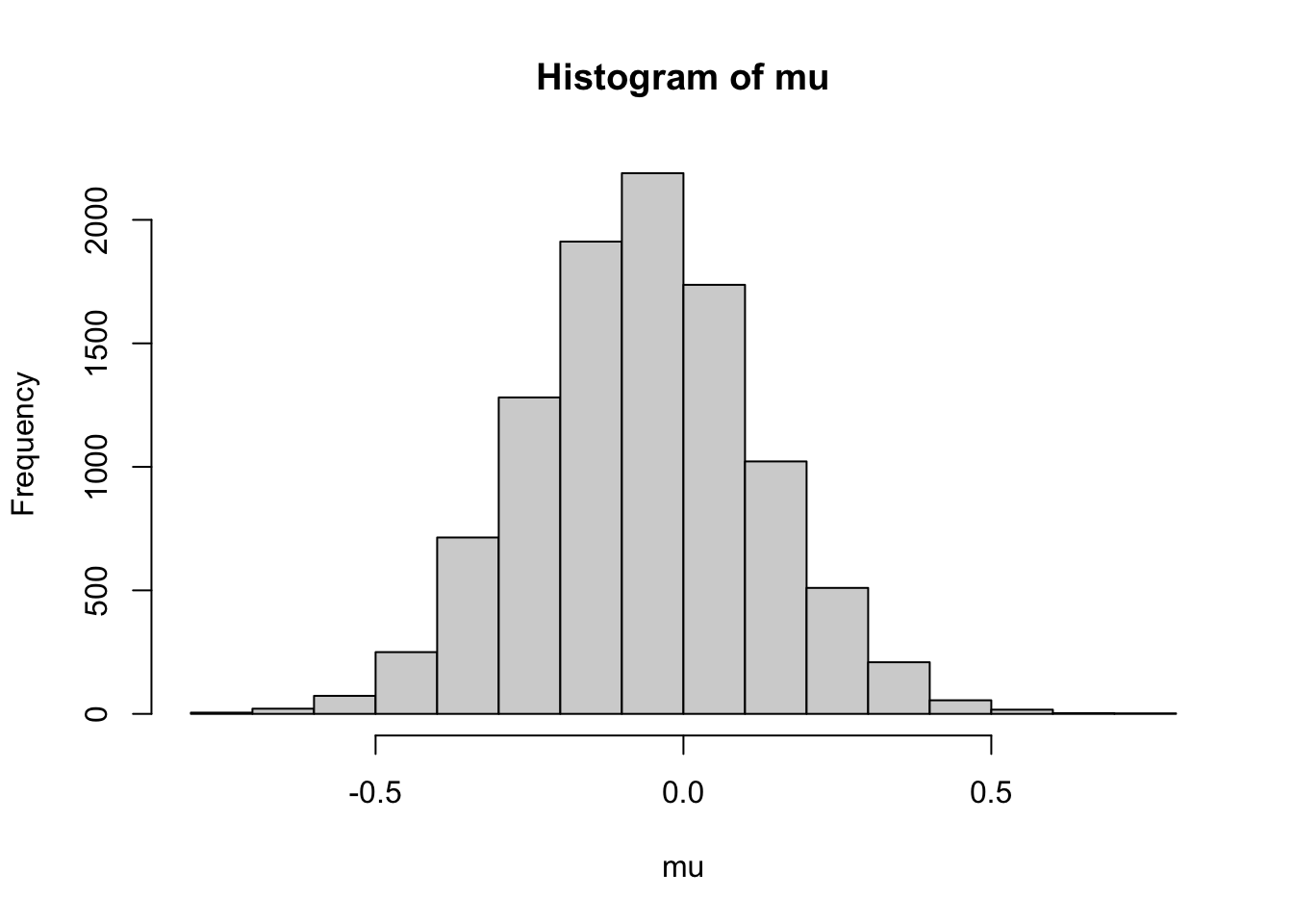
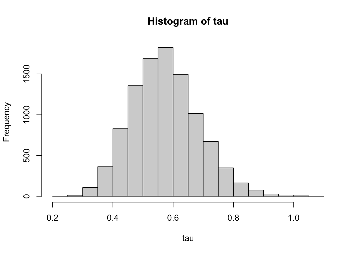
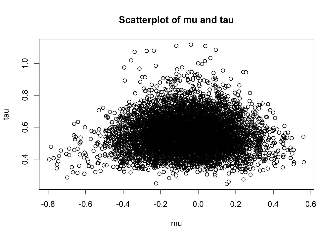
Plot samples from the joint distribution over \((\mu,\tau)\) on a scatter plot. Plot histograms for marginal \(\mu\) and \(\tau\) (marginal distributions).
Solution: First we write the joint distribution of \((y,\tau,\mu)\) as \[\begin{align*}
p(y,\tau,\mu) &= p(y|\tau,\mu) p(\mu) p(\tau)\\
&=\left(\prod_{i=1}^{n} \frac{\sqrt{\tau}}{\sqrt{2\pi}} e^{-\frac{\tau}{2}(y_i-\mu)^2} \right) \frac{1}{\sqrt{2\pi}} e^{-\frac{1}{2}\mu^2} \frac{1}{\Gamma(2)} \tau e^{-\tau}
\end{align*}\] Therefore, \[\begin{align*}
p(\mu|\tau,y) &= \frac{p(y,\tau,\mu)}{p(\tau,y)}\\
&\propto \left(\prod_{i=1}^{n} e^{-\frac{\tau}{2}(y_i-\mu)^2} \right) e^{-\frac{1}{2}\mu^2}\\
&\propto e^{-\frac{\tau n+1}{2}\mu^2 + \tau n\bar{y}\mu}\\
&\sim N\left(\frac{\tau n \bar{y}}{1+\tau n}, \frac{1}{1+\tau n}\right)\\
p(\tau|\mu, y) &= \frac{p(y,\tau,\mu)}{p(\mu,y)}\\
&\propto \left(\prod_{i=1}^{n} \sqrt{\tau}e^{-\frac{\tau}{2}(y_i-\mu)^2} \right) \tau e^{-\tau}\\
&= \tau^{1+n/2} e^{-(1+\sum_{i=1}^{n}(y_i-\mu)^2/2)\tau}\\
&\sim \mathrm{Gamma}\left(2+\frac{n}{2}, 1+\frac{1}{2}\sum_{i=1}^{n}(y_i-\mu)^2\right)
\end{align*}\]
d =read.table("https://www.dropbox.com/scl/fi/l3ao8lnfj4hwhqzjitahv/MCMCexampleData.txt?rlkey=ht4a6har3ctvphtj6o1xlggm9&dl=1")y =c(as.matrix(d))ybar =mean(y)m =10000mu =rep(0,m)tau =rep(0,m)mu[1] =0tau[1] =1for (i in2:m){ mu[i] =rnorm(1,tau[i-1]*sum(y)/(1+length(y)*tau[i-1]),sqrt(1/(1+length(y)*tau[i-1]))) tau[i] =rgamma(1,2+length(y)/2,1+sum((y-mu[i])^2)/2)}hist(mu,main="Histogram of mu")
hist(tau,main="Histogram of tau")
plot(mu,tau,main="Scatterplot of mu and tau")
Exercise 2 (Metropolis Hastings for Marketing Mix Model) Estimate parameters for the same MMM model using the Metropolis-Hastings algorithm. Assume the same state-space representation as in the previous exercise. Implement the Metropolis-Hastings algorithm for the posterior \(\mu,\tau | y\). Use normal proposal distributions for both parameters. How size of the variance of your proposal distribution affects the convergence of the algorithm?