Bayes AI
Unit 3: Bayesian Inference with Conjugate Pairs

Vadim Sokolov
George Mason University
Spring 2025
EPL Odds

English Premier League: EPL
Calculate Odds for the possible scores in a match? \[ 0-0, \; 1-0, \; 0-1, \; 1-1, \; 2-0, \ldots \] Let \(X=\) Goals scored by Arsenal
\(Y=\) Goals scored by Liverpool
What’s the odds of a team winning? \(\; \; \; P \left ( X> Y \right )\) Odds of a draw? \(\; \; \; P \left ( X = Y \right )\)
z1 = rpois(100,0.6) z2 = rpois(100,1.4) sum(z1<z2)/100 # Team 2 wins sum(z1=z2)/100 # Draw
Chelsea EPL 2017
Let’s take a historical set of data on scores Then estimate \(\lambda\) with the sample mean of the home and away scores
| home team | results | visit team | |
|---|---|---|---|
| Chelsea | 2 | 1 | West Ham |
| Chelsea | 5 | 1 | Sunderland |
| Watford | 1 | 2 | Chelsea |
| Chelsea | 3 | 0 | Burnley |
| \(\dots\) |
EPL Chelsea


Our Poisson model fits the empirical data!!
EPL: Attack and Defense Strength
Each team gets an “attack” strength and “defense” weakness rating Adjust home and away average goal estimates
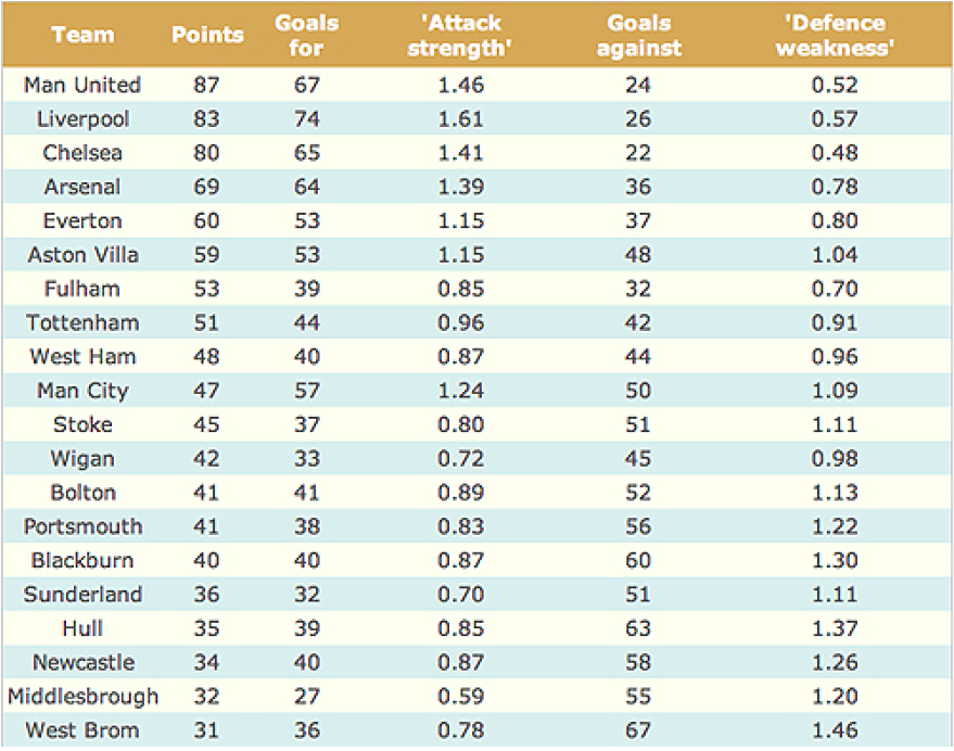
EPL: Hull vs ManU: Poisson Distribution
ManU Average away goals \(=1.47\). Prediction: \(1.47 \times 1.46 \times 1.37 = 2.95\)
Attack strength times Hull’s defense weakness times average
Hull Average home goals \(=1.47\). Prediction: \(1.47 \times 0.85 \times 0.52 = 0.65\). Simulation
| Team | Expected Goals | 0 | 1 | 2 | 3 | 4 | 5 |
|---|---|---|---|---|---|---|---|
| Man U | 2.95 | 7 | 22 | 26 | 12 | 11 | 13 |
| Hull City | 0.65 | 49 | 41 | 10 | 0 | 0 | 0 |
EPL Predictions
A model is only as good as its predictions
In our simulation Man U wins 88 games out of 100, we should bet when odds ratio is below 88 to 100.
Most likely outcome is 0-3 (12 games out of 100)
The actual outcome was 0-1 (they played on August 27, 2016)
In out simulation 0-1 was the fourth most probable outcome (9 games out of 100)
Hierarchical Distributions
Bayesian Methods
Modern Statistical/Machine Learning
- Bayes Rule and Probabilistic Learning
- Computationally challenging: MCMC and Particle Filtering
- Many applications in Finance:
Asset pricing and corporate finance problems.
Lindley, D.V. Making Decisions
Bernardo, J. and A.F.M. Smith Bayesian Theory
Bayesian Books
Hierarchical Models and MCMC
Bayesian Nonparametrics
Machine Learning
- Dynamic State Space Models \(\ldots\)
Popular Books
McGrayne (2012): The Theory that would not Die
History of Bayes-Laplace
Code breaking
Bayes search: Air France \(\ldots\)
Nate Silver: 538 and NYT
Silver (2012): The Signal and The Noise
Presidential Elections
Bayes dominant methodology
Predicting College Basketball/Oscars \(\ldots\)

Things to Know
Explosion of Models and Algorithms starting in 1950s
Bayesian Regularisation and Sparsity
Hierarchical Models and Shrinkage
Hidden Markov Models
Nonlinear Non-Gaussian State Space Models
Algorithms
Monte Carlo Method (von Neumann and Ulam, 1940s)
Metropolis-Hastings (Metropolis, 1950s)
Gibbs Sampling (Geman and Geman, Gelfand and Smith, 1980s)
Sequential Particle Filtering
Probabilistic Reasoning
- Bayesian Probability (Ramsey, 1926, de Finetti, 1931)
- Beta-Binomial Learning: Black Swans
- Elections: Nate Silver
- Baseball: Kenny Lofton and Derek Jeter
- Monte Carlo (von Neumann and Ulam, Metropolis, 1940s)
- Shrinkage Estimation (Lindley and Smith, Efron and Morris, 1970s)
Bayesian Inference
Key Idea: Explicit use of probability for summarizing uncertainty.
A probability distribution for data given parameters \[ f(y| \theta ) \; \; \text{Likelihood} \]
A probability distribution for unknown parameters \[ p(\theta) \; \; \text{Prior} \]
Inference for unknowns conditional on observed data
Inverse probability (Bayes Theorem);
Formal decision making (Loss, Utility)
Posterior Inference
Bayes theorem to derive posterior distributions \[ \begin{aligned} p( \theta | y ) & = \frac{p(y| \theta)p( \theta)}{p(y)} \\ p(y) & = \int p(y| \theta)p( \theta)d \theta \end{aligned} \] Allows you to make probability statements
- They can be very different from p-values!
Hypothesis testing and Sequential problems
- Markov chain Monte Carlo (MCMC) and Filtering (PF)
Coin Example
- What if we gamble against unfair coin flips or the person who performs the flips is trained to get the side he wants?
- In this case, we need to estimate the probability of heads \(\theta\) from the data. Suppose we have observed 10 flips \[ y = \{H, T, H, H, H, T, H, T, H, H\}, \]
- The frequency-based answer would be \(\theta = 3/10 = 0.3\), but this is not a good estimate.
Coin Example
- Bayes approach gives us more flexibility.
- Prior belief: the coin is fair, but we are not sure.
- We can model this belief by a prior distribution, we discretize the variable
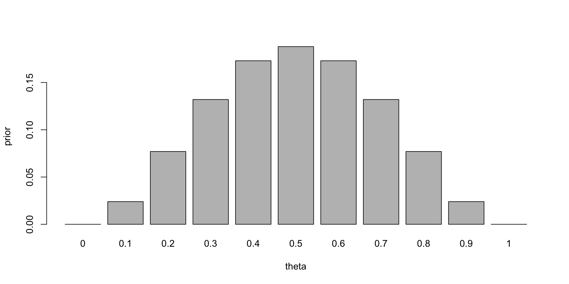
Prior distribution
Coin Example
Use Bayes rule to update our prior belief. The posterior distribution is given by \[ p(\theta \mid y) = \frac{p(y \mid \theta) p(\theta)}{p(y)}. \] The denominator is the marginal likelihood, which is given by \[ p(y) = \sum_{\theta} p(y \mid \theta) p(\theta). \] The likelihood is given by the Binomial distribution \[ p(y \mid \theta) \propto \theta^3 (1 - \theta)^7. \]
Notice, that the posterior distribution depends only on the number of positive and negative cases. Those numbers are sufficient for the inference about \(\theta\). The posterior distribution is given by
Likelihood
The likelihood is given by the Binomial distribution
Code
th = seq(0,1,length=100)
par(mar=c(4,4,0,0), bty='n')
ll = th^30*(1-th)^70; ll = ll/sum(ll)
plot(th,ll, type='l', col=1, ylab='likelihood', xlab='theta')
ll = th^3*(1-th)^7; ll = ll/sum(ll)
lines(th,ll, type='l', col=2)
labels = c('n=100', 'n=10')
legend('topright', legend=labels, col=1:2, lty=1,bty='n')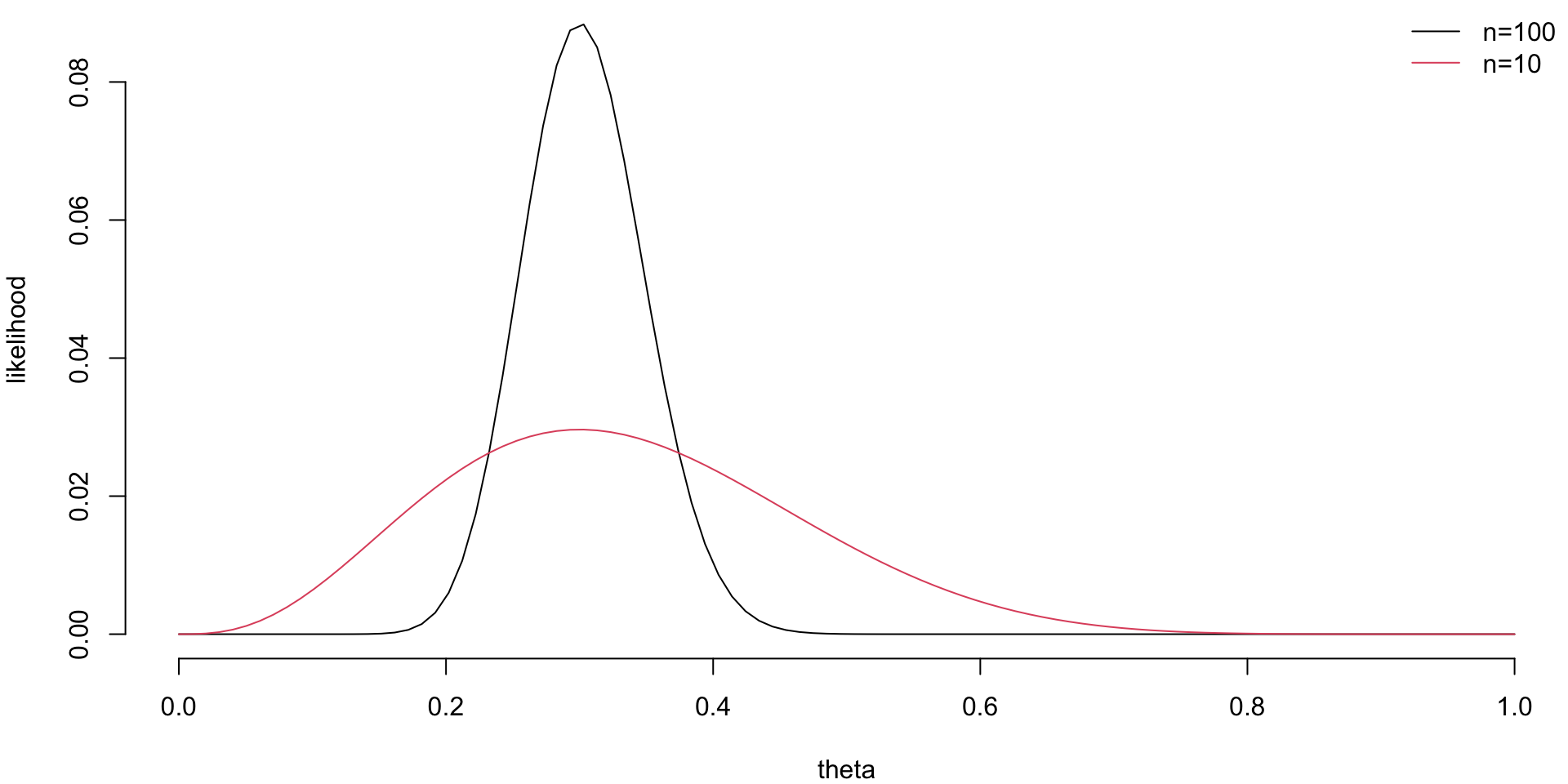
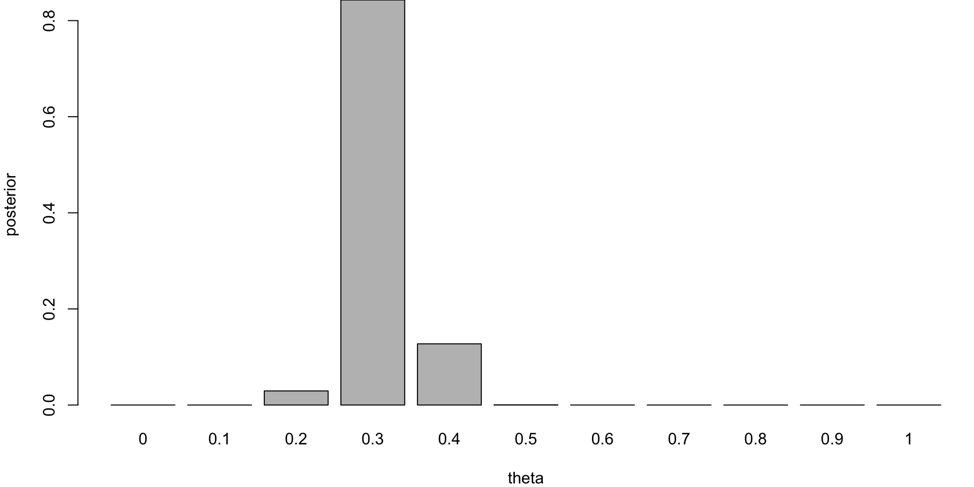
Coin Example

Posterior distribution
Coin Example
If you are to keep collecting more observations and say observe a sequence of 100 flips, then the posterior distribution will be more concentrated around the value of \(\theta = 0.3\).
Posterior distribution for n=100
This demonstrates that for large sample sizes, the frequentist approach and Bayes approach agree.
Conjugate Priors
- Definition: Let \(F\) denote the class of distributions \(f ( y | \theta )\).
A class \(\Pi\) of prior distributions is conjugate for \(F\) if the posterior distribution is in the class \(\Pi\) for all \(f \in F , \pi \in \Pi , y \in Y\).
- Example: Binomial/Beta:
Suppose that \(Y_1 , \ldots , Y_n \sim Ber ( p )\).
Let \(p \sim Beta ( \alpha , \beta )\) where \(( \alpha , \beta )\) are known hyper-parameters.
The beta-family is very flexible
Prior mean \(E ( p ) = \frac{\alpha}{ \alpha + \beta }\).
Bayes Learning: Beta-Binomial
How do I update my beliefs about a coin toss?
Likelihood for Bernoulli \[ p\left( y|\theta\right) =\prod_{t=1}^{T}p\left( y_{t}|\theta\right) =\theta^{\sum_{t=1}^{T}y_{t}}\left( 1-\theta\right) ^{T-\sum_{t=1}^{T}y_{t}}. \] Initial prior distribution \(\theta\sim\mathcal{B}\left( a,A\right)\) given by \[ p\left( \theta|a,A\right) =\frac{\theta^{a-1}\left( 1-\theta\right) ^{A-1}}{B\left( a,A\right) } \]
Bayes Learning: Beta-Binomial
Updated posterior distribution is also Beta \[ p\left( \theta|y\right) \sim\mathcal{B}\left( a_{T},A_{T}\right) \; {\rm and} \; a_{T}=a+\sum_{t=1}^{T}y_{t} , A_{T}=A+T-\sum_{t=1}^{T}y_{t} \] The posterior mean and variance are \[ E\left[ \theta|y\right] =\frac{a_{T}}{a_{T}+A_{T}}\text{ and }var\left[ \theta|y\right] =\frac{a_{T}A_{T}}{\left( a_{T}+A_{T}\right) ^{2}\left( a_{T}+A_{T}+1\right) } \]
Binomial-Beta
\(p ( p | \bar{y} )\) is the posterior distribution for \(p\)
\(\bar{y}\) is a sufficient statistic.
Bayes theorem gives \[ \begin{aligned} p ( p | y ) & \propto f ( y | p ) p ( p | \alpha , \beta )\\ & \propto p^{\sum y_i} (1 - p )^{n - \sum y_i } \cdot p^{\alpha - 1} ( 1 - p )^{\beta - 1} \\ & \propto p^{ \alpha + \sum y_i - 1 } ( 1 - p )^{ n - \sum y_i + \beta - 1} \\ & \sim Beta ( \alpha + \sum y_i , \beta + n - \sum y_i ) \end{aligned} \]
The posterior mean is a shrinkage estimator
Combination of sample mean \(\bar{y}\) and prior mean \(E( p )\)
\[ E(p|y) = \frac{\alpha + \sum_{i=1}^n y_i}{\alpha + \beta + n} = \frac{n}{n+ \alpha +\beta} \bar{y} + \frac{\alpha + \beta}{\alpha + \beta+n} \frac{\alpha}{\alpha+\beta} \]
Binomial-Beta
Let \(p_i\) be the death rate proportion under treatment \(i\).
To compare treatment \(A\) to \(B\) directly compute \(P ( p_1 > p_2 | D )\).
Prior \(beta ( \alpha , \beta )\) with prior mean \(E ( p ) = \frac{\alpha}{\alpha + \beta }\).
Posterior \(beta ( \alpha + \sum x_i , \beta + n - \sum x_i )\)
- For \(A\), \(beta ( 1 , 1 ) \rightarrow beta ( 8 , 94 )\)
For \(B\), \(beta ( 1 , 1 ) \rightarrow beta ( 2 , 100 )\)
- Inference: \(P ( p_1 > p_2 | D ) \approx 0.98\)
Black Swans
Taleb, The Black Swan: the Impact of the Highly Improbable
Suppose you’re only see a sequence of White Swans, having never seen a Black Swan.
What’s the Probability of Black Swan event sometime in the future?
Suppose that after \(T\) trials you have only seen successes \(( y_1 , \ldots , y_T ) = ( 1 , \ldots , 1 )\). The next trial being a success has \[ p( y_{T+1} =1 | y_1 , \ldots , y_T ) = \frac{T+1}{T+2} \] For large \(T\) is almost certain. Here \(a=A=1\).
Black Swans
Principle of Induction (Hume)
The probability of never seeing a Black Swan is given by \[ p( y_{T+1} =1 , \ldots , y_{T+n} = 1 | y_1 , \ldots , y_T ) = \frac{ T+1 }{ T+n+1 } \rightarrow 0 \]
Black Swan will eventually happen – don’t be surprised when it actually happens.
Bayesian Learning: Poisson-Gamma
Poisson/Gamma: Suppose that \(Y_1 , \ldots , Y_n \mid \lambda \sim Poi ( \lambda )\).
Let \(\lambda \sim Gamma ( \alpha , \beta )\)
\(( \alpha , \beta )\) are known hyper-parameters.
- The posterior distribution is
\[ \begin{aligned} p ( \lambda | y ) & \propto \exp ( - n \lambda ) \lambda^{ \sum y_i } \lambda^{ \alpha - 1 } \exp ( - \beta \lambda ) \\ & \sim Gamma ( \alpha + \sum y_i , n + \beta ) \end{aligned} \]
Example: Clinical Trials
Novick and Grizzle: A Bayesian Approach to the Analysis of Data from Clinical Trials
Four treatments for duodenal ulcers.
Doctors assess the state of the patient.
Sequential data
(\(\alpha\)-spending function, can only look at presanctified times).
| Treat | Excellent | Fair | Death |
|---|---|---|---|
| A | 76 | 17 | 7 |
| B | 89 | 10 | 1 |
| C | 86 | 13 | 1 |
| D | 88 | 9 | 3 |
Conclusion: Cannot reject at the 5% level
Conjugate Gamma - Poisson model+sensitivity analysis.
Sensitivity Analysis
Important to do a sensitivity analysis.
| Treat | Excellent | Fair | Death |
|---|---|---|---|
| A | 76 | 17 | 7 |
| B | 89 | 10 | 1 |
| C | 86 | 13 | 1 |
| D | 88 | 9 | 3 |
Poisson-Gamma, prior \(\Gamma ( m , z)\) and \(\lambda_i\) be the expected death rate.
\(\lambda_i\) is the death reate of treatment \(i\).
Compute \(P \left ( \frac{ \lambda_1 }{ \lambda_2 } > c \right )\)
| Prob | ( 0 , 0 ) | ( 100, 2) | ( 200 , 5) |
|---|---|---|---|
| \(P \left ( \frac{ \lambda_1 }{ \lambda_2 } > 1.3\right)\) | 0.95 | 0.88 | 0.79 |
| \(P \left ( \frac{ \lambda_1 }{ \lambda_2 } > 1.6 \right)\) | 0.91 | 0.80 | 0.64 |
Bayesian Learning: Normal-Normal
Using Bayes rule we get \[ p( \mu | y ) \propto p( y| \mu ) p( \mu ) \]
- Posterior is given by
\[ p( \mu | y ) \propto \exp \left ( - \frac{1}{2 \sigma^2} \sum_{i=1}^n ( y_i - \mu )^2 - \frac{1}{2 \tau^2} ( \mu - \mu_0 )^2 \right ) \] Hence \(\mu | y \sim N \left ( \hat{\mu}_B , V_{\mu} \right )\) where
\[ \hat{\mu}_B = \frac{ n / \sigma^2 }{ n / \sigma^2 + 1 / \tau^2 } \bar{y} + \frac{ 1 / \tau^2 }{ n / \sigma^2 + 1 / \tau^2 }\mu_0 \; \; {\rm and} \; \; V_{\mu}^{-1} = \frac{n}{ \sigma^2 } + \frac{1}{\tau^2} \] A shrinkage estimator.
SAT Scores
SAT (\(200-800\)): 8 high schools and estimate effects.
| School | Estimated \(y_j\) | St. Error \(\sigma_j\) | Average Treatment \(\theta_i\) |
|---|---|---|---|
| A | 28 | 15 | ? |
| B | 8 | 10 | ? |
| C | -3 | 16 | ? |
| D | 7 | 11 | ? |
| E | -1 | 9 | ? |
| F | 1 | 11 | ? |
| G | 18 | 10 | ? |
| H | 12 | 18 | ? |
\(\theta_j\) average effects of coaching programs
\(y_j\) estimated treatment effects, for school \(j\), standard error \(\sigma_j\).
Estimates
Two programs appear to work (improvements of 18 and 28)
Large standard errors. Overlapping Confidence Intervals?
Classical hypothesis test fails to reject the hypothesis that the \(\theta_j\)’s are equal.
Pooled estimate has standard error of \(4.2\) with
\[ \hat{\theta} = \frac{ \sum_j ( y_j / \sigma_j^2 ) }{ \sum_j ( 1 / \sigma_j^2 ) } = 7.9 \]
- Neither separate or pooled seems sensible.
Bayesian shrinkage!
Hierarchical Model
Also known as a random effects model or multi-level model.
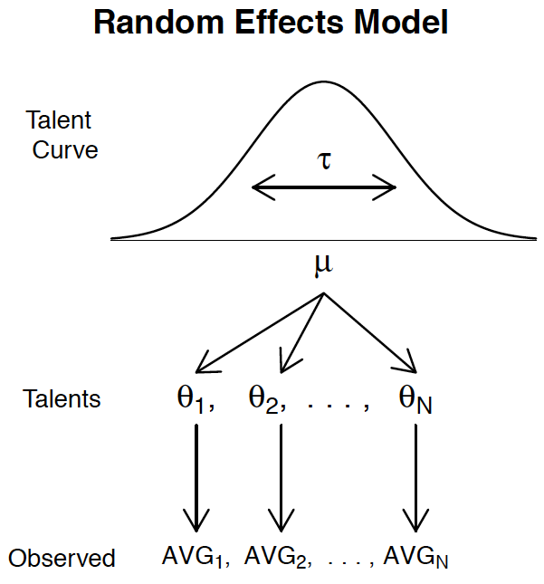
Hierarchical Model
Hierarchical Model (\(\sigma_j^2\) known) is given by \[ \bar{y}_j | \theta_j \sim N ( \theta_j , \sigma_j^2 ) \] Unequal variances–differential shrinkage.
- Prior Distribution: \(\theta_j \sim N ( \mu , \tau^2 )\) for \(1 \leq j \leq 8\).
Traditional random effects model.
Exchangeable prior for the treatment effects.
As \(\tau \rightarrow 0\) (complete pooling) and as \(\tau \rightarrow \infty\) (separate estimates).
- Hyper-prior Distribution: \(p( \mu , \tau^2 ) \propto 1 / \tau\).
The posterior \(p( \mu , \tau^2 | y )\) can be used to “estimate” \(( \mu , \tau^2 )\).
Posterior
Joint Posterior Distribution \(y = ( y_1 , \ldots , y_J )\) \[ p( \theta , \mu , \tau | y ) \propto p( y| \theta ) p( \theta | \mu , \tau )p( \mu , \tau ) \] \[ \propto p( \mu , \tau^2) \prod_{i=1}^8 N ( \theta_j | \mu , \tau^2 ) \prod_{j=1}^8 N ( y_j | \theta_j ) \] \[ \propto \tau^{-9} \exp \left ( - \frac{1}{2} \sum_j \frac{1}{\tau^2} ( \theta_j - \mu )^2 - \frac{1}{2} \sum_j \frac{1}{\sigma_j^2} ( y_j - \theta_j )^2 \right ) \] MCMC!
Posterior Inference
Report posterior quantiles
| School | 2.5% | 25% | 50% | 75% | 97.5% |
|---|---|---|---|---|---|
| A | -2 | 6 | 10 | 16 | 32 |
| B | -5 | 4 | 8 | 12 | 20 |
| C | -12 | 3 | 7 | 11 | 22 |
| D | -6 | 4 | 8 | 12 | 21 |
| E | -10 | 2 | 6 | 10 | 19 |
| F | -9 | 2 | 6 | 10 | 19 |
| G | -1 | 6 | 10 | 15 | 27 |
| H | -7 | 4 | 8 | 13 | 23 |
| \(\mu\) | -2 | 5 | 8 | 11 | 18 |
| \(\tau\) | 0.3 | 2.3 | 5.1 | 8.8 | 21 |
Schools \(A\) and \(G\) are similar!
Bayesian Shrinkage
Bayesian shrinkage provides a way of modeling complex datasets.
Baseball batting averages: Stein’s Paradox
Batter-pitcher match-up: Kenny Lofton and Derek Jeter
Bayes Elections
Toxoplasmosis
Bayes MoneyBall
Bayes Portfolio Selection
Example: Baseball
Batter-pitcher match-up?
Prior information on overall ability of a player.
Small sample size, pitcher variation.
- Let \(p_i\) denote batter’s ability. Observed number of hits \(y_i\)
\[ (y_i | p_i ) \sim Bin ( T_i , p_i ) \; \; {\rm with} \; \; p_i \sim Be ( \alpha , \beta ) \] where \(T_i\) is the number of at-bats against pitcher \(i\). A priori \(E( p_i ) = \alpha / (\alpha+\beta ) = \bar{p}_i\).
- The extra heterogeneity leads to a prior variance \(Var (p_i ) = \bar{p}_i (1 - \bar{p}_i ) \phi\) where \(\phi = ( \alpha + \beta + 1 )^{-1}\).
Sports Data: Baseball
Kenny Lofton hitting versus individual pitchers.
| Pitcher | At-bats | Hits | ObsAvg |
|---|---|---|---|
| J.C. Romero | 9 | 6 | .667 |
| S. Lewis | 5 | 3 | .600 |
| B. Tomko | 20 | 11 | .550 |
| T. Hoffman | 6 | 3 | .500 |
| K. Tapani | 45 | 22 | .489 |
| A. Cook | 9 | 4 | .444 |
| J. Abbott | 34 | 14 | .412 |
| A.J. Burnett | 15 | 6 | .400 |
| K. Rogers | 43 | 17 | .395 |
| Pitcher | At-bats | Hits | ObsAvg |
|---|---|---|---|
| A. Harang | 6 | 2 | .333 |
| K. Appier | 49 | 15 | .306 |
| R. Clemens | 62 | 14 | .226 |
| C. Zambrano | 9 | 2 | .222 |
| N. Ryan | 10 | 2 | .200 |
| E. Hanson | 41 | 7 | .171 |
| E. Milton | 19 | 1 | .056 |
| M. Prior | 7 | 0 | .000 |
| Total | 7630 | 2283 | .299 |
Baseball: Kenny Lofton
Kenny Lofton (career \(.299\) average, and current \(.308\) average for 2006 season) was facing the pitcher Milton (current record 1 for 19).
- Is putting in a weaker player really a better bet?
- Over-reaction to bad luck?
\(\mathbb{P}\left ( \leq 1 \; {\rm hit \; in \; } 19 \; {\rm attempts} | p = 0.3 \right ) = 0.01\)
An unlikely 1-in-100 event.
Baseball: Kenny Lofton
Bayes solution: shrinkage. Borrow strength across pitchers
Bayes estimate: use the posterior mean
Lofton’s batting estimates that vary from \(.265\) to \(.340\).
The lowest being against Milton.
\(.265 < .275\)
Conclusion: resting Lofton against Milton was justified!!
Bayes Batter-pitcher match-up
Here’s our model again ...
Small sample sizes and pitcher variation.
Let \(p_i\) denote Lofton’s ability. Observed number of hits \(y_i\)
\[ (y_i | p_i ) \sim Bin ( T_i , p_i ) \; \; {\rm with} \; \; p_i \sim Be ( \alpha , \beta ) \] where \(T_i\) is the number of at-bats against pitcher \(i\).
Estimate \(( \alpha , \beta )\)
Example: Derek Jeter
Derek Jeter 2006 season versus individual pitchers.
| Pitcher | At-bats | Hits | ObsAvg | EstAvg | 95% Int |
|---|---|---|---|---|---|
| R. Mendoza | 6 | 5 | .833 | .322 | (.282, .394) |
| H. Nomo | 20 | 12 | .600 | .326 | (.289, .407) |
| A.J.Burnett | 5 | 3 | .600 | .320 | (.275, .381) |
| E. Milton | 28 | 14 | .500 | .324 | (.291, .397) |
| D. Cone | 8 | 4 | .500 | .320 | (.218, .381) |
| R. Lopez | 45 | 21 | .467 | .326 | (.291, .401) |
| K. Escobar | 39 | 16 | .410 | .322 | (.281, .386) |
| J. Wettland | 5 | 2 | .400 | .318 | (.275, .375) |
Example: Derek Jeter
Derek Jeter 2006 season versus individual pitchers.
| Pitcher | At-bats | Hits | ObsAvg | EstAvg | 95% Int |
|---|---|---|---|---|---|
| T. Wakefield | 81 | 26 | .321 | .318 | (.279, .364) |
| P. Martinez | 83 | 21 | .253 | .312 | (.254, .347) |
| K. Benson | 8 | 2 | .250 | .317 | (.264, .368) |
| T. Hudson | 24 | 6 | .250 | .315 | (.260, .362) |
| J. Smoltz | 5 | 1 | .200 | .314 | (.253, .355) |
| F. Garcia | 25 | 5 | .200 | .314 | (.253, .355) |
| B. Radke | 41 | 8 | .195 | .311 | (.247, .347) |
| D. Kolb | 5 | 0 | .000 | .316 | (.258, .363) |
| J. Julio | 13 | 0 | .000 | .312 | (.243, .350 ) |
| Total | 6530 | 2061 | .316 |
Bayes Estimates
- Stern estimates \(\hat{\phi} = ( \alpha + \beta + 1 )^{-1} = 0.002\) for Jeter
- Doesn’t vary much across the population of pitchers.
- The extremes are shrunk the most also matchups with the smallest sample sizes.
- Jeter had a season \(.308\) average.
Bayes estimates vary from \(.311\) to \(.327\)–he’s very consistent.
If all players had a similar record then a constant batting average would make sense.
Bayes Elections: Nate Silver: Multinomial-Dirichlet
Predicting the Electoral Vote (EV)
- Multinomial-Dirichlet: \((\hat{p} | p) \sim Multi (p), ( p | \alpha ) \sim Dir (\alpha)\)
\[ p_{Obama} = ( p_{1}, \ldots ,p_{51} | \hat{p}) \sim Dir \left ( \alpha + \hat{p} \right ) \]
- Flat uninformative prior \(\alpha\equiv 1\).
http://www.electoral-vote.com/evp2012/Pres/prespolls.csv
Bayes Elections: Nate Silver: Simulation
Calculate probabilities via simulation: rdirichlet \[
p \left ( p_{j,O} | {\rm data} \right ) \;\; {\rm and} \; \;
p \left ( EV >270 | {\rm data} \right )
\]
The election vote prediction is given by the sum \[ EV =\sum_{j=1}^{51} EV(j) \mathbb{E} \left ( p_{j} | {\rm data} \right ) \] where \(EV(j)\) are for individual states
Polling Data
Electoral Vote (EV), Polling Data: Mitt and Obama percentages
| State | M.pct | O.pct | EV |
|---|---|---|---|
| Alabama | 58 | 36 | 9 |
| Alaska | 55 | 37 | 3 |
| Arizona | 50 | 46 | 10 |
| Arkansas | 51 | 44 | 6 |
| California | 33 | 55 | 55 |
| Colorado | 45 | 52 | 9 |
| Connecticut | 31 | 56 | 7 |
| Delaware | 38 | 56 | 3 |
| D.C. | 13 | 82 | 3 |
| Florida | 46 | 50 | 27 |
| Georgia | 52 | 47 | 15 |
| Hawaii | 32 | 63 | 4 |
| Idaho | 68 | 26 | 4 |
| State | M.pct | O.pct | EV |
|---|---|---|---|
| Illinois | 35 | 59 | 21 |
| Indiana | 48 | 48 | 11 |
| Iowa | 37 | 54 | 7 |
| Kansas | 63 | 31 | 6 |
| Kentucky | 51 | 42 | 8 |
| Louisiana | 50 | 43 | 9 |
| Maine | 35 | 56 | 4 |
| Maryland | 39 | 54 | 10 |
| Massachusetts | 34 | 53 | 12 |
| Michigan | 37 | 53 | 17 |
| Minnesota | 42 | 53 | 10 |
| Mississippi | 46 | 33 | 6 |
Polling Data:


Chicago Bears 2014-2015 Season
Bayes Learning: Update our beliefs in light of new information
- In the 2014-2015 season.
The Bears suffered back-to-back 50-points defeats.
Partiots-Bears \(51-23\)
Packers-Bears \(55-14\)
- Their next game was at home against the Minnesota Vikings.
Current line against the Vikings was \(-3.5\) points.
Slightly over a field goal
What’s the Bayes approach to learning the line?
Hierarchical Model
Hierarchical model for the current average win/lose this year \[ \begin{aligned} \bar{y} | \theta & \sim N \left ( \theta , \frac{\sigma^2}{n} \right ) \sim N \left ( \theta , \frac{18.34^2}{9} \right )\\ \theta & \sim N( 0 , \tau^2 ) \end{aligned} \] Here \(n =9\) games so far. With \(s = 18.34\) points
Pre-season prior mean \(\mu_0 = 0\), standard deviation \(\tau = 4\).
Record so-far. Data \(\bar{y} = -9.22\).
Chicago Bears
Bayes Shrinkage estimator \[ \mathbb{E} \left ( \theta | \bar{y} , \tau \right ) = \frac{ \tau^2 }{ \tau^2 + \frac{\sigma^2}{n} } \bar{y} \]
The Shrinkage factor is \(0.3\)!!
That’s quite a bit of shrinkage. Why?
- Our updated estimator is
\[ \mathbb{E} \left ( \theta | \bar{y} , \tau \right ) = - 2.75 > -.3.5 \] where current line is \(-3.5\).
- Based on our hierarchical model this is an over-reaction.
One point change on the line is about 3% on a probability scale.
Alternatively, calculate a market-based \(\tau\) given line \(=-3.5\).
Chicago Bears
Last two defeats were 50 points scored by opponent (2014-15)
[1] -9.222222[1] 18.34242[1] 0.2997225[1] 0.4390677Home advantage is worth 3 points. Vikings an average record.
Result: Bears 21, Vikings 13
Stein’s Estimator
- Popularized by Efron’s 1970 paper
- Discovered by Charles Stein in 1956 and further developed with James in 1961 (James-Stein estimator)
- Want to estimate \(p\) means of several independent normal distributions simultaneously. \[ \mu_1, \mu_2,\ldots,\mu_p \]
- MLE: \(\mu_i\) is simply the sample observation \(x_i\) from the i-th distribution, considering each mean individually.
The Shocking Result (Stein Paradox)
- When \(p>3\) there is different estimator that is uniformly better than using the individual sample means (\(x_1\), \(x_2\), …, \(x_p\)) when you consider the total squared error risk across all means.
- “Uniformly better” means it’s better for all possible true values of the means (\(\mu_1\), \(\mu_2\), …, \(\mu_p\)).
- The distributions are assumed to be independent.
- Sample means are individually good estimators.
Counterintuitive! How can we improve upon something that already seems so natural and optimal when considered in isolation?
The James-Stein Estimator
The estimator that Stein and James proposed (often called the James-Stein estimator or shrinkage estimator) is of the form: \[ \mu_{JS} = (1 - b)\hat x \] - \(b\) is a “shrinkage factor” calculated based on the data, typically something like \(b = (p - 2) S^2 / ||x||^2\), where \(S^2\) is the variance of the underlying distributions (often assumed to be known or estimated), and \(||x||\) is the Euclidean norm of \(x\).
What does this estimator do?
- It shrinks the original estimate \(\mu\) towards the origin (zero vector). The amount of shrinkage is determined by the data itself. If \(||x||^2\) is large (observations are far from zero), the shrinkage factor
bis smaller, and less shrinkage is applied. If \(||x||^2\) is small, \(b\) is larger, and more shrinkage is applied towards zero. - Brad Efron’s 1970 paper, “Stein’s Paradox in Statistics,” published in the American Statistician, simplified and clarified the paradox
- Geometric Interpretation: Efron emphasized a geometric perspective on the Stein Paradox.
- Risk Decomposition and Analysis: derivation cleverly decomposed the risk (expected squared error) of the estimators. This decomposition clearly showed how the James-Stein estimator reduces risk compared to the standard estimator, especially in higher dimensions.
Risk Analysis and Decomposition
\[ Risk(\mu_{JS}) = E[ ||\mu_{JS}(x) - \mu||^2 ] = E\left[ \sum_{i=1}^p (\mu_{JS,i}(x) - \mu_i)^2 \right] \] - Each component of \(x - \mu\) has variance \(\sigma^2\) (let’s assume for simplicity all distributions have the same known variance ^2).
Say \(\mu_{JS}(x) = x\), the risk becomes: \[ Risk(x) = E[ ||x - \mu||^2 ] = E\left[ \sum_{i=1}^p (x_i - \mu_i)^2 \right] = \sum_{i=1}^p Var(x) = p\sigma^2 \] This is the risk of the standard MLE estimator. It scales linearly with the dimension p.
Risk of a Shrinkage Estimator
\[ \mu_{JS} = (1 - b)x \] where b is a fixed constant between 0 and 1. Efron then analyzes the risk of this estimator: \[ Risk(\mu_{JS}) = E[ ||(1 - b)x - \mu||^2 ] = E[ ||(1 - b)(x - \mu) - b\mu||^2 ] \] By expanding this using vector algebra and expectations, and making use of the independence and normality assumptions, Efron shows that you can decompose the risk into terms related to b and the dimension p.
Risk of a Shrinkage Estimator
Approximately optimal fixed shrinkage constant b is around \[ (p - 2) / E[||x||^2] \] or proportional to \((p-2) / ||x||^2\) in the data-dependent version.
Stein’s Paradox
Stein paradox: possible to make a uniform improvement on the MLE in terms of MSE.
- Mistrust of the statistical interpretation of Stein’s result.
In particular, the loss function.
Difficulties in adapting the procedure to special cases
Long familiarity with good properties for the MLE
Any gains from a “complicated” procedure could not be worth the extra trouble (Tukey, savings not more than 10 % in practice)
For \(k\ge 3\), we have the remarkable inequality \[ MSE(\hat \theta_{JS},\theta) < MSE(\bar y,\theta) \; \forall \theta \] Bias-variance explanation! Inadmissability of the classical stats.
Baseball Batting Averages
Data: 18 major-league players after 45 at bats (1970 season)
| Player | \(\bar{y}_i\) | \(E ( p_i | D )\) | average season |
|---|---|---|---|
| Clemente | 0.400 | 0.290 | 0.346 |
| Robinson | 0.378 | 0.286 | 0.298 |
| Howard | 0.356 | 0.281 | 0.276 |
| Johnstone | 0.333 | 0.277 | 0.222 |
| Berry | 0.311 | 0.273 | 0.273 |
| Spencer | 0.311 | 0.273 | 0.270 |
| Kessinger | 0.311 | 0.268 | 0.263 |
| Alvarado | 0.267 | 0.264 | 0.210 |
| Santo | 0.244 | 0.259 | 0.269 |
| Swoboda | 0.244 | 0.259 | 0.230 |
| Unser | 0.222 | 0.254 | 0.264 |
| Williams | 0.222 | 0.254 | 0.256 |
| Scott | 0.222 | 0.254 | 0.303 |
| Petrocelli | 0.222 | 0.254 | 0.264 |
| Rodriguez | 0.222 | 0.254 | 0.226 |
| Campanens | 0.200 | 0.259 | 0.285 |
| Munson | 0.178 | 0.244 | 0.316 |
| Alvis | 0.156 | 0.239 | 0.200 |
Baseball Data: First Shrinkage Estimator: Efron and Morris

Baseball Shrinkage
Shrinkage
Let \(\theta_i\) denote the end of season average
- Lindley: shrink to the overall grand mean
\[ c = 1 - \frac{ ( k - 3 ) \sigma^2 }{ \sum ( \bar{y}_i - \bar{y} )^2 } \] where \(\bar{y}\) is the overall grand mean and
\[ \hat{\theta} = c \bar{y}_i + ( 1 - c ) \bar{y} \]
- Baseball data: \(c = 0.212\) and \(\bar{y} = 0.265\).
Compute \(\sum ( \hat{\theta}_i - \bar{y}^{obs}_i )^2\) and see which is lower: \[ MLE = 0.077 \; \; STEIN = 0.022 \] That’s a factor of \(3.5\) times better!
Batting Averages

Baseball Paradoxes
Shrinkage on Clemente too severe: \(z_{Cl} = 0.265 + 0.212 ( 0.400 - 0.265) = 0.294\).
The \(0.212\) seems a little severe
Limited translation rules, maximum shrinkage eg. 80%
Not enough shrinkage eg O’Connor ( \(y = 1 , n = 2\)). \(z_{O'C} = 0.265 + 0.212 ( 0.5 - 0.265 ) = 0.421\).
Still better than Ted Williams \(0.406\) in 1941.
Foreign car sales (\(k = 19\)) will further improve MSE performance! It will change the shrinkage factors.
Clearly an improvement over the Stein estimator is
\[ \hat{\theta}_{S+} = \max \left ( \left ( 1 - \frac{k-2}{ \sum \bar{Y}_i^2 } \right ) , 0 \right ) \bar{Y}_i \]
Baseball Prior
- Include extra prior knowledge
- Empirical distribution of all major league players \[ \theta_i \sim N ( 0.270 , 0.015 ) \]
- The 0.270 provides another origin to shrink to and the prior variance 0.015 would give a different shrinkage factor.
- To fully understand maybe we should build a probabilistic model and see what the posterior mean is as our estimator for the unknown parameters.
Shrinkage: Unequal Variances
Model \(Y_i | \theta_i \sim N ( \theta_i , D_i )\) where \(\theta_i \sim N ( \theta_0 , A ) \sim N ( 0.270 , 0.015 )\).
The \(D_i\) can be different – unequal variances
Bayes posterior means are given by
\[ E ( \theta_i | Y ) = ( 1 - B_i ) Y_i \; \; {\rm where} \; \; B_i = \frac{ D_i }{ D_i + A } \] where \(\hat{A}\) is estimated from the data, see Efron and Morris (1975).
- Different shrinkage factors as different variances \(D_i\).
\(D_i \propto n_i^{-1}\) and so smaller sample sizes are shrunk more.
Makes sense.
Example: Toxoplasmosis Data
Disease of Blood that is endemic in tropical regions.
Data: 5000 people in El Salvador (varying sample sizes) from 36 cities.
Estimate “true” prevalences \(\theta_i\) for \(1 \leq i \leq 36\)
Allocation of Resources: should we spend funds on the city with the highest observed occurrence of the disease? Same shrinkage factors?
Shrinkage Procedure (Efron and Morris, p315) \[ z_i = c_i y_i \] where \(y_i\) are the observed relative rates (normalized so \(\bar{y} = 0\) The smaller sample sizes will get shrunk more.
The most gentle are in the range \(0.6 \rightarrow 0.9\) but some are \(0.1 \rightarrow 0.3\).
Bayes Portfolio Selection
de Finetti and Markowitz: Mean-variance portfolio shrinkage: \(\frac{1}{\gamma} \Sigma^{-1} \mu\)
Different shrinkage factors for different history lengths.
Portfolio Allocation in the SP500 index
Entry/exit; splits; spin-offs etc. For example, 73 replacements to the SP500 index in period 1/1/94 to 12/31/96.
Advantage: \(E ( \alpha | D_t ) = 0.39\), that is 39 bps per month which on an annual basis is \(\alpha = 468\) bps.
The posterior mean for \(\beta\) is \(p ( \beta | D_t ) = 0.745\)
\(\bar{x}_{M} = 12.25 \%\) and \(\bar{x}_{PT} = 14.05 \%\).
SP Composition
| Date | Symbol | 6/96 | 12/89 | 12/79 | 12/69 |
|---|---|---|---|---|---|
| General Electric | GE | 2.800 | 2.485 | 1.640 | 1.569 |
| Coca Cola | KO | 2.342 | 1.126 | 0.606 | 1.051 |
| Exxon | XON | 2.142 | 2.672 | 3.439 | 2.957 |
| ATT | T | 2.030 | 2.090 | 5.197 | 5.948 |
| Philip Morris | MO | 1.678 | 1.649 | 0.637 | ***** |
| Royal Dutch | RD | 1.636 | 1.774 | 1.191 | ***** |
| Merck | MRK | 1.615 | 1.308 | 0.773 | 0.906 |
| Microsoft | MSFT | 1.436 | ***** | ***** | ***** |
| Johnson/Johnson | JNJ | 1.320 | 0.845 | 0.689 | ***** |
| Intel | INTC | 1.262 | ***** | ***** | ***** |
| Procter and Gamble | PG | 1.228 | 1.040 | 0.871 | 0.993 |
| Walmart | WMT | 1.208 | 1.084 | ***** | ***** |
| IBM | IBM | 1.181 | 2.327 | 5.341 | 9.231 |
| Hewlett Packard | HWP | 1.105 | 0.477 | 0.497 | ***** |
SP Composition
| Date | Symbol | 6/96 | 12/89 | 12/79 | 12/69 |
|---|---|---|---|---|---|
| Pepsi | PEP | 1.061 | 0.719 | ***** | ***** |
| Pfizer | PFE | 0.918 | 0.491 | 0.408 | 0.486 |
| Dupont | DD | 0.910 | 1.229 | 0.837 | 1.101 |
| AIG | AIG | 0.910 | 0.723 | ***** | ***** |
| Mobil | MOB | 0.906 | 1.093 | 1.659 | 1.040 |
| Bristol Myers Squibb | BMY | 0.878 | 1.247 | ***** | 0.484 |
| GTE | GTE | 0.849 | 0.975 | 0.593 | 0.705 |
| General Motors | GM | 0.848 | 1.086 | 2.079 | 4.399 |
| Disney | DIS | 0.839 | 0.644 | ***** | ***** |
| Citicorp | CCI | 0.831 | 0.400 | 0.418 | ***** |
| BellSouth | BLS | 0.822 | 1.190 | ***** | ***** |
| Motorola | MOT | 0.804 | ***** | ***** | ***** |
| Ford | F | 0.798 | 0.883 | 0.485 | 0.640 |
| Chervon | CHV | 0.794 | 0.990 | 1.370 | 0.966 |
SP Composition
| Date | Symbol | 6/96 | 12/89 | 12/79 | 12/69 |
|---|---|---|---|---|---|
| Amoco | AN | 0.733 | 1.198 | 1.673 | 0.758 |
| Eli Lilly | LLY | 0.720 | 0.814 | ***** | ***** |
| Abbott Labs | ABT | 0.690 | 0.654 | ***** | ***** |
| AmerHome Products | AHP | 0.686 | 0.716 | 0.606 | 0.793 |
| FedNatlMortgage | FNM | 0.686 | ***** | ***** | ***** |
| McDonald’s | MCD | 0.686 | 0.545 | ***** | ***** |
| Ameritech | AIT | 0.639 | 0.782 | ***** | ***** |
| Cisco Systems | CSCO | 0.633 | ***** | ***** | ***** |
| CMB | CMB | 0.621 | ***** | ***** | ***** |
| SBC | SBC | 0.612 | 0.819 | ***** | ***** |
| Boeing | BA | 0.598 | 0.584 | 0.462 | ***** |
| MMM | MMM | 0.581 | 0.762 | 0.838 | 1.331 |
| BankAmerica | BAC | 0.560 | ***** | 0.577 | ***** |
| Bell Atlantic | BEL | 0.556 | 0.946 | ***** | ***** |
SP Composition
| Date | Symbol | 6/96 | 12/89 | 12/79 | 12/69 |
|---|---|---|---|---|---|
| Gillette | G | 0.535 | ***** | ***** | ***** |
| Kodak | EK | 0.524 | 0.570 | 1.106 | ***** |
| Chrysler | C | 0.507 | ***** | ***** | 0.367 |
| Home Depot | HD | 0.497 | ***** | ***** | ***** |
| Colgate | COL | 0.489 | 0.499 | ***** | ***** |
| Wells Fargo | WFC | 0.478 | ***** | ***** | ***** |
| Nations Bank | NB | 0.453 | ***** | ***** | ***** |
| Amer Express | AXP | 0.450 | 0.621 | ***** | ***** |
Keynes versus Buffett: CAPM
keynes = 15.08 + 1.83 market
buffett = 18.06 + 0.486 market
| Year | Keynes | Market |
|---|---|---|
| 1928 | -3.4 | 7.9 |
| 1929 | 0.8 | 6.6 |
| 1930 | -32.4 | -20.3 |
| 1931 | -24.6 | -25.0 |
| 1932 | 44.8 | -5.8 |
| 1933 | 35.1 | 21.5 |
| 1934 | 33.1 | -0.7 |
| 1935 | 44.3 | 5.3 |
| 1936 | 56.0 | 10.2 |
| Year | Keynes | Market |
|---|---|---|
| 1937 | 8.5 | -0.5 |
| 1938 | -40.1 | -16.1 |
| 1939 | 12.9 | -7.2 |
| 1940 | -15.6 | -12.9 |
| 1941 | 33.5 | 12.5 |
| 1942 | -0.9 | 0.8 |
| 1943 | 53.9 | 15.6 |
| 1944 | 14.5 | 5.4 |
| 1945 | 14.6 | 0.8 |
King’s College Cambridge

Keynes vs Cash
SuperBowl XLVII: Ravens vs 49ers
TradeSports.com
SuperBowl XLVII
Super Bowl XLVII: Ravens vs 49ers
Super Bowl XLVII was held at the Superdome in New Orleans on February 3, 2013.
We will track \(X(t)\) which corresponds to the Raven’s lead over the 49ers at each point in time. Table 3 provides the score at the end of each quarter.
\[ \begin{array}{c|ccccc} t & 0 & \frac{1}{4} & \frac{1}{2} & \frac{3}{4} & 1 \\\hline Ravens & 0 & 7 & 21 & 28 & 34 \\ 49ers & 0 & 3 & 6 & 23 & 31\\\hline X(t) & 0 & 4 & 15 & 5 & 3\\ \end{array} \] SuperBowl XLVII by Quarter
Initial Market
- Initial point spread Ravens being a four point underdog, \(\mu=-4\). \[ \mu = \mathbb{E} \left (X(1) \right )=-4 . \]
- The Ravens upset the 49ers by \(34-31\) and \(X(1)= 34-31=3\) with the point spread being beaten by 7 points.
- To determine the markets’ assessment of the probability that the Ravens would win at the beginning of the game we use the money-line odds.
Initial Market
- San Francisco \(-175\)
- Baltimore Ravens \(+155\).
This implies that a bettor would have to place $175 to win $100 on the 49ers and a bet of $100 on the Ravens would lead to a win of $155.
Convert both of these money-lines to implied probabilities of the each team winning
\[ p_{SF} = \frac{175}{100+175} = 0.686 \; \; {\rm and} \; \; p_{Bal} = \frac{100}{100+155} = 0.392 \]
Probabilities of Winning
The probabilities do not sum to one. This "overround" probability is talso known as the bookmaker’s edge. \[ p_{SF} + p_{Bal} = 0.686+0.392 = 1.078 \] providing a \(7.8\)% edge for the bookmakers.
the "market vig" is the implied bookmaker’s profit margin
We use the mid-point of the spread to determine \(p\) implying that
\[ p = \frac{1}{2} p_{Bal} + \frac{1}{2} (1 - p_{SF} ) = 0.353 \] From the Ravens perspective, we have \(p = \mathbb{P}(X(1)>0) =0.353\).
Baltimore’s win probability started trading at \(p^{mkt}_0 =0.38\)
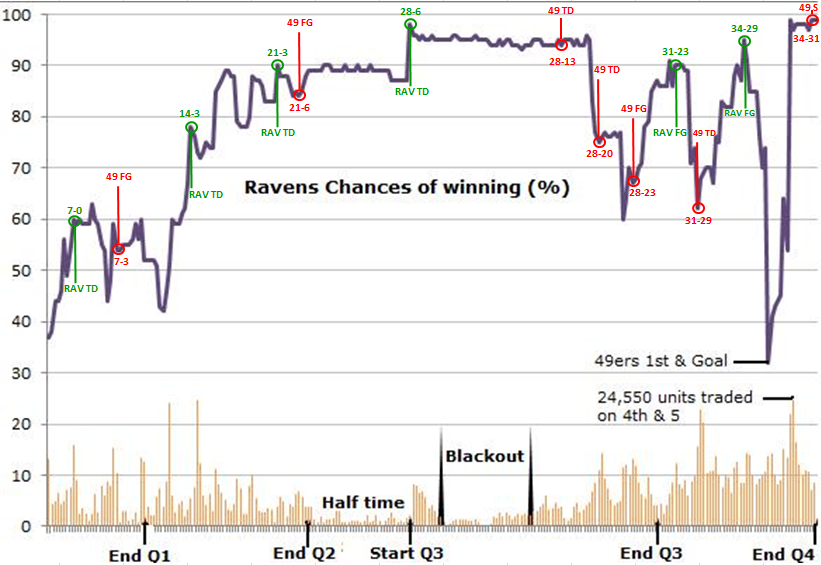
Half Time Analysis
The Ravens took a commanding \(21-6\) lead at half time. Market was trading at \(p_{\frac{1}{2}}^{mkt}= 0.90\).
During the 34 minute blackout 42760 contracts changed hands with Baltimore’s win probability ticking down from 95 to 94.
The win probability peak of 95% occurred after a third-quarter kickoff return for a touchdown.
At the end of the fourth quarter, however, when the 49ers nearly went into the lead with a touchdown, Baltimore’s win probability had dropped to 30%.
Implied Volatility
To calculate the implied volatility of the Superbowl we substitute the pair \((\mu,p) = (-4, .353)\) into our definition and solve for \(\sigma_{IV}\). \[ \sigma = \frac{\mu}{\Phi^{-1}(p)} \, , \]
- We obtain
\[ \sigma_{IV} = \frac{\mu}{\Phi^{-1}(p)} = \frac{-4}{-0.377} = 10.60 \] where \(\Phi^{-1} ( p) = qnorm(0.353) = -0.377\). The 4 point advantage assessed for the 49ers is under a \(\frac{1}{2} \sigma\) favorite.
- The outcome \(X(1)=3\) was within one standard deviation of the pregame model which had an expectation of \(\mu=-4\) and volatility of \(\sigma= 10.6\).
Half Time Probabilities
- What’s the probability of the Ravens winning given their lead at half time?
- At half time Baltimore led by 15 points, 21 to 6.
- The conditional mean for the final outcome is \(15 + 0.5\times(-4) = 13\) and the conditional volatility is \(10.6 \sqrt{1-t}.\)
- These imply a probability of \(.96\) for Baltimore to win the game.
- A second estimate of the probability of winning given the half time lead can be obtained directly from the betting market.
- From the online betting market we also have traded contracts on
TradeSports.comthat yield a half time probability of \(p_{\frac{1}{2}} = 0.90\).
What’s the implied volatility for the second half?
- \(p_t^{mkt}\) reflects all available information
- For example, at half-time \(t = \frac{1}{2}\) we would update
\[ \sigma_{IV,t=\frac{1}{2}} = \frac{ l + \mu ( 1-t ) }{ \Phi^{-1} ( p_t ) \sqrt{1-t}} = \frac{15-2}{ \Phi^{-1}(0.9) / \sqrt{2} } = 14 \] where \(qnorm(0.9)=1.28\).
- As \(14> 10.6\), the market was expecting a more volatile second half–possibly anticipating a comeback from the 49ers.
How can we form a valid betting strategy?
Given the initial implied volatility \(\sigma=10.6\).
At half time with the Ravens having a \(l +\mu(1-t)=13\) points edge
- We would assess with \(\sigma = 10.6\)
\[ p_{\frac{1}{2}} = \Phi \left ( 13/ (10.6/\sqrt{2}) \right ) = 0.96 \] probability of winning versus the \(p_{\frac{1}{2}}^{mkt} = 0.90\) rate.
- To determine our optimal bet size, \(\omega_{bet}\), on the Ravens we might appeal to the Kelly criterion (Kelly, 1956) which yields
\[ \omega_{bet} = p_{\frac{1}{2}} - \frac{q_{\frac{1}{2}}}{O^{mkt}} = 0.96 - \frac{0.1}{1/9} = 0.60 \]
Multivariate Normal
In the multivariate case, the normal-normal model is \[ \theta \sim N(\mu_0,\Sigma_0), \quad y \mid \theta \sim N(\theta,\Sigma). \] The posterior distribution is \[ \theta \mid y \sim N(\mu_1,\Sigma_1), \] where \[ \Sigma_1 = (\Sigma_0^{-1} + \Sigma^{-1})^{-1}, \quad \mu_1 = \Sigma_1(\Sigma_0^{-1}\mu_0 + \Sigma^{-1}y). \] The predictive distribution is \[ y_{new} \mid y \sim N(\mu_1,\Sigma_1 + \Sigma). \]
Black-Litterman
Black and Litterman (1991, 1992) work for combining investor views with market equilibrium.
In a multivariate returns setting the optimal allocation rule is \[ \omega^\star = \frac{1}{\gamma} \Sigma^{-1} \mu \] The question is how to specify \((\mu, \Sigma)\) pairs?
For example, given \(\hat{\Sigma}\), BL derive Bayesian inference for \(\mu\) given market equilibrium model and a priori views on the returns of pre-specified portfolios which take the form \[ ( \hat{\mu} | \mu ) \sim \mathcal{N} \left ( \mu , \tau \hat{\Sigma} \right ) \; {\rm and} \; ( Q | \mu ) \sim \mathcal{N} \left ( P \mu , \hat{\Omega} \right ) \; . \]
Posterior Views
Combining views, the implied posterior is \[ ( \mu | \hat{\mu} , Q ) \sim \mathcal{N} \left ( B b , B \right ) \]
The mean and variance are specified by
\[ B = ( \tau \hat{\Sigma} )^{-1} + P^\prime \hat{\Omega}^{-1} P \; {\rm and} \; b = ( \tau \hat{\Sigma} )^{-1} \hat{\mu} + P^\prime \Omega^{-1} Q \] These posterior moments then define the optimal allocation rule.
Satya Nadella: CEO of Microsoft
- In 2014, Satya Nadella became the CEO of Microsoft.
- The stock price of Microsoft has been on a steady rise since then.
- Suppose that you are a portfolio manager and you are interested in analyzing the returns of Microsoft stock compared to the market.
- Suppose you are managing a portfolio with two positions stock of Microsoft (MSFT) and an index fund that follows S&P500 index and tracks overall market performance.
- What is the mean returns of the positions in our portfolio?
Satya Nadella: CEO of Microsoft
- Assume the prior for the mean returns is a bivariate normal distribution, let \(\mu_0 = (\mu_{M}, \mu_{S})\) represent the prior mean returns for the stocks.
- The covariance matrix \(\Sigma_0\) captures your beliefs about the variability and the relationship between these stocks’ returns in the prior. \[ \Sigma_0 = \begin{bmatrix} \sigma_{M}^2 & \sigma_{MS} \\ \sigma_{MS} & \sigma_{S}^2 \end{bmatrix}, \]
We will use the sample mean and covariance matrix of the historical returns as the prior mean and covariance matrix.
Satya Nadella: CEO of Microsoft
- The likelihood of observing the data, given the mean returns, is also a bivariate normal distribution. \[ \Sigma = \begin{bmatrix} \sigma_{M}^2 & \sigma_{MS} \\ \sigma_{MS} & \sigma_{S}^2 \end{bmatrix}, \] where \(\sigma_{M}^2\) and \(\sigma_{S}^2\) are the sample variances of the observed returns of MSFT and SPY, respectively, and \(\sigma_{MS}\) is the sample covariance of the observed returns of MSFT and SPY. The likelihood mean is given by \[ \mu = \begin{bmatrix} \mu_{M} \\ \mu_{S} \end{bmatrix}, \] where \(\mu_{M}\) and \(\mu_{S}\) are the sample means of the observed returns of MSFT and SPY, respectively.
Satya Nadella: CEO of Microsoft
- You update your beliefs (prior) about the mean returns using the observed data (likelihood).
- The posterior distribution, which combines your prior beliefs and the new information from the data, is also a bivariate normal distribution.
- The mean \(\mu_{\text{post}}\) and covariance \(\Sigma_{\text{post}}\) of the posterior are calculated using Bayesian updating formulas, which involve \(\mu_0\), \(\Sigma_0\), \(\mu\), and \(\Sigma\).
- We use observed returns prior to Nadella’s becoming CEO as our prior and analyze the returns post 2014.
Satya Nadella: CEO of Microsoft
Code
[1] "MSFT" "SPY" Code
s = 3666 # 2015-07-30
prior = 1:s
obs = s:nrow(MSFT) # post covid
# obs = 5476:nrow(MSFT) # 2022-10-06 bull run if 22-23
a = as.numeric(dailyReturn(MSFT))
c = as.numeric(dailyReturn(SPY))
# Prior
mu0 = c(mean(a[prior]), mean(c[prior]))
Sigma0 = cov(data.frame(a=a[prior],c=c[prior]))
# Data
mu = c(mean(a[obs]), mean(c[obs]))
Sigma = cov(data.frame(a=a,c=c))
# Posterior
SigmaPost = solve(solve(Sigma0) + solve(Sigma))
muPost = SigmaPost %*% (solve(Sigma0) %*% mu0 + solve(Sigma) %*% mu)
# Plot
plot(a[obs], c[obs], xlab="MSFT", ylab="SPY", xlim=c(-0.005,0.005), ylim=c(-0.005,0.005), pch=16, cex=0.5)
abline(v=0, h=0, col="grey")
abline(v=mu0[1], h=mu0[2], col="blue",lwd=3) #prior
abline(v=mu[1], h=mu[2], col="red",lwd=3) #data
abline(v=muPost[1], h=muPost[2], col="green",lwd=3) #posterior
legend("bottomright", c("Prior", "Likelihood", "Posterior"), pch=15, col=c("blue", "red", "green"), bty="n")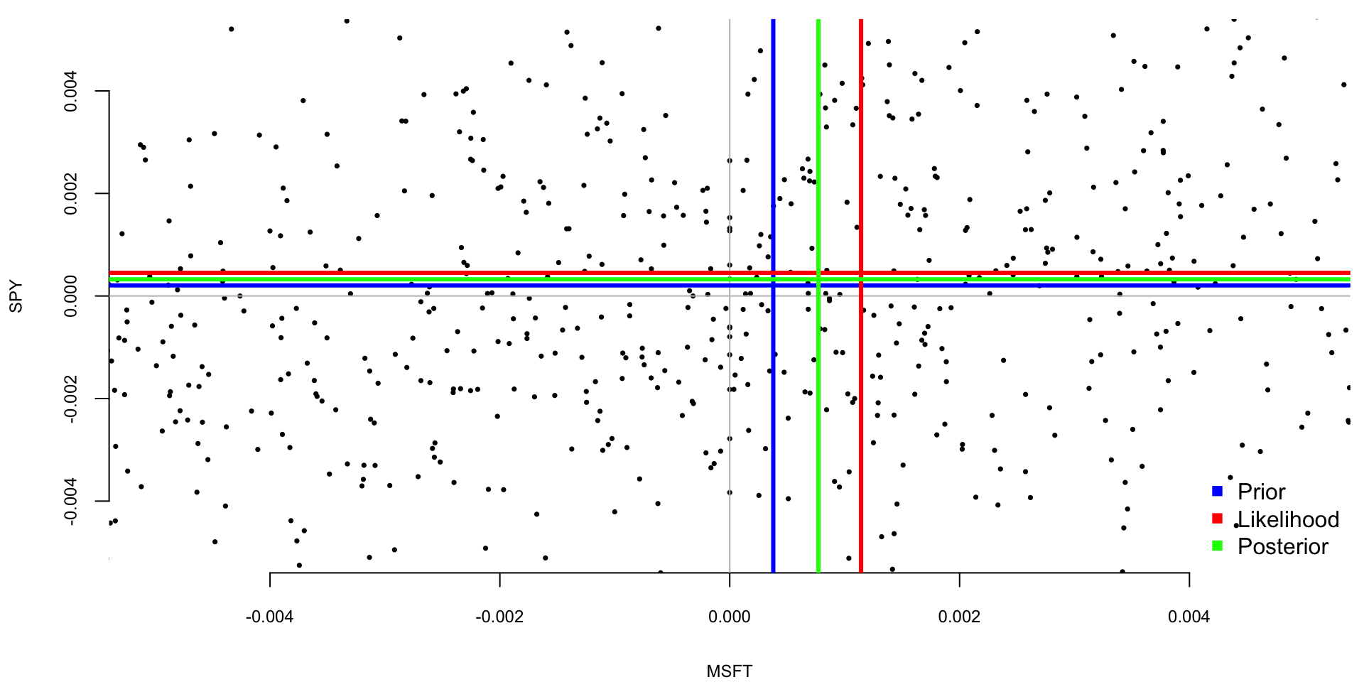
Mixtures of Conjugate Priors
- The mixture of conjugate priors is a powerful tool for modeling complex data. \[ \theta \sim p(\theta) = \sum_{k=1}^K \pi_k p_k(\theta). \] Then the posterior is also a mixture of normal distributions, that is \[ p(\theta\mid y) = p(y\mid \theta)\sum_{k=1}^K \pi_k p_k(\theta)/C. \]
Mixtures of Conjugate Priors
We introduce a normalizing constant for each component \[ C_k = \int p(y\mid \theta)p_k(\theta)d\theta. \] then \[ p_k(\theta\mid y) = p_k(\theta)p(y\mid \theta)/C_k \] is a proper distribution and our posterior is a mixture of these distributions \[ p(\theta\mid y) = \sum_{k=1}^K \pi_k C_k p_k(\theta\mid y)/C. \] Meaning that we need to require \[ \dfrac{\sum_{k=1}^K \pi_k C_k}{C} = 1. \] or \[ C = \sum_{k=1}^K \pi_k C_k \]
Mixture of two normal distributions
The prior distribution is a mixture of two normal distributions, that is \[ \mu \sim 0.5 N(0,1) + 0.5 N(5,1). \] The likelihood is a normal distribution with mean \(\mu\) and variance 1, that is \[ y \mid \mu \sim N(\mu,1). \] The posterior distribution is a mixture of two normal distributions, that is \[ p(\mu \mid y) \propto \phi(y\mid \mu,1) \left(0.5 \phi(\mu\mid 0,1) + 0.5 \phi(\mu\mid 5,1)\right), \] where \(\phi(x\mid \mu,\sigma^2)\) is the normal distribution with mean \(\mu\) and variance \(\sigma^2\).
Mixture of two normal distributions
We can calculate it using property of a normal distribution \[ \phi(x\mid \mu_1,\sigma_1^2)\phi(x\mid \mu_2,\sigma_2^2) = \phi(x\mid \mu_3,\sigma_3^2)\phi(\mu_1-\mu_2\mid 0,\sigma_1^2+\sigma_2^2) \] where \[ \mu_3 = \dfrac{\mu_1/\sigma_2^2 + \mu_2/\sigma_1^2}{1/\sigma_1^2 + 1/\sigma_2^2}, \quad \sigma_3^2 = \dfrac{1}{1/\sigma_1^2 + 1/\sigma_2^2}. \]
Mixture of two normal distributions
Given, we observed \(y = 2\), we can calculate the posterior distribution for \(\mu\)
Code
mu0 = c(0,5)
sigma02 = c(1,1)
pi = c(0.5,0.5)
y = 2
mu3 = (mu0/sigma02 + y) / (1/sigma02 + 1)
sigma3 = 1/(1/sigma02 + 1)
C = dnorm(y-mu0,0,1+sigma02)*pi
w = C/sum(C)
cat(sprintf("Component parameters:\nMean = (%1.1f,%2.1f)\nVar = (%1.1f,%1.1f)\nweights = (%1.2f,%1.2f)", mu3[1],mu3[2], sigma3[1],sigma3[2],w[1],w[2]))
Component parameters:
Mean = (1.0,3.5)
Var = (0.5,0.5)
weights = (0.65,0.35)Normal With Unknown Variance
Consider, another example, when mean \(\mu\) is fixed and variance is a random variable which follows some distribution \(\sigma^2 \sim p(\sigma^2)\). Given an observed sample \(y\), we can update the distribution over variance using the Bayes rule \[ p(\sigma^2 \mid y) = \dfrac{p(y\mid \sigma^2 )p(\sigma^2)}{p(y)}. \] Now, the total probability in the denominator can be calculated as \[ p(y) = \int p(y\mid \sigma^2 )p(\sigma^2) d\sigma^2. \]
Normal With Unknown Variance
A conjugate prior that leads to analytically calculable integral for variance under the normal likelihood is the inverse Gamma. Thus, if \[ \sigma^2 \mid \alpha,\beta \sim IG(\alpha,\beta) = \dfrac{\beta^{\alpha}}{\Gamma(\alpha)}\sigma^{2(-\alpha-1)}\exp\left(-\dfrac{\beta}{\sigma^2}\right) \] and \[ y \mid \mu,\sigma^2 \sim N(\mu,\sigma^2) \] Then the posterior distribution is another inverse Gamma \(IG(\alpha_{\mathrm{posterior}},\beta_{\mathrm{posterior}})\), with \[ \alpha_{\mathrm{posterior}} = \alpha + 1/2, ~~\beta_{\mathrm{posterior}} = \beta + \dfrac{y-\mu}{2}. \]
Normal With Unknown Variance
Now, the predictive distribution over \(y\) can be calculated by \[ p(y_{new}\mid y) = \int p(y_{new},\sigma^2\mid y)p(\sigma^2\mid y)d\sigma^2. \] Which happens to be a \(t\)-distribution with \(2\alpha_{\mathrm{posterior}}\) degrees of freedom, mean \(\mu\) and variance \(\alpha_{\mathrm{posterior}}/\beta_{\mathrm{posterior}}\).
The Normal-Gamma Model
- To simplify the formulas, we use precision \(\rho = 1/\sigma^2\) instead of variance \(\sigma^2\). The normal-Gamma distribution is a conjugate prior for the normal distribution, when we do not know the precision and the mean. Given the observed data \(Y = \{y_1,\ldots,y_n\}\), we assume normal likelihood \[ y_i \mid \theta, \rho \sim N(\theta, 1/\rho) \]
The normal-gamma prior distribution is defined as \[ \theta\mid \mu,\rho,\nu \sim N(\mu, 1/(\rho \nu)), \quad \rho \mid \alpha, \beta \sim \text{Gamma}(\alpha, \beta). \] - \(1/\rho\) has inverse-Gamma distribution with parameters \(\alpha\) and \(\beta\). - Conditional on \(\rho\), the mean \(\theta\) has normal distribution with mean \(\mu\) and precision \(\nu\rho\).
The Normal-Gamma Model
\[ \theta\mid \mu,\rho,\nu \sim N(\mu, 1/(\rho \nu)), \quad \rho \mid \alpha, \beta \sim \text{Gamma}(\alpha, \beta). \]
- The mean \(\theta\) and precision \(\rho\) are not independent.
- When the precision of observations \(\rho\) is low, we are also less certain about the mean.
- When \(\nu=0\), we have an improper uniform distribution over \(\theta\), that is independent of \(\rho\).
- There is no conjugate distribution for \(\theta,\rho\) in which \(\theta\) is independent of \(\rho\).
The Normal-Gamma Model
Given the normal likelihood \[ p(y\mid \theta, \rho) = \left(\dfrac{\rho}{2\pi}\right)^{1/2}\exp\left(-\dfrac{\rho}{2}\sum_{i=1}^n(y_i-\theta)^2\right) \] and the normal-gamma prior \[ p(\theta, \rho \mid \mu,\nu,\alpha,\beta) = \dfrac{\beta^\alpha}{\Gamma(\alpha)}\nu\rho^{\alpha-1}\exp(-\beta\rho)\left(\dfrac{\nu\rho}{2\pi}\right)^{1/2}\exp\left(-\dfrac{\nu\rho}{2}(\theta-\mu)^2\right) \] the posterior distribution is given by \[ p(\theta, \rho\mid y) \propto p(y\mid \theta, \rho)p(\theta, \rho). \] The posterior distribution is a normal-Gamma distribution with parameters \[ \begin{aligned} \mu_n &= \dfrac{\nu\mu + n\bar{y}}{\nu+n},\\ \nu_n &= \nu+n,\\ \alpha_n &= \alpha + \dfrac{n}{2},\\ \beta_n &= \beta + \dfrac{1}{2}\sum_{i=1}^n(y_i-\bar{y})^2 + \dfrac{n\nu}{2(\nu+n)}(\bar{y}-\mu)^2. \end{aligned} \]
The Normal-Gamma Model
- \(\bar{y} = n^{-1}\sum_{i=1}^n y_i\) is the sample mean and \(n\) is the sample size.
- The posterior distribution is a normal-Gamma distribution with parameters \(\mu_n, \nu_n, \alpha_n, \beta_n\).
Credible Intervals for Normal-Gamma Model Posterior Parameters
- The precission posterior follows a Gamma distribution with parameters \(\alpha_n, \beta_n\), thus we can use quantiles of the Gamma distribution to calculate credible intervals.
- A symmetric \(100(1-c)%\) credible interval \([g_{c/2},g_{1-c/2}]\) is given by \(c/2\) and \(1-c/2\) quantiles of the gamma distrinution. To find credible intterval for the variance \(v = 1/\rho\), we simply use \[ [1/g_{1-c/2},1/g_{c/2}]. \] and for standard deviation \(s = \sqrt{v}\) we use \[ [\sqrt{1/g_{1-c/2}},\sqrt{1/g_{c/2}}]. \]
To find credible interval over the mean \(\theta\), we need to integrate out the precision \(\rho\) from the posterior distribution. The marginal distribution of \(\theta\) is a Student’s t-distribution with parameters center at \(\mu_n\), variance \(\beta_n/(\nu_n\alpha_n)\) and degrees of freedom \(2\alpha_n\).
Exponential-Gamma Model
- Waiting times between events: consecutive arrivals of a Poisson process is exponentially distributed with mean \(1/\lambda\). \[ f(x;\lambda) = \lambda e^{-\lambda x}, ~ x \geq 0 \]
- \(\lambda\) is the rate parameter, which is the inverse of the mean
- special case of the Gamma distribution with shape 1 and scale \(1/\lambda\).
| Exponential Distribution | Parameters |
|---|---|
| Expected value | \(\mu = E{X} = 1/\lambda\) |
| Variance | \(\sigma^2 = Var{X} = 1/\lambda^2\) |
Exponential Model: Examples
- Lifespan of Electronic Components: The exponential distribution can model the time until a component fails in systems where the failure rate is constant over time.
- Time Between Arrivals: In a process where events (like customers arriving at a store or calls arriving at a call center) occur continuously and independently, the time between these events can often be modeled with an exponential distribution.
- Radioactive Decay: The time until a radioactive atom decays is often modeled with an exponential distribution.
Exponential-Gamma Model
The Exponential-Gamma model assumes that the data follows an exponential distribution (likelihood). - The Gamma distribution is a flexible two-parameter family of distributions and can model a wide range of shapes. \[\begin{align*} \lambda &\sim \text{Gamma}(\alpha, \beta) \\ x_i &\sim \text{Exponential}(\lambda) \end{align*}\]
The posterior distribution of the rate parameter \(\lambda\) is given by: \[ p(\lambda\mid x_1, \ldots, x_n) \propto \lambda^{\alpha - 1} e^{-\beta\lambda} \prod_{i=1}^n \lambda e^{-\lambda x_i} = \lambda^{\alpha + n - 1} e^{-(\beta + \sum_{i=1}^n x_i)\lambda} \]
Exponential-Gamma Model
Posterior is a Gamma distribution with shape parameter \(\alpha + n\) and rate parameter \(\beta + \sum_{i=1}^n x_i\). The posterior mean and variance are given by: \[ \mathbb{E}[\lambda|x_1, \ldots, x_n] = \frac{\alpha + n}{\beta + \sum_{i=1}^n x_i}, \quad \mathrm{Var}[\lambda|x_1, \ldots, x_n] = \frac{\alpha + n}{(\beta + \sum_{i=1}^n x_i)^2}. \] Notice, that \(\sum x_i\) is the sufficient statistic for inference about parameter \(\lambda\)!
Exponential-Gamma Model
- Reliability Engineering: In situations where the failure rate of components or systems may not be constant and can vary, the Exponential-Gamma model can be used to estimate the time until failure, incorporating uncertainty in the failure rate.
- Medical Research: For modeling survival times of patients where the rate of mortality or disease progression is not constant and varies across a population. The variability in rates can be due to different factors like age, genetics, or environmental influences.
- Ecology: In studying phenomena like the time between rare environmental events (e.g., extreme weather events), where the frequency of occurrence can vary due to changing climate conditions or other factors.
Exploratory Data Analysis
Before deciding on a parametric model for a dataset. There are several tools that we use to choose the appropriate model. These include
- Theoretical assumptions underlying the distribution (our prior knowledge about the data)
- Exploratory data analysis
- Formal goodness-of-fit tests
The two most common tools for exploratory data analysis are Q-Q plot, scatter plots and bar plots/histograms.
Q-Q plot
- Q-Q plot simply compares the quantiles of your data with the quantiles of a theoretical distribution (like normal, exponential, etc.).
- Quantile is the fraction (or percent) of points below the given value.
- That is, the \(i\)-th quantile is the point \(x\) for which \(i\)% of the data lies below \(x\).
- On a Q-Q plot, if the two data sets come from a population with the same distribution, we should see the points forming a line that’s roughly straight.
Q-Q plot
- If the two data sets \(x\) and \(y\) come from the same distribution, then the points \((x_{(i)}, y_{(i)})\) should lie roughly on the line \(y = x\).
- If \(y\) comes from a distribution that’s linear in \(x\), then the points \((x_{(i)}, y_{(i)})\) should lie roughly on a line, but not necessarily on the line \(y = x\).
Noraml Q-Q plot
Q-Q plot for the Data on birth weights of babies born in a Brisbane hospital on December 18, 1997. The data set contains 44 records. A more detailed description of the data set can be found in UsingR manual.
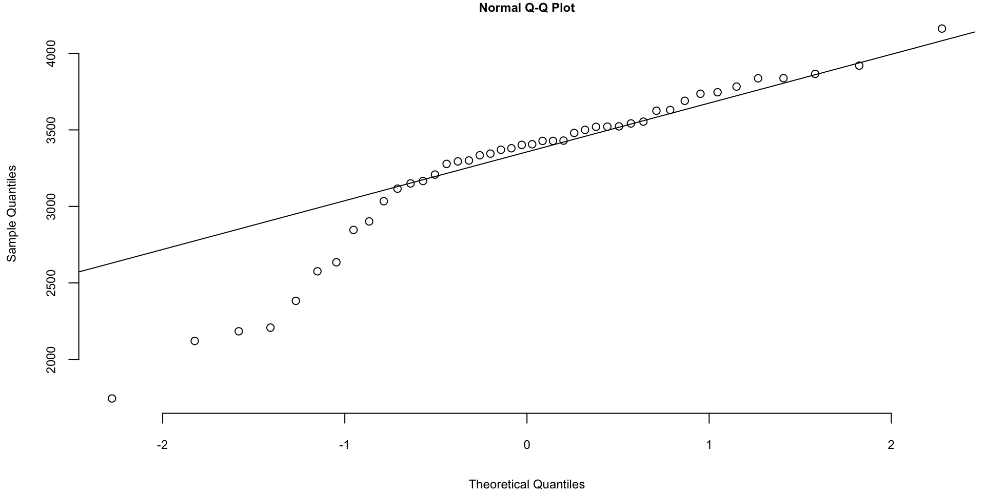
Figure 1
Are Birth Weights Normally Distributed?
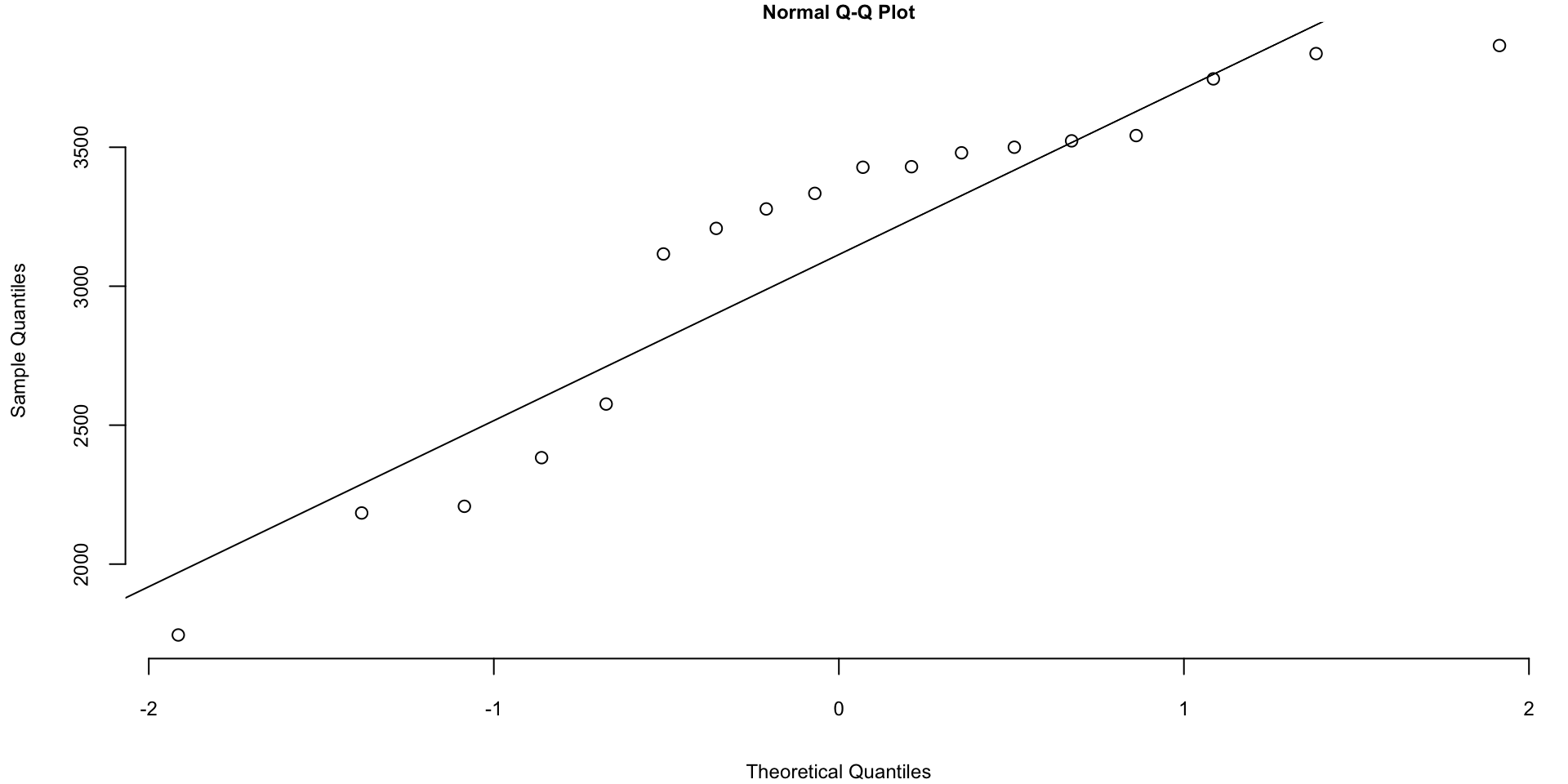
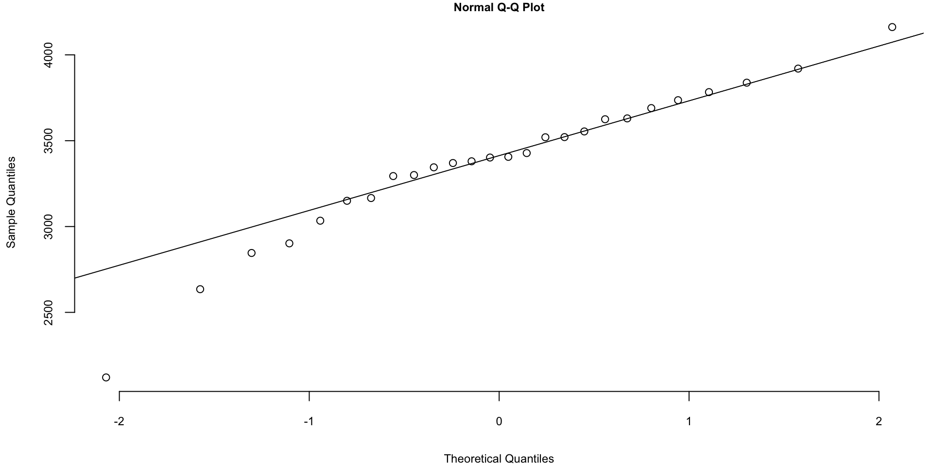
Noraml Q-Q plot
The Q-Q plots look different if we split the data based on the gender
Code
Histogram of baby weights by gender
Noraml Q-Q plot
How about the times in hours between births of babies?
Code
hr = ceiling(babyboom$running.time/60)
BirthsByHour = tabulate(hr)
# Number of hours with 0, 1, 2, 3, 4 births
ObservedCounts = table(BirthsByHour)
# Average number of births per hour
BirthRate=sum(BirthsByHour)/24
# Expected counts for Poisson distribution
ExpectedCounts=dpois(0:4,BirthRate)*24
# bind into matrix for plotting
ObsExp <- rbind(ObservedCounts,ExpectedCounts)
barplot(ObsExp,names=0:4, beside=TRUE,legend=c("Observed","Expected"))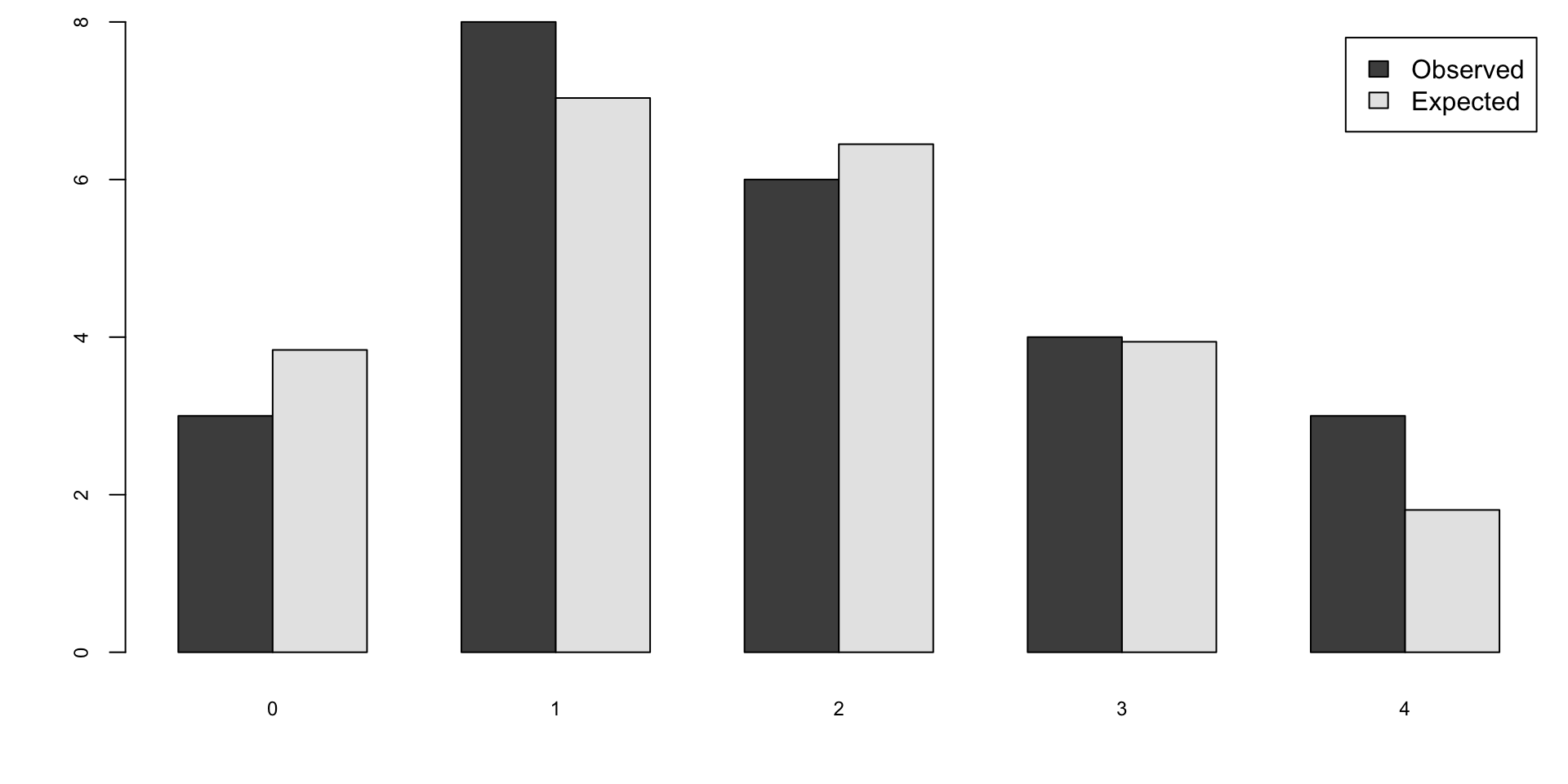
Exponential Q-Q plot
What about the Q-Q plot?
Code
# birth intervals
birthinterval=diff(babyboom$running.time)
 # quantiles of standard exponential distribution (rate=1)
exponential.quantiles = qexp(ppoints(43))
qqplot(exponential.quantiles, birthinterval)
lmb=mean(birthinterval)
lines(exponential.quantiles,exponential.quantiles*lmb) # Overlay a line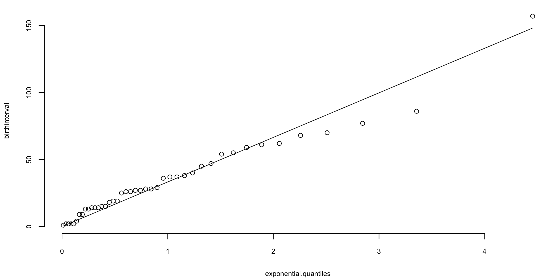
Here
ppointsfunction computes the sequence of probability pointsqexpfunction computes the quantiles of the exponential distributiondifffunction computes the difference between consecutive elements of a vector
Brief List of Conjugate Models
| Likelihood | Prior | Posterior |
|---|---|---|
| Binomial | Beta | Beta |
| Negative | Binomial | Beta |
| Poisson | Gamma | Gamma |
| Geometric | Beta | Beta |
| Exponential | Gamma | Gamma |
| Normal (mean unknown) | Normal | Normal |
| Normal (variance unknown) | Inverse Gamma | Inverse Gamma |
| Normal (mean and variance unknown) | Normal/Gamma | Normal/Gamma |
| Multinomial | Dirichlet | Dirichlet |