Bayes AI
Unit 4: Bayesian Hypothesis Tests

Vadim Sokolov
George Mason University
Spring 2025
Bayesian Hypothesis Testing
- Given sample of data, \(y\), generated from \(p\left( y \mid \theta\right)\) for \(\theta\in\Theta\)
- Determine if \(\theta\) lies in \(\Theta_{0}\) or in \(\Theta_{1}\)
- Two disjoint subsets of \(\Theta\). In general, the hypothesis testing problem involves an action: accepting or rejecting a hypothesis.
- A null, \(H_{0}\), and alternative hypothesis, \(H_{1}\), which are defined as \[ H_{0}:\theta\in\Theta_{0}\;\;\mathrm{and}\;\;H_{1}% :\theta\in\Theta_{1}\text{.}% \]
Bayesian Hypothesis Testing
- \(\Theta _{0}=\theta_{0}\): simple or “sharp” null hypothesis.
- Composite, otherwise
- Single parameter: typical one-sided tests are of the form \(H_{0}:\theta<\theta_{0}\) and \(H_{1}:\theta>\theta_{0}\).
| \(\theta\in\Theta_{0}\) | \(\theta\in\Theta_{1}\) | |
|---|---|---|
| Accept \(H_{0}\) | Correct decision | Type II error |
| Accept \(H_{1}\) | Type I error | Correct decision |
Bayesian Hypothesis Testing: Errors
Formally, the probabilities of Type I (\(\alpha\)) and Type II (\(\beta\)) errors are defined as: \[ \alpha=P \left[ \text{reject }H_{0} \mid H_{0}\text{ is true }\right] \text{ and }\beta=P \left[ \text{accept }H_{0} \mid H_{1}\text{ is true }\right] \text{.}% \]
- It is useful to think of the decision to accept or reject as a decision rule, \(d\left( y\right)\).
- In many cases, the decision rules form a critical region \(R\), such that \(d\left( y\right) =d_{1}\) if \(y\in R\).
- These regions are often take the form of simple inequalities.
\[\begin{align*} \alpha_{\theta}\left( d\right) & =P \left[ d\left( y\right) =d_{1} \mid \theta\right] \text{ if }\theta\in\Theta_{0}\text{ }(H_{0}\text{ is true})\\ \beta_{\theta}\left( d\right) & =P \left[ d\left( y\right) =d_{0} \mid \theta\right] \text{ if }\theta\in\Theta_{1}\text{ }(H_{1}\text{ is true})\text{.}% \end{align*}\] Errors explicitly depend on the decision and the true parameter value
Bayesian Hypothesis Testing
- The size of the test (the probability of making a type I error) is defined as \[ \alpha = \underset{\theta\in\Theta_{0}}{\sup}~\alpha_{\theta}\left( d\right) \]
- The power is defined as \(1-\beta_{\theta}\left( d\right)\).
- It is always possible to set either \(\alpha_{\theta}\left( d\right)\) or \(\beta_{\theta }\left( d\right)\) equal to zero, by finding a test that always rejects alternative or null, respectively.
- The total probability of making an error is \(\alpha_{\theta}\left(d\right) +\beta_{\theta}\left(d\right)\), want to minimize
Bayesian Hypothesis Testing
- The optimal action \(d^*\) minimizes the posterior expected loss, is \(d^* = d_0 = 0\) if the posterior probability of hypothesis \(H_0\) exceeds 1/2, and \(d^* = d_1=1\) else \[ d^* = 1\left( P \left( \theta \in \Theta_0 \mid y\right) < P \left( \theta \in \Theta_1 \mid y\right)\right) = 1\left(P \left( \theta \in \Theta_0 \mid y\right)<1/2\right). \]
- Simply speaking, the hypothesis with higher posterior probability is selected.
- More data reduces the error probability
- Sometimes we can derive optimal tests, those that minimize the sum of the errors.
Bayesian Hypothesis Testing
- Simple hypothesis tests \(H_{0}:\theta=\theta_{0}\) versus \(H_{1}:\theta=\theta_{1}\) admit optimal tests
- Defining \(d^{\ast}\) as a test accepting \(H_{0}\) if \(a_{0}f\left( y \mid \theta_{0}\right) >a_{1}f\left( y \mid \theta_{1}\right)\) and \(H_{1}\) if \(a_{0}f\left( y \mid \theta_{0}\right) <a_{1}f\left( y \mid \theta _{1}\right)\), for some \(a_{0}\) and \(a_{1}\).
- Either \(H_{0}\) or \(H_{1}\) can be accepted if \(a_{0}f\left(y \mid \theta_{0}\right) =a_{1}f\left( y \mid \theta_{1}\right)\). Then, for any other test \(d\), it is not hard to show that \[ a_{0}\alpha\left( d^{\ast}\right) +a_{1}\beta\left( d^{\ast}\right) \leq a_{0}\alpha\left( d\right) +a_{1}\beta\left( d\right), \] where \(\alpha_{d}=\alpha_{d}\left( \theta\right)\) and \(\beta_{d}=\beta_{d}\left( \theta\right)\).
Bayesian Hypothesis Testing
- This result highlights the optimality of tests defining rejection regions in terms of the likelihood ratio statistic, \(f\left( y \mid \theta_{0}\right)/f\left( y \mid \theta_{1}\right)\).
- It turns out that the results are in fact stronger.
- In terms of decision theoretic properties, tests that define rejection regions based on likelihood ratios are not only admissible decisions, but form a minimal complete class, the strongest property possible.
Bayesian Hypothesis Testing
- Tradeoff between the two goals of reducing type I and type II errors: decreasing \(\alpha\) leads to an increase in \(\beta\), and vice-versa.
- It is common to fix \(\alpha_{\theta}\left( d\right)\), or \(\sup~\alpha_{\theta}\left( d\right)\), and then find a test to minimize \(\beta_{d}\left( \theta\right)\).
- This leads to “most powerful” tests.
- Important result from decision theory: test procedures that use the same size level of \(\alpha\) in problems with different sample sizes are inadmissible.
- This is commonly done where significance is indicated by a fixed size, say 5%. The implications of this will be clearer below in examples.
Testing fairness
Suppose we are interested in testing \(\theta\), the unknown probability of heads for possibly biased coin. Suppose, \[ H_0 :~\theta=1/2 \quad\text{v.s.} \quad H_1 :~\theta>1/2. \] An experiment is conducted and 9 heads and 3 tails are observed. This information is not sufficient to fully specify the model \(p(y\mid \theta)\). There are two approaches.
Testing fairness
Scenario 1: Number of flips, \(n = 12\) is predetermined. Then number of heads \(Y \mid \theta\) is binomial \(B(n, \theta)\), with probability mass function \[ p(y\mid \theta)= {n \choose x} \theta^x(1−\theta)^{n−x} = 220 \cdot \theta^9(1−\theta)^3 \] For a frequentist, the p-value of the test is \[ P(Y \geq 9\mid H_0)=\sum_{y=9}^{12} {12 \choose y} (1/2)^y(1−1/2)^{12−y} = (1+12+66+220)/2^{12} =0.073, \] and if you recall the classical testing, the \(H_0\) is not rejected at level \(\alpha = 0.05\).
Testing fairness
Scenario 2: Number of tails (successes) \(\alpha = 3\) is predetermined, i.e, the flipping is continued until 3 tails are observed. Then, \(Y\) - number of heads (failures) until 3 tails appear is Negative Binomial \(NB(3, 1− \theta)\), \[ p(y\mid \theta)= {\alpha+y-1 \choose \alpha-1} \theta^{y}(1−\theta)^{\alpha} = {3+9-1 \choose 3-1} \theta^9(1−\theta)^3 = 55\cdot \theta^9(1−\theta)^3. \] For a frequentist, large values of \(Y\) are critical and the p-value of the test is \[ P(Y \geq 9\mid H_0)=\sum_{y=9}^{\infty} {3+y-1 \choose 2} (1/2)^{x}(1/2)^{3} = 0.0327. \] We used the following identity here \[ \sum_{x=k}^{\infty} {2+x \choose 2}\dfrac{1}{2^x} = \dfrac{8+5k+k^2}{2^k}. \] The hypothesis \(H_0\) is rejected, and this change in decision is not caused by observations.
This is the violation of the likelihoood principle.
The Bayesian Approach
Compute the posterior distribution of each hypothesis \(H_i: \theta \in \Theta_i, ~ i=0,1\). By Bayes rule \[ P \left( H_{i} \mid y\right) =\frac{p\left( y \mid H_{i}\right) P \left( H_{i}\right) }{p\left( y\right)} \] where \(P \left( H_{i}\right)\) is the prior probability of \(H_{i}\), \[ p\left( y \mid H_{i}\right) =\int_{\theta \in \Theta_i} p\left( y \mid \ \theta\right) p\left( \theta \mid H_{i}\right) d\theta \] is the marginal likelihood under \(H_{i}\), \(p\left( \theta \mid H_{i}\right)\) is the parameter prior under \(H_{i}\), and \[ p(y) = p\left(y \mid H_0\right)P(H_0) + p\left(y \mid H_1\right)P(H_1) \]
The Bayesian Approach
If the hypothesis are mutually exclusive, \(P \left( H_{0}\right) =1-P \left( H_{1}\right)\). \[ \text{Odds}_{0,1}=\frac{P \left( H_{0} \mid y\right) }{P % \left( H_{1} \mid y\right) }=\frac{p\left( y \mid H_{0}\right) }{p\left( y \mid H_{1}\right) }\frac{P \left( H_{0}\right) }{P \left( H_{1}\right) }\text{.}% \]
The odds ratio updates the prior odds, \(P \left( H_{0}\right) /P \left( H_{1}\right)\), using the Bayes Factor, \[ \mathcal{BF}_{0,1}=\dfrac{p\left(y \mid H_{0}\right)}{p\left( y \mid H_{1}\right)}. \] With exhaustive competing hypotheses\(,\) \(P \left( H_{0} \mid y\right)\) simplifies to \[ P \left( H_{0} \mid y\right) =\left( 1+\left( \mathcal{BF}_{0,1}\right) ^{-1}\frac{\left( 1-P \left( H_{0}\right) \right) }{P \left( H_{0}\right) }\right) ^{-1}\text{,}% \] and with equal prior probability, \[ p\left( H_{0} \mid y\right) =\left( 1+\left( \mathcal{BF}_{0,1}\right) ^{-1}\right) ^{-1} \]
Jeffreys’ Scale
For \(\mathcal{BF}_{0,1}>1\)
| \(\mathcal{BF}_{0,1}\) | \(log10(\mathcal{BF}_{0,1})\) | Grades of evidence |
|---|---|---|
| \(1\) to \(10^{1/2}\) | 0 to 1/2 | Barely worth mentioning |
| \(10^{1/2}\) to \(10\) | 1/2 to 1 | Substantial |
| \(10\) to \(10^{3/2}\) | 1 to 3/2 | Strong |
| \(10^{3/2}\) to \(10^{2}\) | 3/2 to 2 | Very strong |
| > \(10^{2}\) | > 2 | Decisive |
Jeffreys’ Scale
For \(\mathcal{BF}_{0,1}<1\)
| \(\mathcal{BF}_{0,1}\) | \(log10(\mathcal{BF}_{0,1})\) | Grades of evidence |
|---|---|---|
| \(1\) to \(10^{-1/2}\) | 0 to -1/2 | Barely worth mentioning |
| \(10^{-1/2}\) to \(10^{-1}\) | -1/2 to -1 | Substantial |
| \(10^{-1}\) to \(10^{-3/2}\) | -1 to -3/2 | Strong |
| \(10^{-3/2}\) to \(10^{-2}\) | -3/2 to -2 | Very strong |
| < \(10^{-2}\) | < -2 | Decisive |
How to make a decision
- The loss incurred when accepting the null (alternative) when the alternative is true (false) is \(L\left( d_{0} \mid H_{1}\right)\) and \(L\left( d_{1} \mid H_{0}\right)\), respectively.
- Assumes a zero loss of making a correct decision
- The Bayesian will accept or reject based on the posterior expected loss \[ \mathbb{E}\left[ \text{Loss}\mid d_{0},y\right] =L\left( d_{0} \mid H_{0}\right) P \left( H_{0} \mid y\right) +L\left( d_{0} \mid H_{1}\right) P \left( H_{1} \mid y\right) =L\left( d_{0} \mid H_{1}\right) P \left( H_{1} \mid y\right) , \] vs \[ \mathbb{E}\left[ \text{Loss} \mid d_{1},y\right] =L\left( d_{1} \mid H_{0}\right) P \left( H_{0} \mid y\right) +L\left( d_{1} \mid H_{1}\right) P \left( H_{1} \mid y\right) =L\left( d_{1} \mid H_{0}\right) P \left( H_{0} \mid y\right) . \]
How to make a decision
\[ \frac{L\left( d_{0} \mid H_{1}\right) }{L\left( d_{1} \mid H_{0}\right) }<\frac{P \left( H_{0} \mid y\right) }{P \left( H_{1} \mid y\right) }. \] In the case of equal prior probabilities, this reduces to \[ \frac{L\left( d_{0} \mid H_{1}\right) }{L\left( d_{1} \mid H_{0}\right) }<\frac{1}{\mathcal{BF}_{0,1}}. \]
Signal Transmission Example
- Random variable \(X\) is transmitted over a noisy communication channel. Assume that the received signal is given by \[ Y=X+W, \] where \(W\sim N(0,\sigma^2)\) is independent of \(X\).
- Suppose that \(X=1\) with probability \(p\), and \(X=−1\) with probability \(1−p\).
- The goal is to decide between \(X=1\) and \(X=−1\) by observing the random variable \(Y\). We will assume symmetric loss and will accept the hypothesis with the higher posterior probability. This is also sometimes called the maximum a posteriori (MAP) test.
Signal Transmission Example
We assume that \(H_0: ~ X = 1\), thus \(Y\mid X_0 \sim N(1,\sigma^2)\), and \(Y\mid X_1 \sim N(-1,\sigma^2)\). The Bayes factor is simply the likelihood ratio \[ \dfrac{p(y\mid H_0)}{p(y \mid H_1)} = \exp\left( \frac{2y}{\sigma^2}\right). \] The propr odds are \(p/(1-p)\), thus the posterior odds are \[ \exp\left( \frac{2y}{\sigma^2}\right)\dfrac{p}{1-p}. \] We choose \(H_0\) (true \(X\) is 1), if the posterior odds are greater than 1, i.e., \[ y > \frac{\sigma^2}{2} \log\left( \frac{p}{1-p}\right) = c. \]
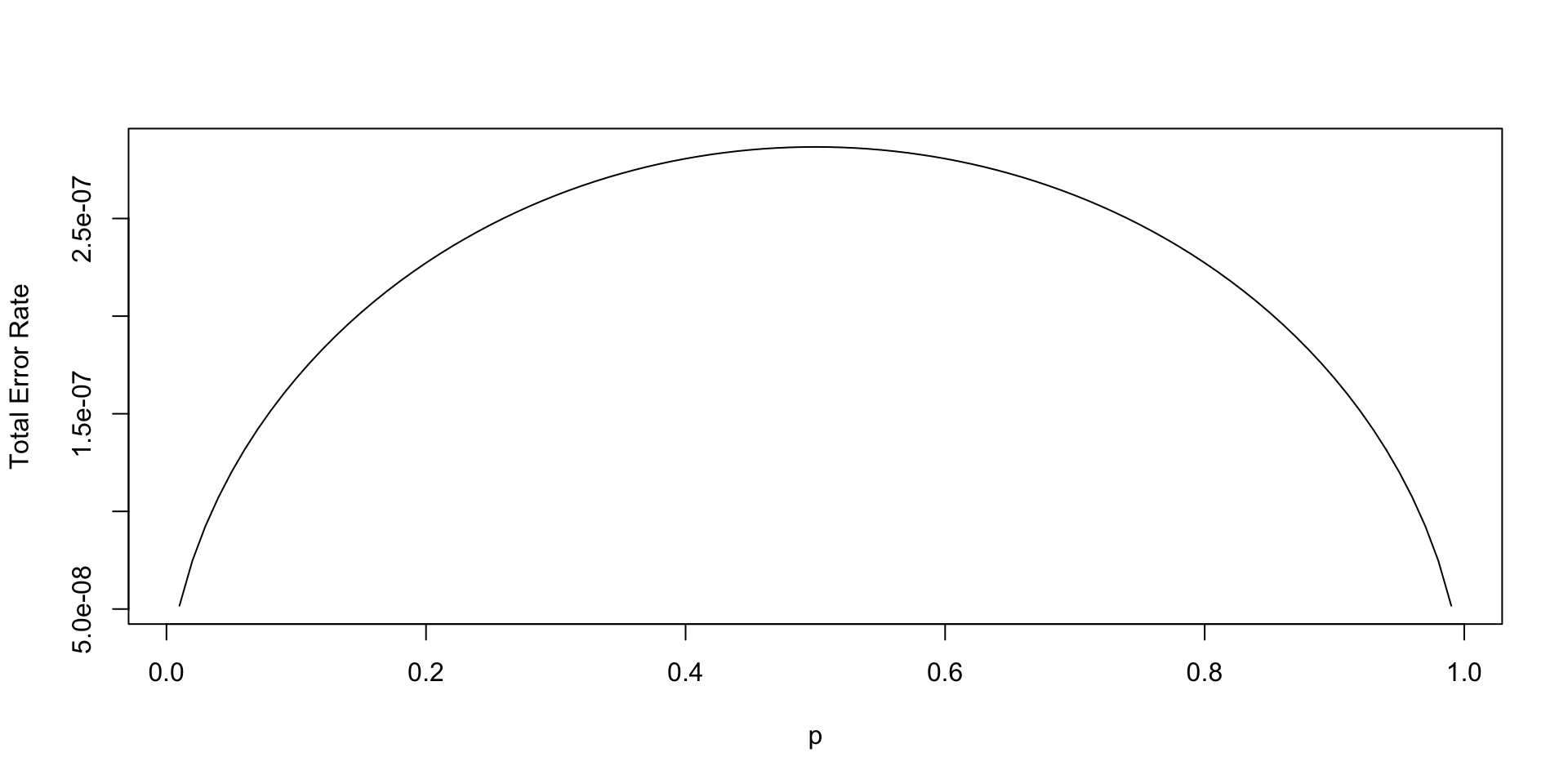
Signal Transmission Example
Further, we can calculate the error probabilities of our test. \[ p(d_1\mid H_0) = P(Y<c\mid X=1) = \Phi\left( \frac{c-1}{\sigma}\right), \] and \[ p(d_0\mid H_1) = P(Y>c\mid X=-1) = 1- \Phi\left( \frac{c+1}{\sigma}\right). \] Let’s plot the total error rate as a function of \(p\) and assuming \(\sigma=0.2\) \[ P_e = p(d_1\mid H_0) (1-p) + p(d_0\mid H_1) p \]
Signal Transmission Example
Hockey: Hypothesis Testing for Normal Mean
- General manager of Washington Capitals (an NHL hockey team) thinks that their star center player Evgeny Kuznetsov is underperformed and is thinking of trading him to a different team.
- He uses the number of goals per season as a metric of performance.
- Prior: a top forward scores on average 30 goals per season with a standard deviation of 5, \(\theta \sim N(30,25)\).
- Data: In the 2022-2023 season Kuznetsov scored 12 goals and likelihood \(X\mid \theta \sim N(\theta, 36)\).
- Kuznetsov’s performance was not stable over the years, thus high variance in the likelihood. Thus, the posterior is \(N(23,15)\).
Hockey
- The manager thinks, that Kuznetsov simply had a bad year and his true performance is at least 24 goals per season \[ H_0: \theta > 24$, ~H_1: \theta<24 \] The posterior probability of \(H_0\) hypothesis is
It is less than 1/2, only 36%. Thus, we should reject the null hypothesis. The posterior odds in favor of the null hypothesis is
Add Loss
- If underestimating (and trading) Kuznetsov is two times more costly than overestimating him (fans will be upset and team spirit might be affected) \[ L(d_1\mid H_0) = 2L(d_0\mid H_1) \]
- Then we should accept the null when posterior odds are greater than 1/2.
The posterior odds are in favor of the null hypothesis. Thus, the manager should not trade Kuznetsov.
Kuznetsov was traded to Carolina Hurricanes towards the end of the 2023-2024 season.
Two-Sided Test for Normal Mean
\(H_0: \theta = m_0\), \(p\left( \theta \mid H_{0}\right) =\delta_{m_{0}}\left( \theta\right)\)
\(H_1: \theta \neq m_0\), \(p\left( \theta \mid H_{1}\right) = N\left( m_{0},\sigma^{2}/n_0\right)\)
Where \(n\) is the sample size and \(\sigma^2\) is the variance (known) of the population. Observed samples are \(Y = (y_1, y_2, \ldots, y_n)\) with \[ y_i \sim N(\theta, \sigma^2). \]
Bayes Factor
The Bayes factor can be calculated analytically \[ BF_{0,1} = \frac{p(Y\mid \theta = m_0, \sigma^2 )} {\int p(Y\mid \theta, \sigma^2) p(\theta \mid m_0, n_0, \sigma^2)\, d \theta} \] \[ \int p(Y\mid \theta, \sigma^2) p(\theta \mid m_0, n_0, \sigma^2)\, d \theta = \frac{\sqrt{n_0}\exp\left\{-\frac{n_0(m_0-\bar y)^2}{2\left(n_0+n\right)\sigma^2}\right\}}{\sqrt{2\pi}\sigma^2\sqrt{\frac{n_0+n}{\sigma^2}}} \] \[ p(Y\mid \theta = m_0, \sigma^2 ) = \frac{\exp\left\{-\frac{(\bar y-m_0)^2}{2 \sigma ^2}\right\}}{\sqrt{2 \pi } \sigma } \]
Bayes Factor
Thus, the Bayes factor is \[ BF_{0,1} = \frac{\sigma\sqrt{\frac{n_0+n}{\sigma^2}}e^{-\frac{(m_0-\bar y)^2}{2\left(n_0+n\right)\sigma^2}}}{\sqrt{n_0}} \]
\[ BF_{0,1} =\left(\frac{n + n_0}{n_0} \right)^{1/2} \exp\left\{-\frac 1 2 \frac{n }{n + n_0} Z^2 \right\} \]
\[ Z = \frac{(\bar{Y} - m_0)}{\sigma/\sqrt{n}} \]
One way to interpret the scaling factor \(n_0\) is ro look at the standard effect size \[ \delta = \frac{\theta - m_0}{\sigma}. \] The prior of the standard effect size is \[ \delta \mid H_1 \sim N(0, 1/n_0). \] This allows us to think about a standardized effect independent of the units of the problem.
Argon discovery
- In 1894, Lord Rayleigh and Sir William Ramsay discovered a new gas, argon, by removing all the nitrogen and oxygen from a sample of air.
- Our null hypothesis is that the mean of the difference equals to zero.
- We assume that measurements made in the lab have normal errors, this the normal likelihood. We empirically calculate the standard deviation of our likelihood.
Argon discovery
The Bayes factor is
Code
[1] 1.924776e-91We have extremely strong evidence in favor \(H_1: \theta \ne 0\) hypothesis. \(P(H_0\mid y) = 1\).
AB Testing: Google Search
- Google is testing new search algorithm (Algo2)
- Want to know if it is any better compare to the old one (Algo1)
- Collected data on 2500 search requests for each algorithm
| Algo1 | Algo2 | |
|---|---|---|
| success | 1755 | 1818 |
| failure | 745 | 682 |
| total | 2500 | 2500 |
AB Testing: Google Search
- Assume binomial likelihood and use conjugate beta prior
- Independent beta priors on the click-through rates
\[ p_1\sim Beta(\alpha_1,\beta_1), ~p_2\sim Beta(\alpha_2,\beta_2). \] The posterior for \(p_1\) and and \(p_2\) are independent betas \[ p(p_1, p_1 \mid y) \propto p_1^{\alpha_1 + 1755 - 1} (1-p_1)^{\beta_1 + 745 - 1}\times p_2^{\alpha_2 + 1818 - 1} (1-p_2)^{\beta_2 + 682 - 1}. \]
AB Testing: Google Search
The easiest way to explore this posterior is via Monte Carlo simulation of the posterior.
Code
set.seed(92) #Kuzy
y1 <- 1755; n1 <- 2500; alpha1 <- 1; beta1 <- 1
y2 <- 1818; n2 <- 2500; alpha2 <- 1; beta2 <- 1
m = 10000
p1 <- rbeta(m, y1 + alpha1, n1 - y1 + beta1)
p2 <- rbeta(m, y2 + alpha2, n2 - y2 + beta2)
rd <- p2 - p1
plot(density(rd), main="Posterior Difference in Click-Through Rates", xlab="p2 - p1", ylab="Density")
q = quantile(rd, c(.05, .95))
print(q)
5% 95%
0.003700223 0.046539157 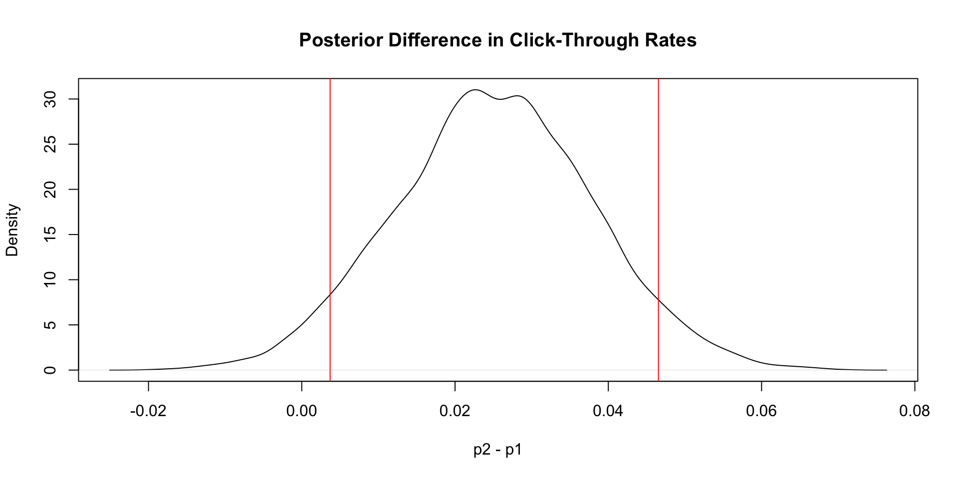
Lindley’s Paradox
Often evidence which, for a Bayesian statistician, strikingly supports the null leads to rejection by standard classical procedures.
- Do Bayes and Classical always agree?
Bayes computes the probability of the null being true given the data \(p ( H_0 | D )\). That’s not the p-value. Why?
Surely they agree asymptotically?
How do we model the prior and compute likelihood ratios \(L ( H_0 | D )\) in the Bayesianwork?
Bayes \(t\)-ratio
Edwards, Lindman and Savage (1963)
Simple approximation for the likelihood ratio. \[ L ( p_0 ) \approx \sqrt{2 \pi} \sqrt{n} \exp \left ( - \frac{1}{2} t^2 \right ) \]
- Key: Bayes test will have the factor \(\sqrt{n}\)
This will asymptotically favour the null.
- There is only a big problem when \(2 < t < 4\) – but this is typically the most interesting case!
Coin Tossing
Intuition: Imagine a coin tossing experiment and you want to determine whether the coin is “fair” \(H_0 : p = \frac{1}{2}\).
There are four experiments.
| Expt | 1 | 2 | 3 | 4 |
|---|---|---|---|---|
| n | 50 | 100 | 400 | 10,000 |
| r | 32 | 60 | 220 | 5098 |
| \(L(p_0)\) | 0.81 | 1.09 | 2.17 | 11.68 |
Coin Tossing
Implications:
Classical: In each case the \(t\)-ratio is approx 2. They we just \(H_0\) ( a fair coin) at the 5% level in each experiment.
Bayes: \(L ( p_0 )\) grows to infinity and so they is overwhelming evidence for \(H _ 0\). Connelly shows that the Monday effect disappears when you compute the Bayes version.