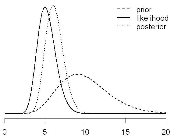
The posterior is proportional to the product of the likelihood and the priors.
Crucially: For certain choices of priors (like the Normal prior for \(\beta\) and Inverse Gamma for \(\sigma^2\)), the posterior has a known form (conjugate priors). This makes calculations easier. In other cases, we use approximation techniques.
Inference and Prediction
Inference: We’re interested in the posterior distribution \(P(\beta, \sigma^2 | Data)\). This tells us:
The most likely values of the coefficients (\(\beta\)).
The uncertainty associated with these estimates (captured by the spread of the posterior). The uncertainty in the noise variance (\(\sigma^2\)).
Prediction: Given a new input \(x^*\), we want to predict the corresponding output \(y^*\).
We use the posterior predictive distribution: \(P(y^* | x^*, Data)\)
This distribution integrates over the posterior distribution of the parameters:
This gives us a distribution over possible values of \(y^*\), not just a single point estimate. This captures the uncertainty in our prediction.
Advantages of Bayesian Linear Regression
Uncertainty Quantification: Provides a full probability distribution over the parameters and predictions, not just point estimates. This is crucial for decision-making.
Incorporation of Prior Knowledge: Allows us to incorporate prior beliefs about the parameters. This can be helpful when data is scarce or when we have expert knowledge.
Regularization: The prior acts as a natural regularizer, preventing overfitting (especially with informative priors). Similar in effect to ridge regression or lasso.
Model Comparison: Bayesian methods provide a framework for comparing different models (e.g., different sets of features) using the evidence (marginal likelihood).
Disadvantages and Challenges
Computational Complexity: Calculating the posterior (especially the evidence) can be computationally expensive, especially for complex models and large datasets. Approximation techniques like Markov Chain Monte Carlo (MCMC) are often required.
Prior Specification: Choosing appropriate priors can be challenging. Poorly chosen priors can lead to biased results. Sensitivity analysis (checking how the results change with different priors) is important.
Interpretation: While uncertainty quantification is a strength, interpreting posterior distributions can sometimes be less intuitive than interpreting point estimates.
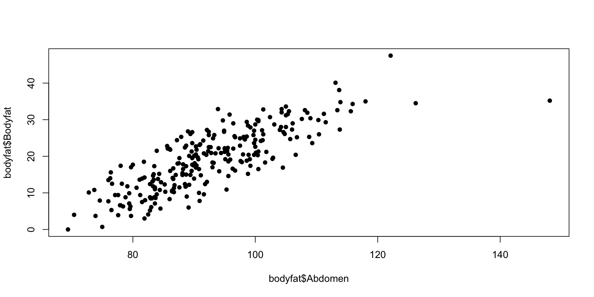
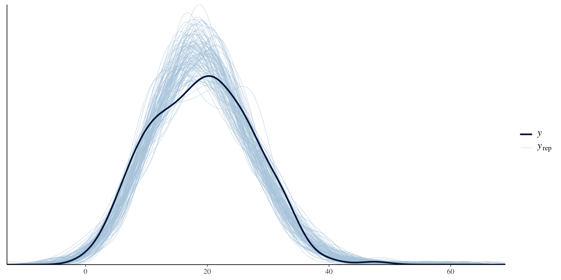
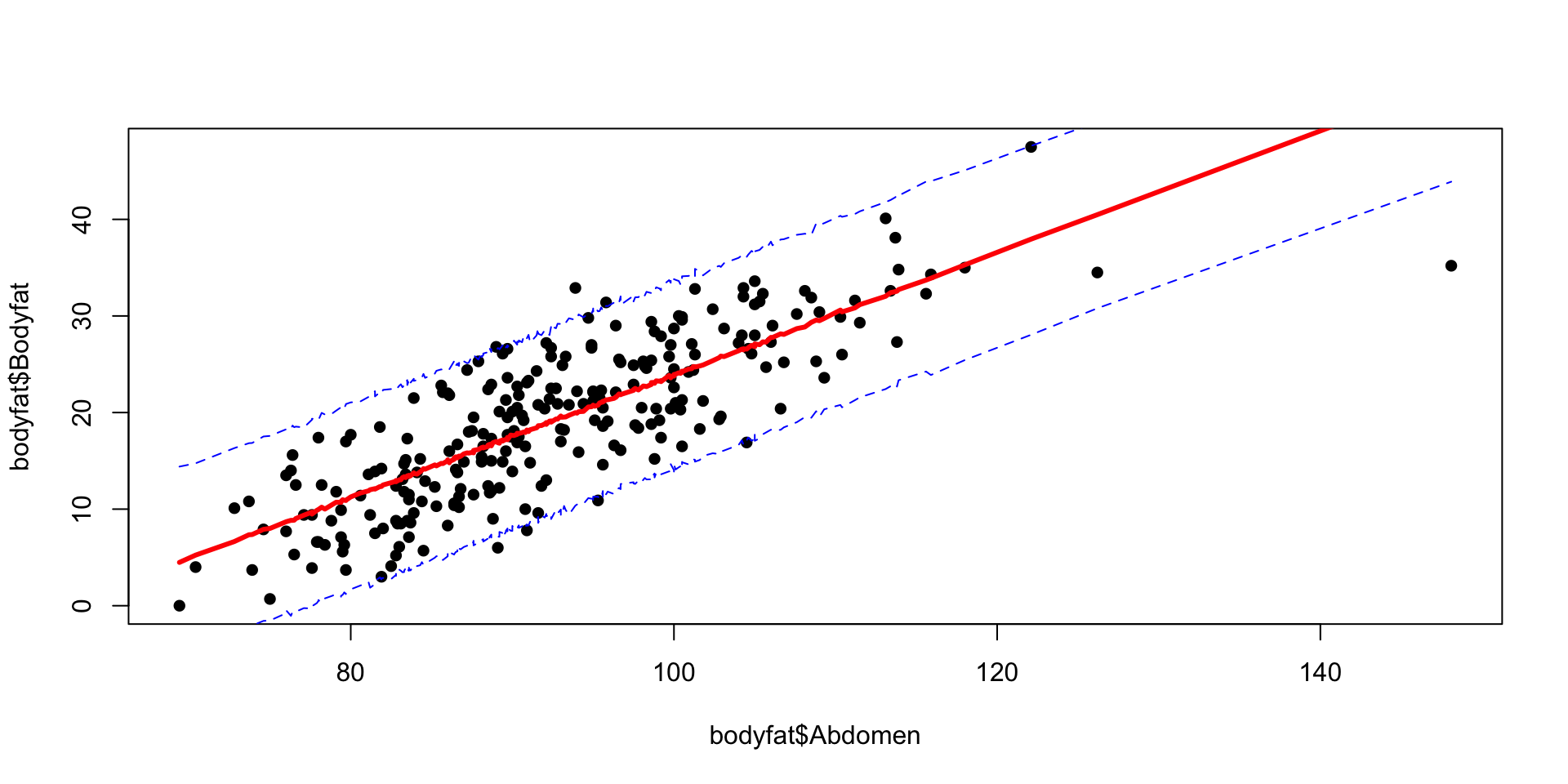
bodyfat example
Body fat is hard to measure
Can be predicted from abdominal circumference?
Use The data set bodyfat can be found from the library BAS.
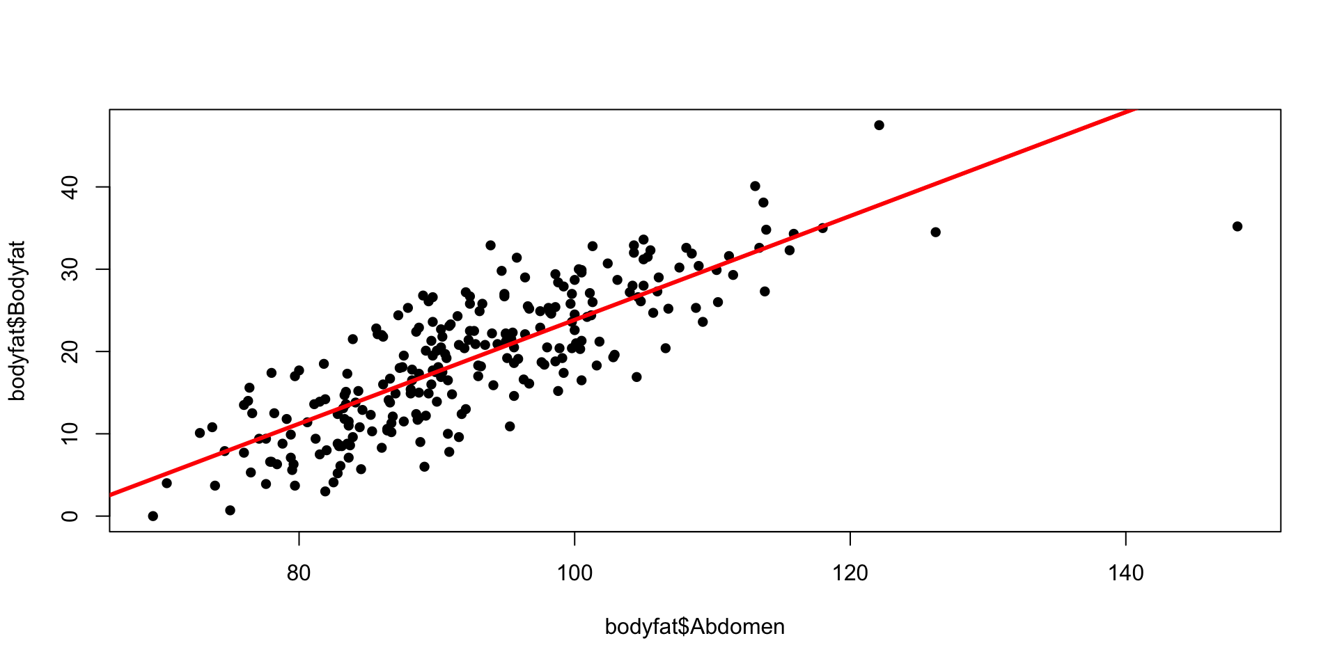
Bayesian Simple Linear Regression Using the Reference Prior
Likelihood: \[
Y_i~|~x_i, \alpha, \beta,\sigma^2~ \sim~ \textsf{Normal}(\alpha + \beta x_i, \sigma^2),\qquad i = 1,\cdots, n.
\] Priors: \[
p(\alpha,\beta \mid \sigma^2) \propto 1, \quad p(\sigma^2) \propto 1/\sigma^2.
\] Posterior: \[
\beta~|~y_1,\cdots,y_n ~\sim~ \textsf{t}\left(n-2,\ \hat{\beta},\ \frac{\hat{\sigma}^2}{\text{S}_{xx}}\right) = \textsf{t}\left(n-2,\ \hat{\beta},\ (\text{se}_{\beta})^2\right)
\]\(\hat{\beta}\) and \(\hat{\beta},\ (\text{se}_{\beta})^2\) are MLE estimates! For derivation, see Section 6.1.4 of An Introduction to Bayesian Thinking
The Bayesian posterior credible intervals for \(\alpha\) and \(\beta\) under the reference prior, are numerically equivalent to the confidence intervals from the classical frequentist OLS analysis!
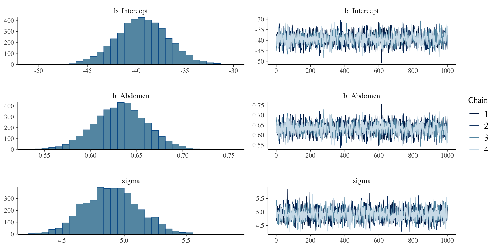
library(brms)priors <-c(prior(normal(0, 10), class ="b"), # Prior for coefficients (slope)prior(normal(0, 25), class ="Intercept"), # Prior for the interceptprior(student_t(3, 0, 100), class ="sigma") # Prior for the residual standard deviation)bodyfat.brms =brm(Bodyfat ~ Abdomen, data = bodyfat,family =gaussian(),prior = priors)
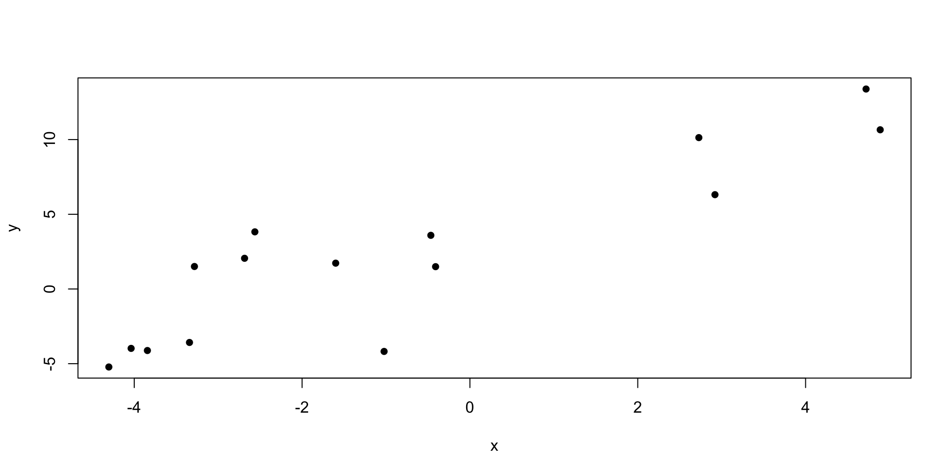
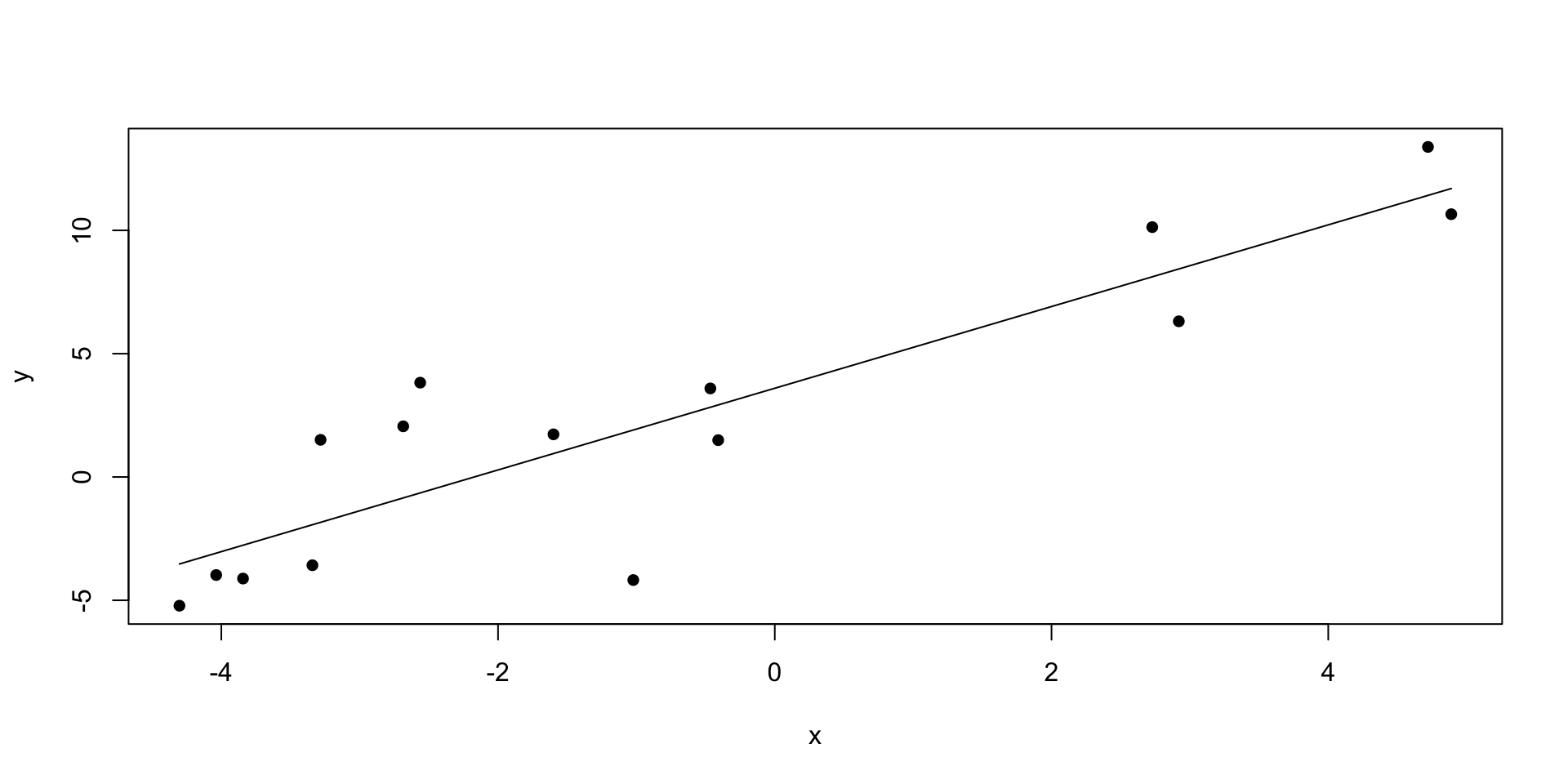
set.seed(7)true_intercept <-5true_slope <-2true_sigma <-3# Number of data points (intentionally small)n_data <-15# Generate predictor (x)x <-runif(n_data, min =-5, max =5)# Generate outcome (y) with noisey <- true_intercept + true_slope * x +rnorm(n_data, mean =0, sd = true_sigma)# Combine into a data framesim_data <-data.frame(x = x, y = y)plot(x, y, pch =16)
Classical Linear Regression
Code
ols_model <-lm(y ~ x, data = sim_data)summary(ols_model)
Call:
lm(formula = y ~ x, data = sim_data)

Residuals:
    Min      1Q  Median      3Q     Max
-6.0837 -1.5346 -0.8869  1.9904  4.4709

Coefficients:
            Estimate Std. Error t value Pr(>|t|)
(Intercept)   3.5984     0.7468   4.818 0.000336 ***
x             1.6563     0.2350   7.047 8.71e-06 ***
---
Signif. codes:  0 '***' 0.001 '**' 0.01 '*' 0.05 '.' 0.1 ' ' 1

Residual standard error: 2.795 on 13 degrees of freedom
Multiple R-squared:  0.7925,    Adjusted R-squared:  0.7766
F-statistic: 49.66 on 1 and 13 DF,  p-value: 8.712e-06
Code
x_vals <-seq(min(sim_data$x), max(sim_data$x), length.out =100)# Get OLS predictionsols_predictions <-predict(ols_model, newdata =data.frame(x = x_vals), interval ="confidence")ols_predictions <-as.data.frame(ols_predictions) # Convert to data frameols_predictions$x <- x_valsplot(x, y, pch =16)lines(x_vals,ols_predictions$fit)
Bayesian Linear Regression
Code
priors <-c(prior(normal(5, 1), class ="Intercept"), # Prior for interceptprior(normal(2, 1), class ="b"), # Prior for slopeprior(student_t(3, 0, 5), class ="sigma") # Prior for sigma (wider than the true value))# Fit the Bayesian model using brmsbayes_model <-brm(y ~ x,data = sim_data,family =gaussian(),prior = priors,seed =123)
 Family: gaussian
  Links: mu = identity; sigma = identity
Formula: y ~ x
   Data: sim_data (Number of observations: 15)
  Draws: 4 chains, each with iter = 2000; warmup = 1000; thin = 1;
         total post-warmup draws = 4000

Regression Coefficients:
          Estimate Est.Error l-95% CI u-95% CI Rhat Bulk_ESS Tail_ESS
Intercept     4.71      0.73     3.36     6.20 1.00     2856     2479
x             1.68      0.26     1.16     2.21 1.00     2984     2130

Further Distributional Parameters:
      Estimate Est.Error l-95% CI u-95% CI Rhat Bulk_ESS Tail_ESS
sigma     3.22      0.72     2.17     5.00 1.00     2474     2322

Draws were sampled using sampling(NUTS). For each parameter, Bulk_ESS
and Tail_ESS are effective sample size measures, and Rhat is the potential
scale reduction factor on split chains (at convergence, Rhat = 1).
          Estimate Est.Error l-95% CI u-95% CI     Rhat Bulk_ESS Tail_ESS
Intercept 4.712777 0.7325443 3.358504 6.198919 1.001263 2855.809 2478.723
x         1.680288 0.2634961 1.161723 2.207987 1.001100 2984.003 2129.753
Code
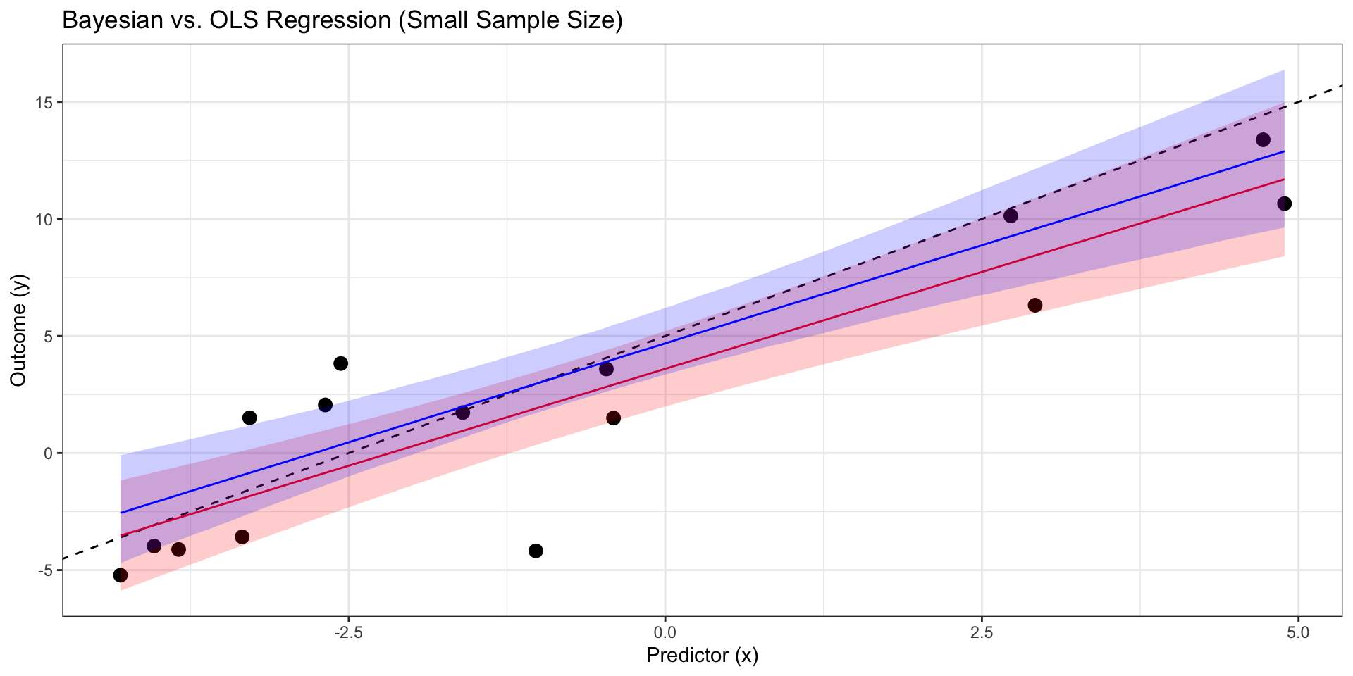
# Get Bayesian predictions (posterior draws of the expected value, epred)bayes_predictions <-posterior_epred(bayes_model, newdata =data.frame(x = x_vals))quntiles =apply(bayes_predictions, 2, function(x) quantile(x, c(0.025, 0.5,0.975)))bayes_pred_summary=as.data.frame(t(quntiles)) #col.names=c("lwr","med","upr")colnames(bayes_pred_summary) =c("lower","med","upper")bayes_pred_summary$x <- x_vals# Plot the data, OLS fit, and Bayesian fitggplot(sim_data) +geom_point(aes(x = x, y = y),size =3) +# True regression line (for comparison)geom_abline(intercept = true_intercept, slope = true_slope, color ="black", linetype ="dashed") +# OLS regression line and confidence intervalgeom_line(data = ols_predictions, aes(x = x, y = fit), color ="red") +geom_ribbon(data = ols_predictions, aes(x=x, ymin = lwr, ymax = upr), fill ="red", alpha =0.2) +# Bayesian regression line and credible intervalgeom_line(data = bayes_pred_summary, aes(x = x, y = med), color ="blue") +geom_ribbon(data = bayes_pred_summary, aes(x=x, ymin = lower, ymax = upper), fill ="blue", alpha =0.2) +labs(title ="Bayesian vs. OLS Regression (Small Sample Size)",x ="Predictor (x)",y ="Outcome (y)") +theme_bw()
Sparsity Inducing Prior
Code
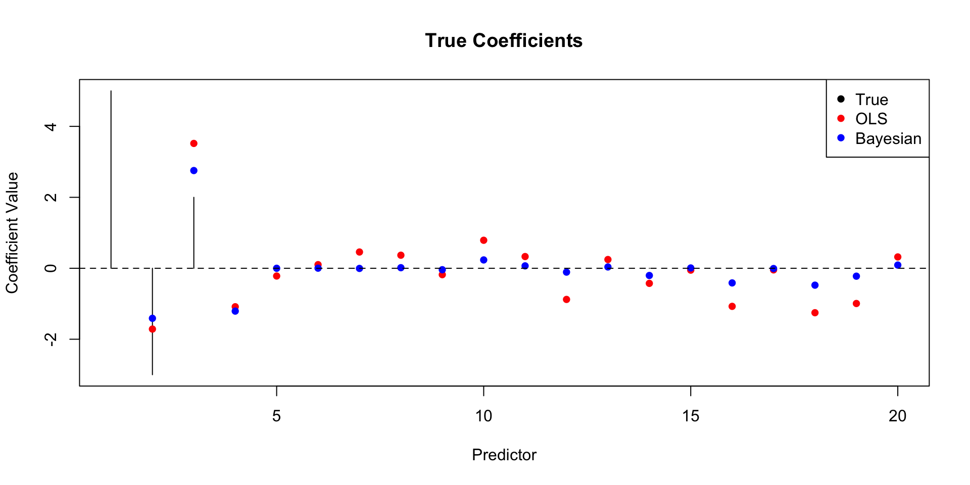
# Simulate data with some true coefficients and some noiseset.seed(7) # For reproducibilityn <-100# Number of observationsp <-20# Number of predictors (some relevant, some not)true_beta <-c(5, -3, 2, 0, 0, 0, 0, 0, 0, 0, 0, 0, 0, 0, 0, 0, 0, 0, 0, 0) # Only first 3 are truly non-zeroX <-matrix(rnorm(n * p), n, p)y <- X %*% true_beta +rnorm(n, 0, 5) # Adding noise# Fit a standard linear regression (OLS)ols_model <-lm(y ~ X-1)# Fit a Bayesian linear regression with shrinkage (using the 'BAS' package)# Install if you don't have it: install.packages("BAS")library(BAS)# Define prior (we'll use a g-prior which is common for shrinkage)# 'gprior' is common for shrinkage# 'bic' is another option that often works well# 'hyper-g' is another good choicebas_model <-bas.lm(y ~ X-1, prior ="g-prior", modelprior =uniform())# Examine coefficientsols_coef <-coef(ols_model)bas_coef <-coefficients(bas_model) # These are *posterior means*# Plot the coefficients to visualize shrinkageplot(1:p, true_beta, type ="h", ylab ="Coefficient Value", xlab ="Predictor", main ="True Coefficients")points(1:p, ols_coef, col ="red", pch =16) # OLSpoints(1:p, bas_coef$postmean, col ="blue", pch =16) # Bayesianabline(h =0, lty =2)legend("topright", legend =c("True", "OLS", "Bayesian"), col =c("black", "red", "blue"), pch =16)
What are Random Intercepts Models?
Extension of Linear Regression: Deals with clustered or hierarchical data.
Clustered Data: Observations are grouped within clusters (e.g., students within schools, patients within hospitals, measurements over time within individuals).
Problem with Standard Regression: Ignores the clustering, leading to:
Underestimated standard errors (and thus, inflated Type I error rates - false positives).
Incorrect conclusions about the significance of predictors.
Random Intercepts: Assume each cluster has its own intercept, which is drawn from a distribution (usually normal). This accounts for between-cluster variability.
\(\gamma\) (Fixed Intercept): The average outcome when the predictor \(x\) is zero (and across all clusters).
\(\beta_1\) (Fixed Slope): The change in the outcome for a one-unit increase in \(x\), within any given cluster.
\(\sigma^2_u\) (Random Intercept Variance): The variance of the cluster-specific intercepts. Indicates the amount of between-cluster variability. A larger \(\sigma^2_u\) means more variation between clusters.
\(\sigma^2_e\) (Residual Variance): The variance of the individual-level errors. Indicates within-cluster variability.
Intraclass Correlation Coefficient (ICC):
\(ICC = \sigma^2_u / (\sigma^2_u + \sigma^2_e)\)
Represents the proportion of total variance that is due to between-cluster differences. Ranges from 0 to 1. Higher ICC means more clustering.
Example: Student Test Scores in Schools
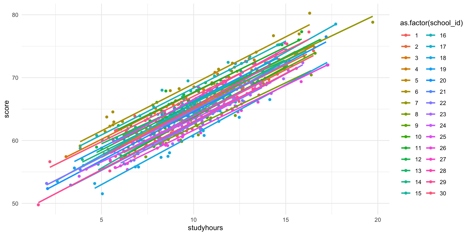
Data: We have data on student test scores (\(score\)) and a student-level predictor (e.g., hours of study, \(studyhours\)). Students are nested within schools.
Research Question: Does the number of study hours predict test scores, accounting for the fact that students are clustered within schools?
# Install and load necessary packageslibrary(lme4)library(lmerTest)library(ggplot2)# Create some simulated data (for reproducibility)set.seed(123)n_schools <-30# Number of schoolsn_students_per_school <-20# Students per schooln_total <- n_schools * n_students_per_schoolschool_effects <-rnorm(n_schools, mean =0, sd =2) # School random effectsstudent_data <-data.frame(school_id =rep(1:n_schools, each = n_students_per_school),studyhours =rnorm(n_total, mean =10, sd =3),error =rnorm(n_total, mean=0, sd =1))# Generate scores based on the modelstudent_data$score <-50+1.5* student_data$studyhours + school_effects[student_data$school_id] + student_data$errorhead(student_data)
# Plot the data and use school_id for color and add a linear model to fit the data for each schoolggplot(student_data, aes(x = studyhours, y = score, color =as.factor(school_id))) +geom_point() +geom_smooth(method ="lm", se =FALSE) +theme_minimal()
R Demonstration - Fit the Model
Code
# Fit the random intercepts model using lmer()model <-lmer(score ~ studyhours + (1| school_id), data = student_data)# View the model summarysummary(model)
Linear mixed model fit by REML. t-tests use Satterthwaite's method [
lmerModLmerTest]
Formula: score ~ studyhours + (1 | school_id)
   Data: student_data

REML criterion at convergence: 1846.4

Scaled residuals:
     Min       1Q   Median       3Q      Max
-2.71647 -0.68621  0.01679  0.64918  2.99847

Random effects:
 Groups    Name        Variance Std.Dev.
 school_id (Intercept) 3.845    1.961
 Residual              1.014    1.007
Number of obs: 600, groups:  school_id, 30

Fixed effects:
             Estimate Std. Error        df t value Pr(>|t|)
(Intercept)  49.84593    0.38800  38.91559   128.5   <2e-16 ***
studyhours    1.50785    0.01432 569.50545   105.3   <2e-16 ***
---
Signif. codes:  0 '***' 0.001 '**' 0.01 '*' 0.05 '.' 0.1 ' ' 1

Correlation of Fixed Effects:
           (Intr)
studyhours -0.371
R Demonstration - Interpreting the Output
Fixed Effects:
Intercept \((\gamma)\): Estimated average score when \(studyhours\) is 0.
studyhours \((\beta_1)\): Estimated increase in score for each additional hour of study. The p-value indicates if this effect is statistically significant.
Random Effects:
Variance (school_id) \(\sigma^2_u\): Estimated variance of the school-specific intercepts.
Variance (Residual) \(\sigma^2_e\): Estimated variance of the individual-level errors.
ICC Calculation*
VarCorr(model)
 Groups    Name        Std.Dev.
 school_id (Intercept) 1.9609
 Residual              1.0072
sigma2u <-2.384#From the output of VarCorr(model), school_id variancesigma2e <-0.962#From the output of VarCorr(model), residual varianceicc <- sigma2u / (sigma2u + sigma2e)print(paste("ICC:", round(icc, 3)))
[1] "ICC: 0.712"
R Demonstration - Visualizing the Model
Code
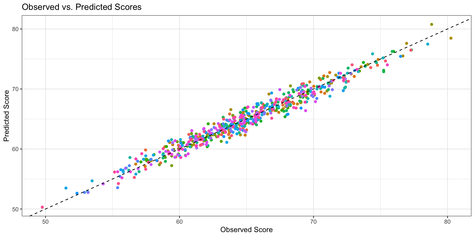
# Get predicted values for each studentstudent_data$predicted <-predict(model)# Plot observed vs. predicted values, colored by schoolggplot(student_data, aes(x = score, y = predicted, color =factor(school_id))) +geom_point() +geom_abline(intercept =0, slope =1, linetype ="dashed") +# Add a diagonal linelabs(title ="Observed vs. Predicted Scores",x ="Observed Score",y ="Predicted Score",color ="School ID") +theme_bw() +theme(legend.position ="none") #remove legend because too many schools
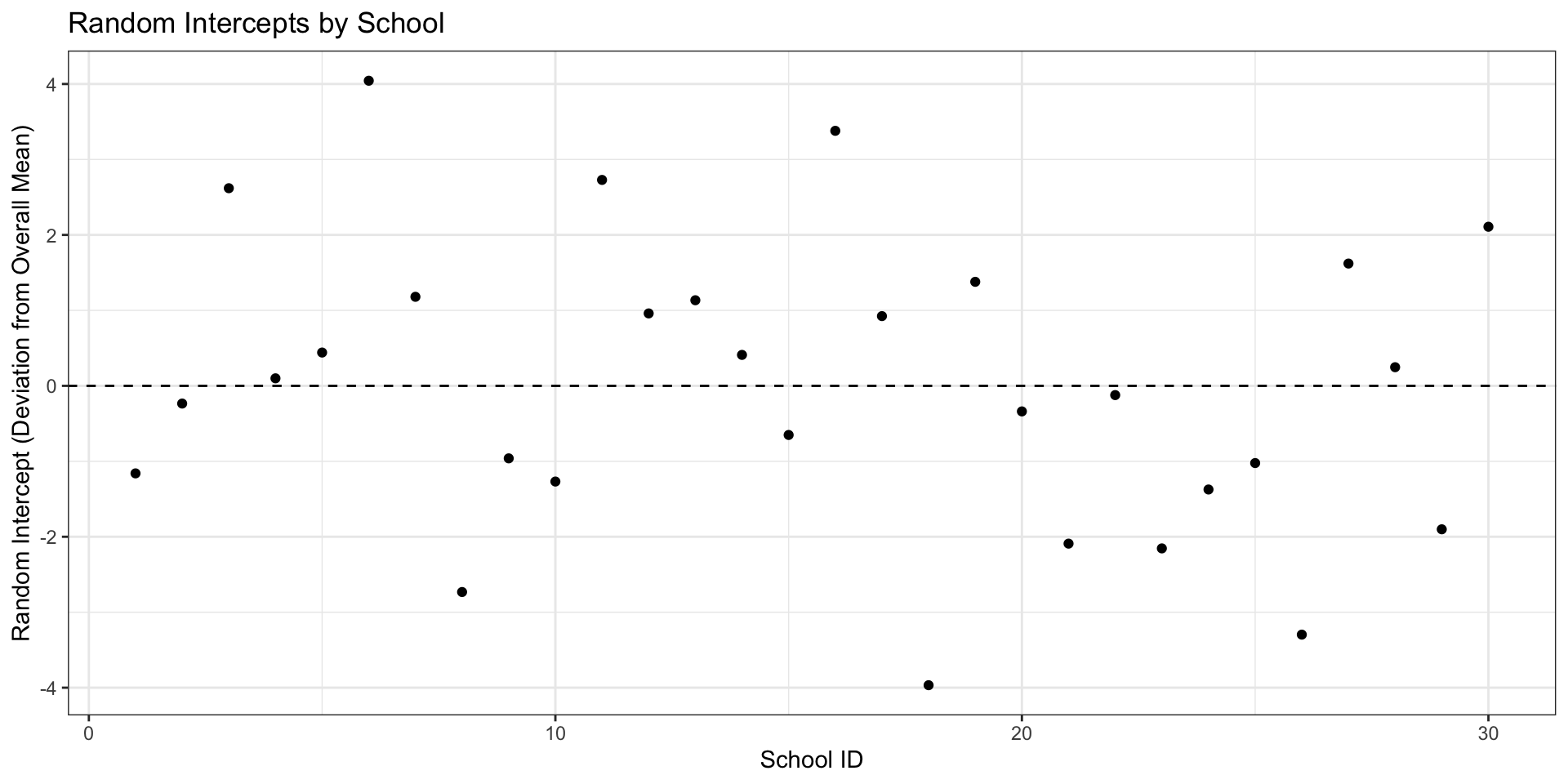
Plot random intercepts for each school
Code
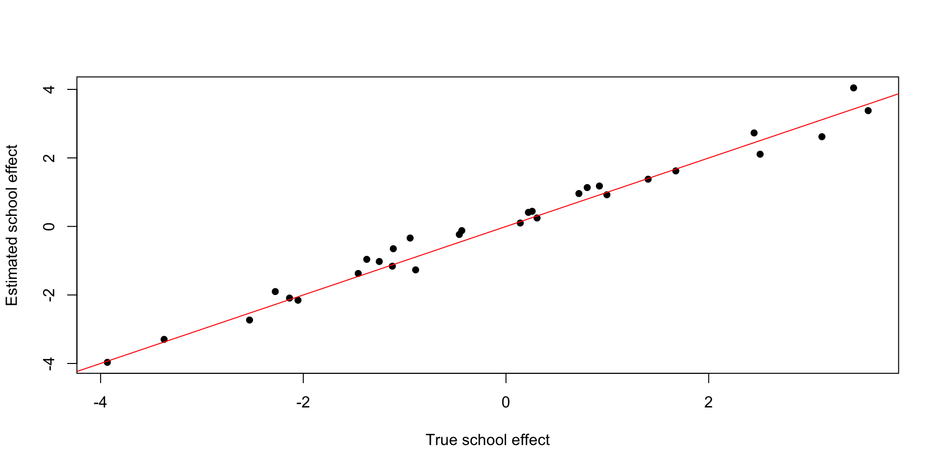
plot(school_effects,ranef(model)$school_id[,1], pch=16, xlab="True school effect", ylab="Estimated school effect")abline(a=0,b=1,col="red")
Plot random intercepts for each school
Code
ranef_df <-as.data.frame(ranef(model)$school_id)ranef_df$school_id <-1:nrow(ranef_df)ggplot(ranef_df, aes(x = school_id, y =`(Intercept)`)) +geom_point() +geom_hline(yintercept =0, linetype ="dashed") +labs(title ="Random Intercepts by School",x ="School ID",y ="Random Intercept (Deviation from Overall Mean)") +theme_bw()
Comparing to a Simple Linear Model
Code
# Fit a simple linear regression (ignoring clustering)simple_model <-lm(score ~ studyhours, data = student_data)# summary(simple_model) # Compare standard errorscoef(summary(model)) # Random intercepts model
             Estimate Std. Error        df  t value     Pr(>|t|)
(Intercept) 49.845931 0.38799971  38.91559 128.4690 9.116905e-53
studyhours   1.507846 0.01431791 569.50545 105.3119 0.000000e+00
Code
coef(summary(simple_model)) # Simple linear model
            Estimate Std. Error  t value      Pr(>|t|)
(Intercept) 50.10072 0.31835002 157.3762  0.000000e+00
studyhours   1.48248 0.03043469  48.7102 2.579971e-210
Notice how the standard error for \(studyhours\) is smaller in the simple linear model. This is because it doesn’t account for the clustering, leading to an overestimation of the precision of the estimate.
Model Extensions and Considerations
Random Slopes: Allow the effect of \(studyhours\) to vary across schools (not just the intercept). This is done by adding \((studyhours | school_id)\) to the \(lmer\) formula.
Crossed Random Effects: When observations have multiple sources of clustering (e.g., students nested within schools AND neighborhoods).
More Complex Models: Can include multiple predictors at both the individual and cluster levels.
Model Selection: Use AIC, BIC, or likelihood ratio tests to compare different models (e.g., with and without random intercepts, with and without random slopes).
Assumptions: Linearity, normality of residuals and random effects, independence of errors (within clusters, after accounting for the random effects), homoscedasticity. Check these assumptions using diagnostic plots.
Software:\(lme4\) is the most common R package. Other options include \(nlme\), \(brms\) (for Bayesian mixed models), and \(glmmTMB\).
Sweet Spot For Bayesian Regression
When you have a good prior knowledge about the parameters (e.g. from previous studies, expert opinion, etc.)
When you want to quantify uncertainty in your estimates
When you know that many of the predictors are not important (sparsity)
When dealing with small sample sizes
Hierarchical data (e.g. students within schools, patients within hospitals)
Modeling nested relationships
Sharing Information Across Groups
When you want to compare multiple models
Examples where Bayesian Regression is Useful
Medical Trials: Incorporating prior knowledge about treatment effects.
Marketing: Predicting customer behavior with sparse data.
Educational studies: Analyzing student performance within classrooms and schools, while accounting for variations in teacher effectiveness and school resources.
Social sciences: Examining individual behavior within different communities or regions, while accounting for contextual factors and cultural differences.
Ecology: Modeling species populations within different habitats or ecosystems, while considering environmental variations and species interactions
Bayesian Additive Regression Trees (BART)
Core Ideas of BART
BART is a non-parametric Bayesian model used for both regression and classification.
Its core idea is to represent a complex relationship between predictors (\(X\)) and a response variable (\(Y\)) as a sum of many simple regression trees.
Each tree is a “weak learner.” It’s typically a small decision tree, often with only a - - Ensemble Power: The sum of the predictions from many of these weak learners creates a powerful and flexible model. This is similar in spirit to boosted trees (like XGBoost or LightGBM), but BART’s Bayesian nature provides important advantages.
\(f(X_i)\) is the overall prediction function, which is the sum of the tree predictions.
\(\epsilon_i\) is the error term, assumed to be normally distributed with mean 0 and variance \(\sigma^2\).
\(m\) is the number of trees in the ensemble (a crucial hyperparameter).
\(g(X_i; T_j, M_j)\) is the prediction from the j-th tree.
\(T_j\) represents the tree structure (the splitting rules). It defines the splits based on the predictor variables and their values.
\(M_j = {\mu_{1j}, \mu_{2j}, ..., \mu_{b_j j}}\) represents the set of terminal node parameters (the “leaf values”) for the j-th tree. \(b_j\) is the number of terminal nodes (leaves) in tree \(T_j\). Each leaf gets assigned a constant value (), which is the prediction for any observation that falls into that leaf.
Diagram
Code
graph TB subgraph Input X[Predictors] end subgraph BARTModel Tree1((Tree 1)) --> Sum Tree2((Tree 2)) --> Sum TreeM((Tree M)) --> Sum Sum[Sum of Trees] end subgraph Output fX["f(X) - Prediction"] endInput --> BARTModelBARTModel --> OutputfX --> Y["Y= f(X) + ε"]
graph TB
    subgraph Input
        X[Predictors]
    end
    subgraph BARTModel
        Tree1((Tree 1)) --> Sum
        Tree2((Tree 2)) --> Sum
        TreeM((Tree M)) --> Sum
        Sum[Sum of Trees]
    end
    subgraph Output
        fX["f(X) - Prediction"]
    end
Input --> BARTModel
BARTModel --> Output
fX --> Y["Y= f(X) + ε"]
Single Node
Example of a single tree (\(T_j\)):
Code
graph TD
    A[X1 < 3] --> B{Yes};
    A --> C{No};
    B --> D[X2 > 7];
    C --> E[X2 > 7];
    D --> F("$$\mu_1$$");
    D --> G("$$\mu2$$");
    E --> H("$$\mu3$$");
    E --> I("$$\mu4$$");
graph TD
    A[X1 < 3] --> B{Yes};
    A --> C{No};
    B --> D[X2 > 7];
    C --> E[X2 > 7];
    D --> F("$$\mu_1$$");
    D --> G("$$\mu2$$");
    E --> H("$$\mu3$$");
    E --> I("$$\mu4$$");
Bayesian Priors (The Bayesian Part)
Prior on Tree Structure (\(T_j\)): prefer smaller trees: regularization and prevents overfitting. The prior for node splitting and choosing a particular predictor variable for splitting.
Prior on Leaf Parameters (\(M_j\)): A common choice is a normal prior: \[
\mu_{kj} ~ N(0, \sigma_\mu^2)
\] Prior 0: the trees are encouraged to make small “corrections” rather than large jumps.
Prior on Error Variance (^2): An inverse-gamma prior is often used: \[
\sigma^2 ~ InverseGamma(\nu/2, \nu\lambda/2)
\]
\(\nu\) (degrees of freedom) and \(\lambda\) (scale) are hyperparameters. This prior allows the model to learn the appropriate level of noise in the data.
Inference (MCMC)
Because of the complex structure and the priors, we can’t directly calculate the posterior distribution of the parameters \((T_j, M_j, \sigma^2)\).
Instead, BART uses Markov Chain Monte Carlo (MCMC) methods, specifically a Metropolis-within-Gibbs sampler, to draw samples from the posterior distribution.
The MCMC algorithm iteratively updates: \(T_j\) and \(M_j\)
Iterative Updates
Each Tree (T_j and M_j): For each tree, the algorithm proposes changes to the tree structure (growing, pruning, changing splitting rules) and the leaf values. These proposals are accepted or rejected based on how well they improve the fit to the data, given the current state of all the other trees. This is the “backfitting” part of BART – each tree is adjusted to account for the predictions of the other trees.
The Error Variance (^2): The error variance is updated based on the residuals (the difference between the observed \(Y\) values and the current model predictions).
The result of the MCMC process is a collection of samples from the posterior distribution of the model parameters.
Example in R (BART package)
Code
# Install the BART package if you haven't already# install.packages("BART")library(BART)library(MASS) #For Boston Housing# Load the Boston Housing datasetdata(Boston)X <- Boston[, -14] # Predictors (all columns except 'medv')Y <- Boston[, 14] # Response variable ('medv' - median house value)# Fit the BART model# - ntree: Number of trees (m in the formulas)# - ndpost: Number of posterior samples to keep (after burn-in)# - nskip: Number of burn-in iterations to discardbart_model <-gbart(x.train = X, y.train = Y, ntree =50, ndpost =1000, nskip =500)
*****Calling gbart: type=1
*****Data:
data:n,p,np: 506, 13, 0
y1,yn: 1.467194, -10.632806
x1,x[n*p]: 0.006320, 7.880000
*****Number of Trees: 50
*****Number of Cut Points: 100 ... 100
*****burn,nd,thin: 500,1000,1
*****Prior:beta,alpha,tau,nu,lambda,offset: 2,0.95,1.59099,3,4.38629,22.5328
*****sigma: 4.745298
*****w (weights): 1.000000 ... 1.000000
*****Dirichlet:sparse,theta,omega,a,b,rho,augment: 0,0,1,0.5,1,13,0
*****printevery: 100

MCMC
done 0 (out of 1500)
done 100 (out of 1500)
done 200 (out of 1500)
done 300 (out of 1500)
done 400 (out of 1500)
done 500 (out of 1500)
done 600 (out of 1500)
done 700 (out of 1500)
done 800 (out of 1500)
done 900 (out of 1500)
done 1000 (out of 1500)
done 1100 (out of 1500)
done 1200 (out of 1500)
done 1300 (out of 1500)
done 1400 (out of 1500)
time: 2s
trcnt,tecnt: 1000,0
Code
# Make predictions on the training data (or you could use a separate test set)predictions <-predict(bart_model, newdata = X) # This returns a matrix: rows=observations, cols=posterior samples
*****In main of C++ for bart prediction
tc (threadcount): 1
number of bart draws: 1000
number of trees in bart sum: 50
number of x columns: 13
from x,np,p: 13, 506
***using serial code
Code
# Calculate the mean prediction for each observationmean_predictions <-colMeans(predictions)# Calculate 95% credible intervalscredible_intervals <-apply(predictions, 2, quantile, probs =c(0.025, 0.975))
Example in R (BART package)
Code
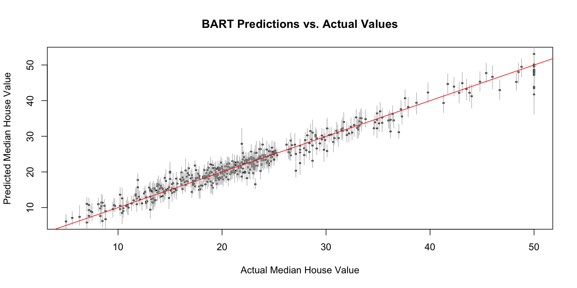
# Plot predictions vs. actual values (with credible intervals)plot(Y, mean_predictions, main ="BART Predictions vs. Actual Values",xlab ="Actual Median House Value", ylab ="Predicted Median House Value",pch=16, cex=0.5)segments(Y, credible_intervals[1, ], Y, credible_intervals[2, ], col ="gray")abline(0, 1, col ="red") # Add a y=x line for reference
Example in R (BART package)
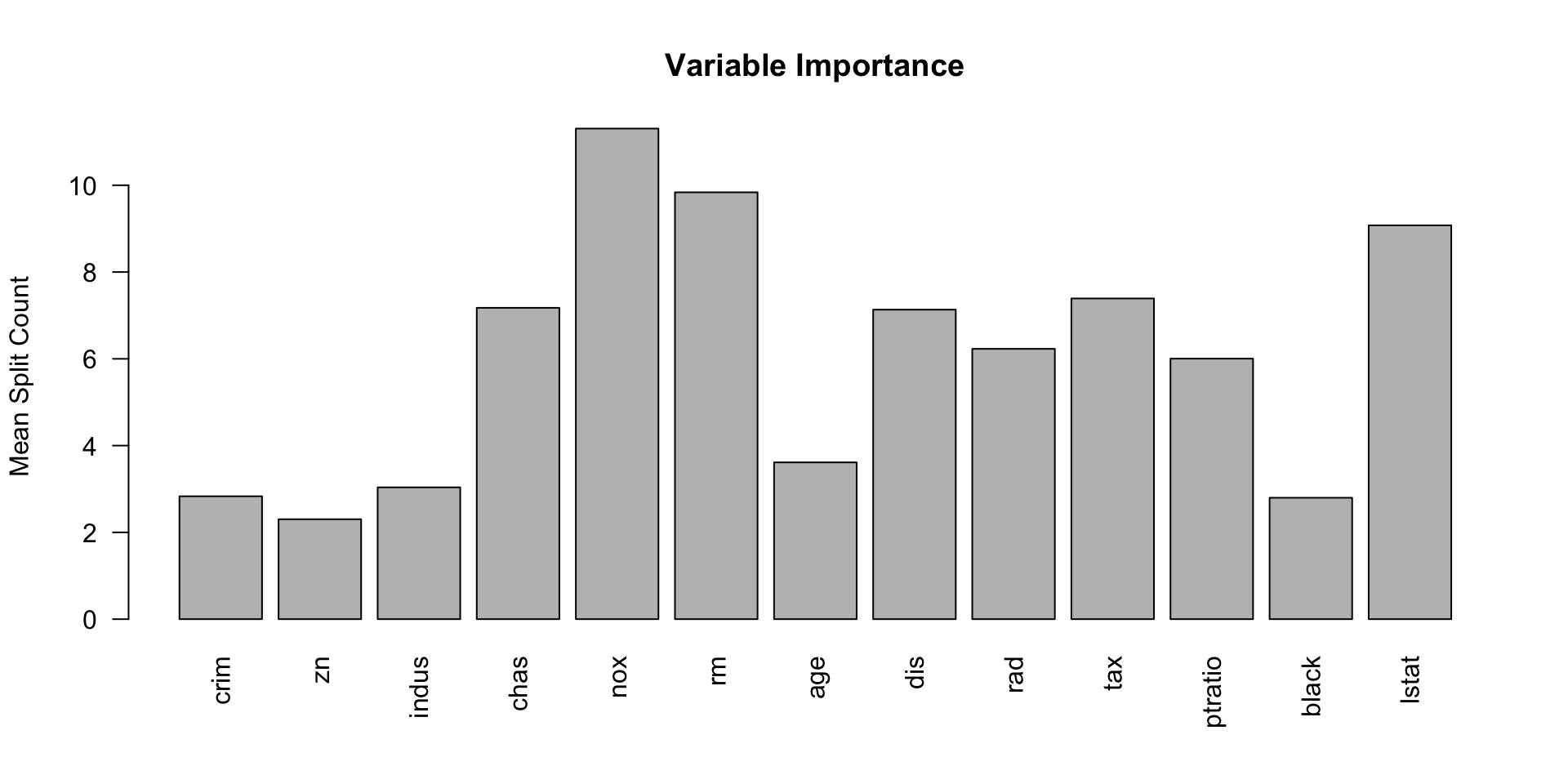
Code
# Variable Importancevar_importance <- bart_model$varcount # Number of times each variable was used for splittingvar_importance_mean <-colMeans(var_importance)barplot(var_importance_mean, names.arg =colnames(X), las =2,main ="Variable Importance", ylab ="Mean Split Count")
Example in R (BART package)
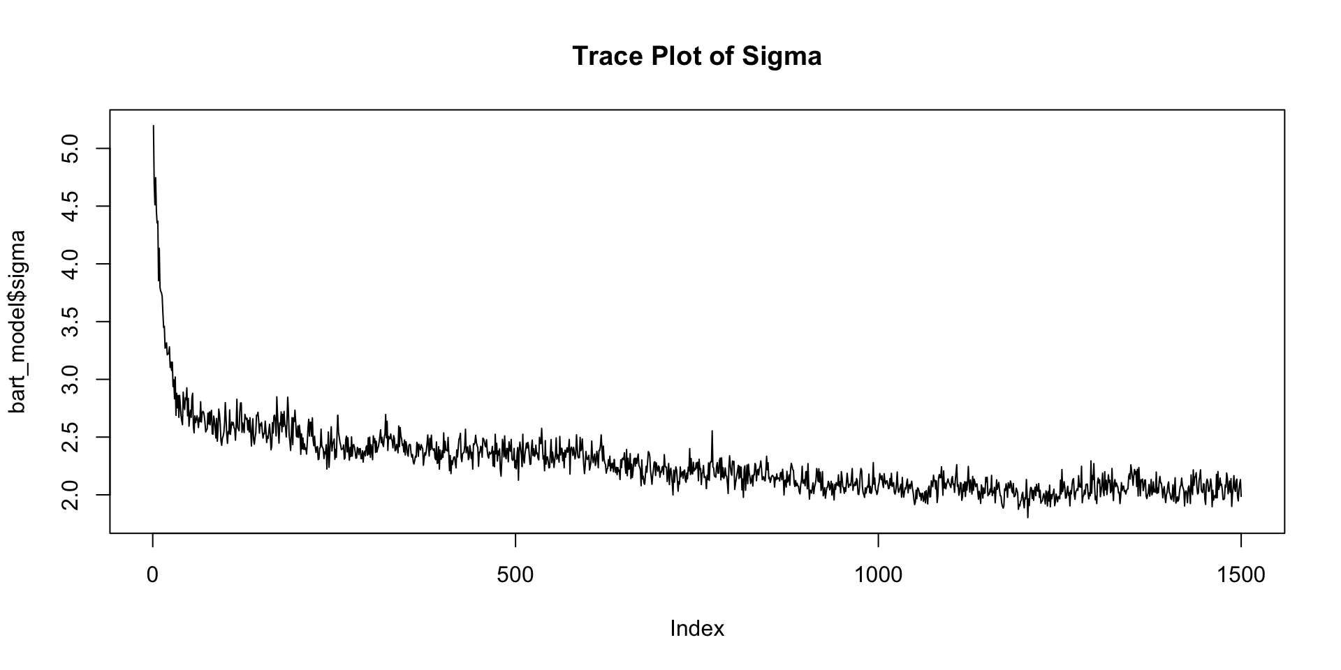
Code
# Check convergence (trace plots - should look like "fuzzy caterpillars")plot(bart_model$sigma, type ="l", main ="Trace Plot of Sigma") #sigma plot
Example in R (BART package)
Code
# Example for prediction with new datanew_data <- X[1:5,] # Lets pretend these are five new datapointsnew_predictions <-predict(bart_model, newdata = new_data)
*****In main of C++ for bart prediction
tc (threadcount): 1
number of bart draws: 1000
number of trees in bart sum: 50
number of x columns: 13
from x,np,p: 13, 5
***using serial code
Code
new_mean_predictions <-colMeans(new_predictions)new_credible_intervals <-apply(new_predictions, 2, quantile, probs =c(0.025, 0.975))print(new_mean_predictions) #print mean prediction for new data
[1] 23.27826 21.08262 33.92599 33.88669 34.63011
Code
print(new_credible_intervals) # print the CI for new data
Flexibility: Can capture complex non-linear relationships and interactions between predictors.
Regularization: The Bayesian priors and the sum-of-trees structure provide built-in regularization, reducing the risk of overfitting.
Uncertainty Quantification: Provides credible intervals, giving a measure of uncertainty in the predictions.
Variable Importance: Provides a natural way to assess the importance of different predictors.
Good Default Performance: Often performs well with minimal tuning of hyperparameters (although tuning can further improve performance).
Disadvantages and Considerations**
Computational Cost: MCMC sampling can be computationally expensive, especially for large datasets and a large number of trees.
Interpretability: While variable importance is helpful, the complex ensemble of trees can be difficult to interpret directly (compared to, say, a linear regression model). Partial dependence plots can help.
Hyperparameter Tuning: While BART often works well with defaults, tuning \(ntree\), \(ndpost\), \(nskip\), and the prior parameters can further improve performance. Cross-validation is recommended for this. The \(BART\) package provides functions for this.
Missing data: Handling missing data in BART could require imputation strategies before modelling.
MCMC Training Process
Code
graph LR
    subgraph TrainingData
        X_train[Training Predictors]
        Y_train[Training Response]
    end
    subgraph BARTModel
        Trees["Multiple Trees (Tj, Mj)"]
    end
     subgraph MCMC
        MCMCIterations[MCMC Samples of Trees]
    end
    subgraph NewData
        X_new[New Predictors]
    end
    subgraph Prediction
        Predictions[Multiple Predictions]
        MeanPrediction[Mean Prediction]
        CredibleIntervals[Credible Intervals]
    end

    TrainingData --> BARTModel
    BARTModel --> MCMCIterations
    X_new --> MCMCIterations
    MCMCIterations --> Predictions
    Predictions --> MeanPrediction
    Predictions --> CredibleIntervals
Bill Gates: 12/11/2009: “I’m most worried about a worldwide Pandemic”
Early-period Pandemics
Dates
Size of Mortality
Plague of Athens
430 BC
25% population.
Black Death
1347
30% Europe
London Plague
1666 2
0% population
Recent Flu Epidemics
Dates 1900-2010
Size
Spanish Flu
1918-19 40-
50 million
Asian Flu
H2N2, 1957-58 2
million
Hong Kong Flu
H3N2, 1968-69 6
million
Spanish Flu killed more than WW1
H1N1 Flu 2009: \(18,449\) people killed World wide:
SEIR Epidemic Models
Growth “self-reinforcing”: More likely if more infectants
An individual comes into contact with disease at rate \(\beta_1\)
The susceptible individual contracts the disease with probability \(\beta_2\)
Each infectant becomes infectious with rate \(\alpha\) per unit time
Each infectant recovers with rate \(\gamma\) per unit time
\(S_t + E_t + I_t + R_t = N\)
Current Models: SEIR
susceptible-exposed-infectious-recovered model
Dynamic models that extend earlier models to include exposure and recovery.
The coupled SEIR model: \(\dot{S} = -\beta S I\) \(\dot{E} = \beta S I - \alpha E\) \(\dot{I} = \alpha E -\gamma I\) \(\dot{R} = \gamma I\)
Infectious disease models
Daniel Bernoulli’s (1766) first model of disease transmission in smallpox:
“I wish simply that, in matters which so closely concern the well being of the human race, no decision shall be made without all knowledge which a little analysis and calculation can provide”
R.A. Ross, (Nobel Medicine winner, 1902) – math model of malaria transmission, which ultimately lead to malaria control.
Ross-McDonald model
Kermack and McKendrick: susceptible-infectious-recovered (SIR)
London Plague 1665-1666; Cholera: London 1865, Bombay, 1906.
Example: London Plague, 1666: Village Eyam nr. Sheffield
Model of transmission from Infectants, \(I\), to susceptibles, \(S\).
Date 1666 Su
sceptibles In
fectives
Initial
254
7
July 3
235 15
July 19
201 22
Aug 3 1
53 29
Aug 19
121 21
Sept 3
108 8
Sept 19
97 8
Oct 3
–
–
Oct 19
83 0
Initial Population \(N=261=S_0\); Final population \(S_\infty = 83\).
Modeling Growth: SI
Coupled Differential eqn \(\dot{S} = - \beta SI , \dot{I} = ( \beta S - \alpha ) I\)
\[
\theta \sim N(m_0, C_0)
\]\[
x_t = \theta + w_t,~~~w_t \sim N(0,\sigma^2)
\]\[
x_1,x_2,\ldots \mid \theta \sim N(\theta,\sigma^2)
\] The prior variance \(C_0\) might be quite large if you are very uncertain about your guess \(m_0\)
Given the measurements \(x^n = (x_1,\ldots,x_n)\), you update your opinion about \(\theta\) computing its posterior density, using the Bayes formula
We will look at the Gaussian distribution from a Bayesian point of view. In the standard form, the likelihood has two parameters, the mean \(\mu\) and the variance \(\sigma^2\)\[
p(x^n | \mu, \sigma^2) \propto \dfrac{1}{\sigma^n}\exp\left(-\dfrac{1}{2\sigma^2}\sum_{i=1}^n(x_i-\mu)^2\right)
\]
Normal Prior
In case when we know the variance \(\sigma^2\), but do not know mean \(\mu\), we assume \(\mu\) is random. To have conjugate prior we choose \[
p(\mu | \mu_0, \sigma_0) \propto \dfrac{1}{\sigma_0}\exp\left(-\dfrac{1}{2\sigma_0^2}(\mu-\mu_0^2)\right)
\] In practice, when little is known about \(\mu\), it is common to set the location hyper-parameter to zero and the scale to some large value.
Normal Model with Unknown Mean, Known Variance
Suppose we wish to estimate a model where the likelihood of the data is normal with an unknown mean \(\mu\) and a known variance \(\sigma^2\).
Our parameter of interest is \(\mu\). We can use a conjugate Normal prior on \(\mu\), with mean \(\mu_0\) and variance \(\sigma_0^2\). \[
\begin{aligned}
p(\mu| x^n, \sigma^2) & \propto p(x^n | \mu, \sigma^2)p(\mu) ~~~\mbox{(Bayes rule)}\\
N(\mu_1,\tau_1) & = N(\mu, \sigma^2)\times N(\mu_0, \sigma_0^2)
\end{aligned}
\]
Useful Identity
One of the most useful algebraic tricks for calculating posterior distribution is completing the square.
As \(n\) increases, data mean dominates prior mean.
As \(\sigma_0^2\) decreases (less prior variance, greater prior precision), our prior mean becomes more important.
A state space model
A state space model consists of two equations: \[
\begin{aligned}
Z_t&=HS_t+w_t\\
S_{t+1} &= FS_t + v_t\end{aligned}
\] where \(S_t\) is a state vector of dimension \(m\), \(Z_t\) is the observed time series, \(F\), \(G\), \(H\) are matrices of parameters, \(\{w_t\}\) and \(\{v_t\}\) are \(iid\) random vectors satisfying \[
\mbox{E}(w_t)=0, \hspace{0.5cm} \mbox{E}(v_t)=0, \hspace{0.5cm}\mathrm{cov}(v_t)=V, \hspace{0.5cm} \mathrm{cov}(w_t)=W
\] and \(\{w_t\}\) and \(\{v_t\}\) are independent.
State Space Models
State space models consider a time series as the output of a dynamic system perturbed by random disturbances.
Natural interpretation of a time series as the combination of several components, such as trend, seasonal or regressive components.
Computations can be implemented by recursive algorithms.
Types of Inference
Model building versus inferring unknown variable. Assume a linear model \(Z = HS + \epsilon\)
Model building: know signal \(S\), observe \(Z\), infer \(H\) (a.k.a. model identification, learning)
Finally, when \(Z_{t+1}\) becomes available, we may use the property of nromality to update the distribution of \(S_{t+1}\) . More specifically, \[
S_{t+1}=S_{t+1}^t+P_{t+1}^tH^T[HP_{t+1}^tH^T+R]^{-1}(Z_{t+1}-Z_{t+1}^t)
\] and \[
P_{t+1}=P_{t+1}^t-P_{t+1}^tH^T[HP_{t+1}^tH'+R]^{-1}HP_{t+1}^t.
\] Predictive residual: \[
R_{t+1}^t=Z_{t+1}-Z_{t+1}^t=Z_{t+1}-HS_{t+1}^t \ne 0
\] means there is new information about the system so that the state vector should be modified. The contribution of \(r_{t+1}^t\) to the state vector, of course, needs to be weighted by the variance of \(r_{t+1}^t\) and the conditional covariance matrix of \(S_{t+1}\).
\(\{e_t\}\) and \(\{\eta_t\}\) are iid Gaussian white noise
\(\mu_0\) is given (possible as a distributed value)
trend \(\mu_t\) is not observable
we observe some noisy version of the trend \(y_t\)
such a model can be used to analyze realized volatility: \(\mu_t\) is the log volatility and \(y_t\) is constructed from high frequency transactions data
Consider relation with ARMA models. The basic relations are
an ARMA model can be put into a state space form in “infinite" many ways;
for a given state space model in, there is an ARMA model.
State space model to ARMA model
The second possibility is that there is an observational noise. Then, the same argument gives \[
(1+\alpha_1B+\cdots+\alpha_mB^m)(Z_{t+m}-\epsilon_{t+m})=(1-\theta_1B-\cdots -\theta_{m-1}B^{m-1})a_{t+m}
\] By combining \(\epsilon_t\) with \(a_t\) , the above equation is an ARMA\((m, m)\) model.
ARMA model to state space model: AR(2)
\[
Z_t=\phi_1Z_{t-1}+\phi_2Z_{t-2}+a_t
\] For such an AR(2) process, to compute the forecasts, we need \(Z_{t-1}\) and \(Z_{t-2}\) . Therefore, it is easily seen that \[
\begin{bmatrix}
Z_{t+1}\\
Z_t
\end{bmatrix}
=
\begin{bmatrix}
\phi_1 & \phi_2\\
1 & 0
\end{bmatrix}
\begin{bmatrix}
Z_t\\
Z_{t-1}
\end{bmatrix}
+
\begin{bmatrix}
1\\
0
\end{bmatrix}
e_t,
\] where \(e_t = a_{t+1}\) and \[
Z_t=[1, 0]S_t
\] where \(S_t = (Z_t , Z_{t-1})^T\) and there is no observational noise.
\[
Z_t=[-\theta_1, -\theta_2]S_{t-1} + a_t
\] Here the innovation \(a_t\) shows up in both the state transition equation and the observation equation. The state vector is of dimension 2.
ARMA model to state space model: MA(2)
Method 2: For an MA(2) model, we have \[
\begin{aligned}
Z_{t}^t&=Z_t\\
Z_{t+1}^t&=-\theta_1a_t-\theta_2a_{t-1}\\
Z_{t+2}^t&= -\theta_2a_t
\end{aligned}
\] Let \(S_t = (Z_t , -\theta_1 a_t - \theta_2 a_{t-1} , -\theta_2 a_t )^T\) . Then, \[
S_{t+1}=
\begin{bmatrix}
0 & 1& 0\\
0& 0& 1\\
0& 0& 0
\end{bmatrix}
S_t+
\begin{bmatrix}
1\\
-\theta_1\\
-\theta_2
\end{bmatrix}
a_{t+1}
\] and \[
Z_t=[1,0,0]S_t
\] Here the state vector is of dimension 3, but there is no observational noise.
ARMA model to state space model: Akaike’s approach
Consider ARMA\((p, q)\) process, let \(m = max\{p, q + 1\}\), \(\phi_i = 0\) for \(i > p\) and \(\theta_j = 0\) for \(j > q\). \[
S_t = (Z_t , Z_{t+1}^t , Z_{t+2}^t ,\cdots , Z_{t+m-1}^t )^T
\] where \(Z_{t+\ell}^t\) is the conditional expectation of \(Z_{t+\ell}\) given \(\Psi_t = \{Z_t , Z_{t-1} , \cdots\}\). By using the updating equation \(f\) forecasts (recall what we discussed before) \[
Z_{t+1}(\ell -1)=Z_t(\ell)+\psi_{\ell-1}a_{t+1},
\]
ARMA model to state space model: Akaike’s approach
Innovations are given by \[
\epsilon_t = Z_t - HS_t^{t-1}
\] can be shown that \(\mathrm{var}(\epsilon_t) = \Sigma_t\), where \[
\Sigma_t = HP_t^{t-1}H^T + R
\] Incomplete Data Likelihood: \[
-\ln L(\Theta) = \dfrac{1}{2}\sum_{t=1}^{n}\log|\Sigma_t(\Theta)| + \dfrac{1}{2}\sum_{t=1}^{n}\epsilon_t(\Theta)^T\Sigma(\Theta)^{-1}\epsilon_t(\Theta)
\] Here \(\Theta = (F, Q, R)\). Use BFGS to find a sequence of \(\Theta\)’s and stop when stagnation happens.
Kalman Smoother
Input: initial distribution \(X_0\) and data \(Z_1,...,Z_T\)
Algorithm: forward-backward pass
Forward pass: Kalman filter: compute \(S_{t+1}^t\) and \(S_{t+1}^{t+1}\) for \(0 \le t < T\)
Backward pass: Compute \(S_t^T\) for \(0 \le t < T\)
Backward Pass
Compute \(X_t^T\) given \(S_{t+1}^T \sim N(m_{t+1}^T,C_{t+1}^T)\)
Reverse arrow: \(S_t^t \leftarrow X_{t+1}^t\)
Same as incorporating measurement in filter
Compute joint \((S_t^t, S_{t+1}^t)\)
Compute conditional \((S_t^t \mid S_{t+1}^t )\)
New: \(S_{t+1}\) is not “known”, we only know its distribution: \(S_{t+1} \sim S_{t+1}^T\)
“Uncondition” on \(S_{t+1}\) to compute \(S_t^T\) using laws of total expectation and variance
Kalman Smoother
A smoothed version of data (an estimate, based on the entire data set) If \(S_n\) and \(P_n\) obtained via Kalman recursions, then for \(t=n,..,1\)\[
\begin{aligned}
S_{t-1}^t &= S_{t-1} + J_{t-1}(S_t^n - S_t^{t-1})\\
P_{t-1}^n &= P^{t-1} + J_{t-1}(P_t^n - P_t^{t-1})J^T_{t-1}\\
J_{t-1} & = P_{t-1}F^T[P_t^{t-1}]^{-1}
\end{aligned}
\]
Kalman and Histogran Filter Shortciomings
Kalman:
linear dynamics
linear measurement model
normal errors
unimodal uncertainty
Histogram:
discrete states
approximation
inefficient in memory
MCMC Financial Econometrics
Set of tools for inference and pricing in continuous-time models.
Simulation-based and provides a unified approach to state and parameter inference. Can also be applied sequentially.
Can handle Estimation and Model risk. Important implications for financial decision making
Bayesian inference. Uses conditional probability to solve an inverse problem and estimates expectations using Monte Carlo.
Filtering, Smoothing, Learning and Prediction
Data \(y_{t}\) depends on a , \(x_{t}\). \[
\begin{aligned}
\text{Observation equation} & \text{:\ }y_{t}=f\left( x_{t},\varepsilon
_{t}^{y}\right) \\
\text{State evolution} & \text{: }x_{t+1}=g\left( x_{t},\varepsilon
_{t+1}^{x}\right) ,\end{aligned}
\]
Posterior distribution of \(p\left(x_{t}|y^{t}\right)\) where \(y^{t}=\left(
y_{1},...,y_{t}\right)\)
How do the filtering distributions \(p(x_t|y^t)\) propagate in time?
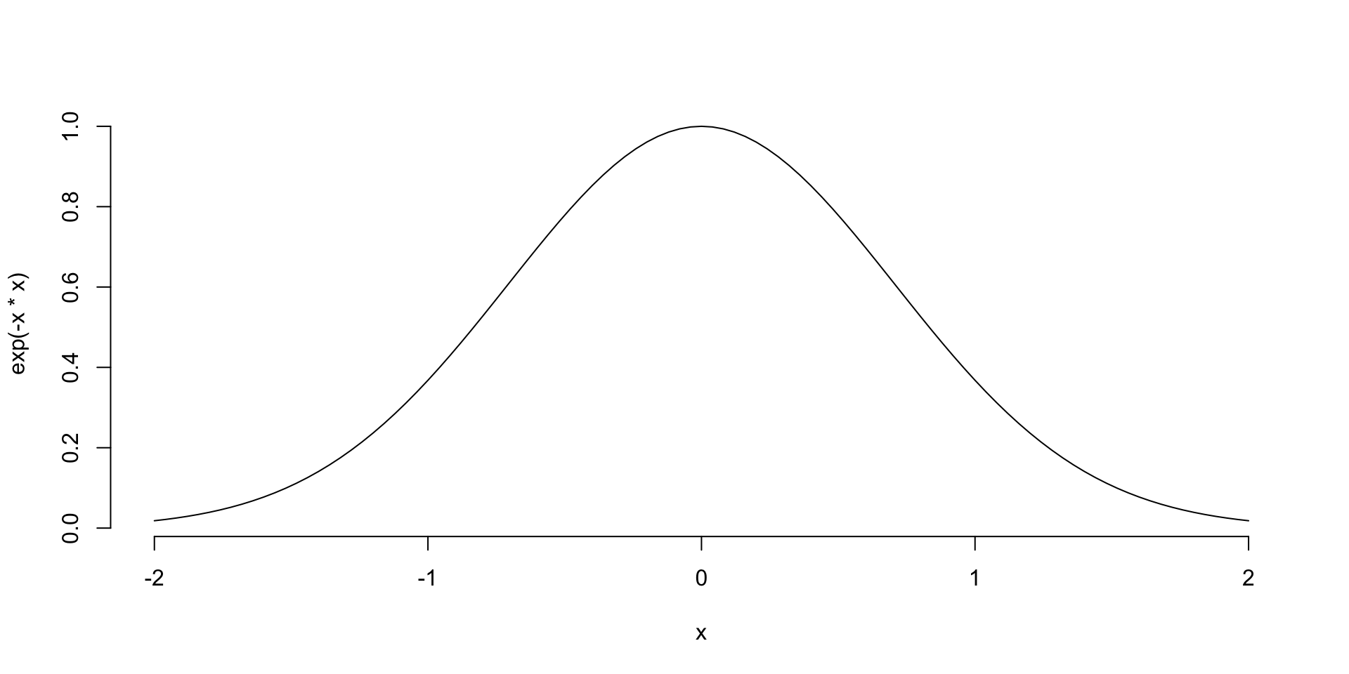
Nonlinear: \(y_t = x_t / (1+ x_t^2) + v_t\)
Simulate Data
Code
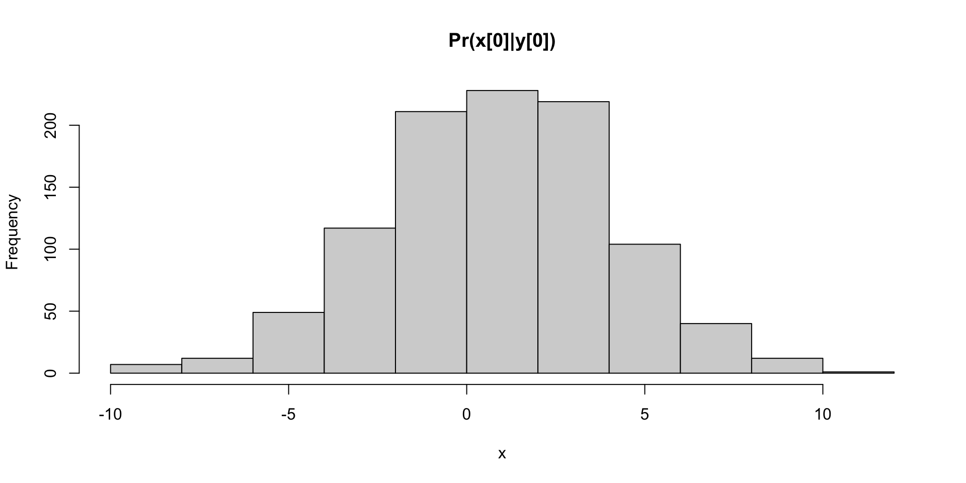
set.seed(8)# MC sample sizeN =1000#Posterior at time t=0 p(x[0]|y[0])=N(1,10)x =rnorm(N,1,sqrt(10))hist(x,main="Pr(x[0]|y[0])")
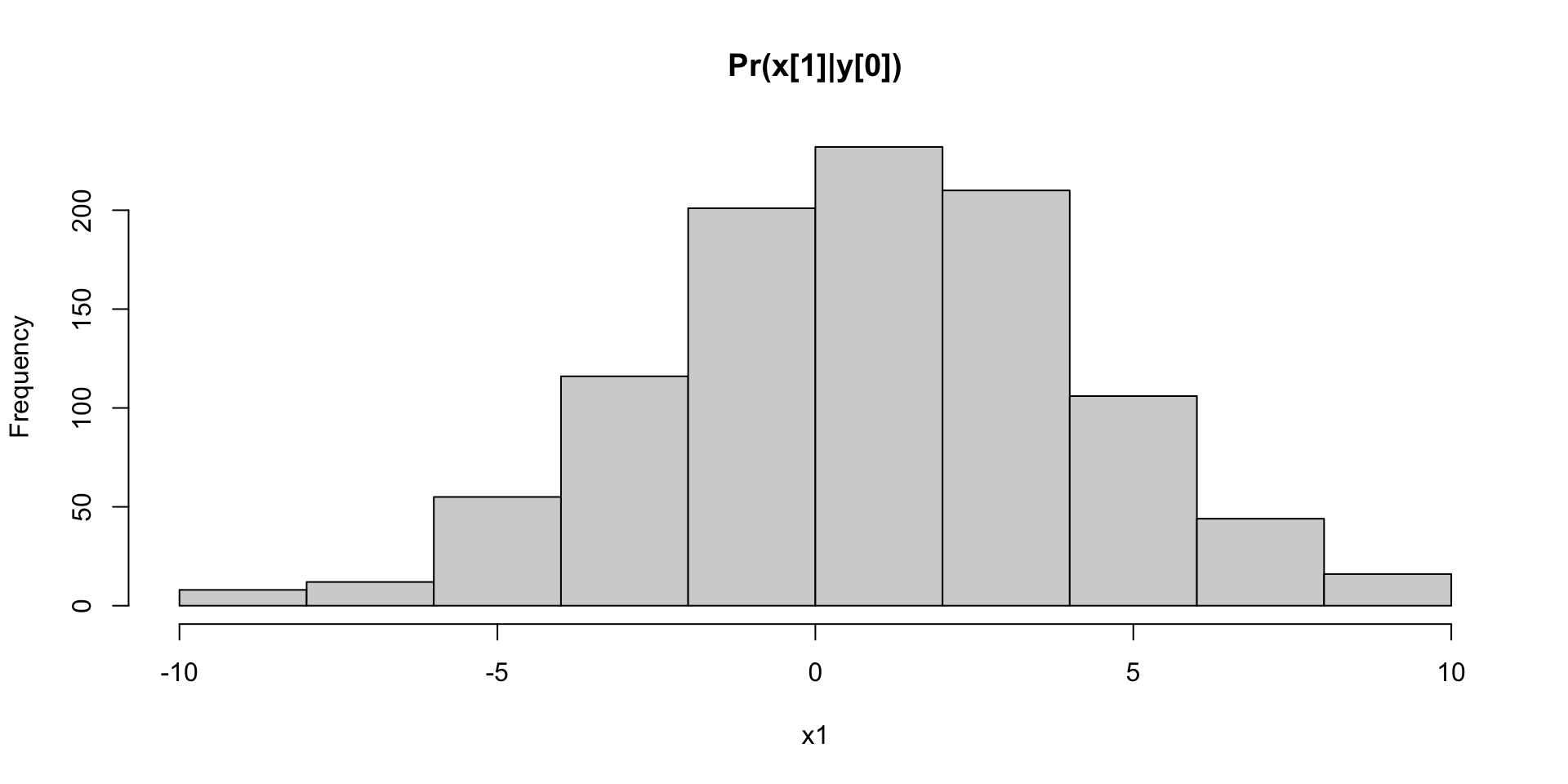
Code
#Obtain draws from prior p(x[1]|y[0])x1 = x +rnorm(N,0,sqrt(0.5))hist(x1,main="Pr(x[1]|y[0])")
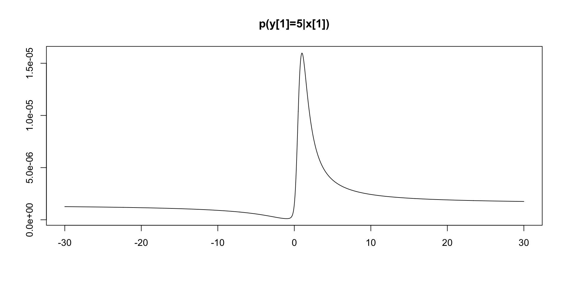
Code
#Likelihood function p(y[1]|x[1])y1 =5ths =seq(-30,30,length=1000)plot(ths,dnorm(y1,ths/(1+ths^2),1),type="l",xlab="",ylab="")title(paste("p(y[1]=",y1,"|x[1])",sep=""))
Nonlinear Filtering
Resampling
Key: resample and propagate particles
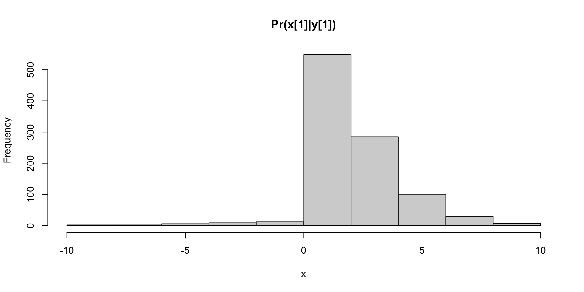
Code
# Computing resampling weightsw =dnorm(y1,x1/(1+x1^2),1)# Resample to obtain draws from p(x[1]|y[1])k =sample(1:N,size=N,replace=TRUE,prob=w)x = x1[k]hist(x,main="Pr(x[1]|y[1])")
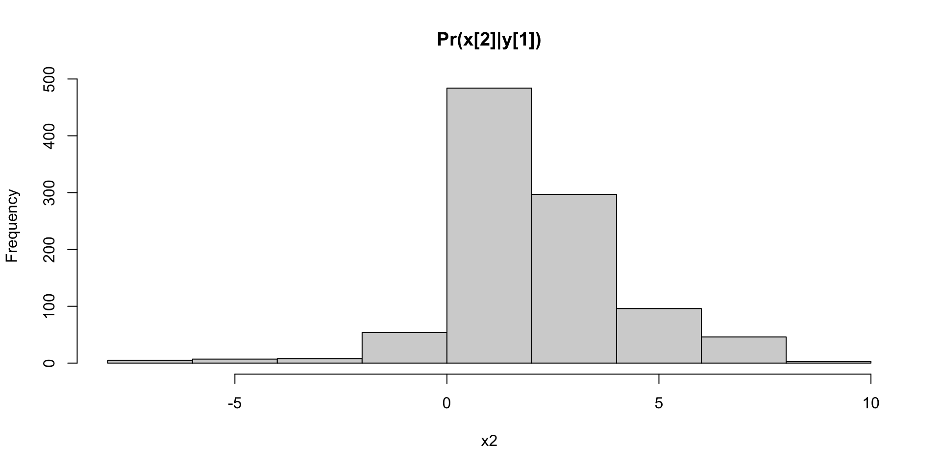
Code
#Obtain draws from prior p(x[2]|y[1])x2 = x +rnorm(N,0,sqrt(0.5))hist(x2,main="Pr(x[2]|y[1])")
Propagation of MC error
Dynamic Linear Model (DLM): Kalman Filter
Kalman filter for linear Gaussian systems
FFBS (Filter Forward Backwards Sample)
This determines the posterior distribution of the states
\[
p( x_t | y^t ) \; {\rm and} \; p( x_t | y^T )
\] Also the joint distribution \(p( x^T | y^T )\) of the hidden states.
Discrete Hidden Markov Model HMM (Baum-Welch, Viterbi)
With parameters known the Kalman filter gives the exact recursions.
Propagate-Resample is replaced by Resample-Propagate
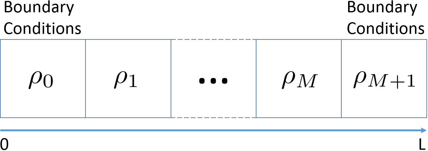
Traffic Problem
State-Space
Wave Speed Propagation is a Mixture Distribution
Shock wave propagation speed is a mixture, when calculated using Godunov scheme \[
w = \frac{q(\rho_l) - q(\rho_r)}{\rho_l-\rho_r} \ \left[\frac{mi}{h}\right] = \left[\frac{veh}{h}\right]\left[\frac{mi}{veh}\right].
\] Assume \(\rho_l \sim TN(32, 16, 0, 320)\) and \(\rho_r \sim TN(48, 16, 0,320)\) \(q_c = 1600 \ veh/h\), \(\rho_c = 40 \ veh/mi\), and \(\rho_{jam} = 320 \ veh/mi\)
Traffic Flow Speed Forecast is a Mixtrue Dsitribution
Theorem: The solution (including numerical) to the LWR model with stochastic initial conditions is a mixture distribution.
A moment based filters such as Kalman Filter or Extended Kalman Filter would not capture the mixture.
Problem at Hand
The Parameter Learning and State Estimation Problem
Goal: given sparse sensor measurements, find the distribution over traffic state and underlying traffic flow parameters \(p(\theta_t, \phi|y_1, y_2,...,y_t); \ \phi=(q_c,\rho_c)\)
Parameters of the evolution equation (LWR) are stochastic
Distribution over state is a mixture
Can’t use moment based filters (KF, EKF,...)
Data Assimilation: State Space Representation
State space formulation allows to combine knowledge from analytical model with the one from field measurements, while taking model and measurement errors into account
Given particles (a.k.a. random draws) \((\theta^{(i)}_t,\phi^{(i)},s^{(i)}_t),\)\(i=1,\ldots,N\)\[
p( \theta_t | y_{1:t} ) = \frac{1}{N} \sum_{i=1}^N \delta_{ \theta^{(i)} } \; .
\]
First resample \((\theta^{k(i)}_t,\phi^{k(i)},s^{k(i)}_t)\) with weights proportional to \(p(y_{t+1}|\theta^{k(i)}_t,\phi^{k(i)})\) and \(s_t^{k(i)}=S(s^{(i)}_t,\theta^{k(i)}_t,y_{t+1})\) and then propogate to \(p(\theta_{t+1}|y_{1:t+1})\) by drawing \(\theta^{(i)}_{t+1}\,\)from \(p(\theta_{t+1}|\theta^{k(i)}_t,\phi^{k(i)},y_{t+1}),\,i=1,\ldots,N\).
Next we update the sufficient statistic as
\[
s_{t+1}=S(s_t^{k(i)},\theta^{(i)}_{t+1},y_{t+1}),
\] for \(i=1,\ldots,N\), which represents a deterministic propogation.
Finally, parameter learning is completed by drawing \(\phi^{(i)}\) using \(p(\phi|s^{(i)}_{t+1})\) for \(i=1,\ldots,N\).
These ingredients then define a particle filtering and learning algorithm for the sequence of joint posterior distributions \(p( \theta_t , \phi | y_{1:t} )\): \[
\begin{aligned}
& \text{Step 1. (Resample) Draw an index } k_t \left( i\right) \sim
Mult_{N}\left( w_{t}^{\left( 1\right) },...,w_{t}^{\left( N\right)
}\right), \\
& \mbox{where the weights are given by } w_t^{(i)} \propto p(y_{t+1}|(\theta_t,\phi)^{(i)}), \ \text{ for }i=1,...,N\\
\text{ } & \text{Step 2. (Propagate) Draw }\theta_{t+1}^{\left( i\right) }\sim
p\left( \theta_{t+1}|\theta_t^{k_t \left( i\right) },y_{t+1}\right) \text{ for
}i=1,...,N.\\
\text{ } & \text{Step 3. (Update) } s_{t+1}^{(i)} =S(s_t^{k_t(i)},\theta_{t+1}^{(i)},y_{t+1})\\
\text{ } & \text{Step 4. (Replenish) } \phi^{(i)} \sim p( \phi | s_{t+1}^{(i)} )
\end{aligned}
\] There are a number of efficiency gains from such an approach, e.g. it does not suffer from degeneracy problems associated with traditional propagate-resample algorithms when \(y_{t+1}\) is an outliers.
Obtaining state estimates from particles
Any estimate of a function \(f(\theta_t)\) can be calculated by discrete-approximation


 Bayes theorem: \[
p(\theta \mid y^t) \propto p(y_t \mid \theta) \,
p(\theta \mid y^{t-1})
\]
Bayes theorem: \[
p(\theta \mid y^t) \propto p(y_t \mid \theta) \,
p(\theta \mid y^{t-1})
\]