12 Adaptive and Bayesian Trial Design
As results accumulate showing one treatment superior, continuing to assign patients equally to both arms becomes progressively more unethical. For most of the 20th century, traditional methodology demanded exactly that. Trials followed a rigid paradigm: fix the sample size in advance, randomize patients equally to treatment and control, analyze the data once at the end, and never peek at accumulating results. The framework was designed to control the probability of false positive conclusions, it succeeded admirably at that goal, and regulators and statisticians understood it well.
It came at a cost. Patients in trials sometimes continued receiving inferior treatments long after the evidence favored the alternative, because the design could not adapt and information accumulating during the trial was deliberately hidden until the very end. Trials that were clearly failing ran to their planned end, and promising drugs took years to reach patients because trials could not accelerate when results were compelling. The methodology prioritized the conclusions drawn after the trial over the welfare of patients during it.
That ordering had a principled defense. The Belmont Report, published in 1979, established the ethical framework for human subjects research in the United States (National Commission for the Protection of Human Subjects of Biomedical and Behavioral Research 1979). It drew a sharp distinction: “The purpose of medical or behavioral practice is to provide diagnosis, preventive treatment or therapy to particular individuals. By contrast, the term ‘research’ designates an activity designed to test an hypothesis, permit conclusions to be drawn, and thereby to develop or contribute to generalizable knowledge.”
This dichotomy shaped clinical trial design for decades. Research was about generalizable knowledge; treatment was about helping patients. The two were separate, and a patient in a clinical trial was participating in science, not necessarily receiving optimal therapy. Treating a patient in a clinical trial should be as important as treating a patient after the trial, yet traditional designs ignored this principle.
The past three decades rethought that paradigm with adaptive designs, Bayesian methods, and platform trials, and this chapter traces that evolution from its theoretical foundations to the trials that established it. The frequentist foundations that rethinking builds on (hypothesis testing, Type I and II error control, survival analysis, repeated-measures models, group-sequential designs, and causal inference methods) are covered in Chapter 11; Berry’s review is a practitioner-oriented synthesis of how the adaptive and Bayesian ideas fit together (D. A. Berry 2025).
12.1 Preliminaries
Chapter 11 opened on Cox’s domain of “large uncontrolled variations,” and everything in this chapter follows from what that variation does to a trial. A patient’s condition fluctuates with the natural history of the disease, with environmental factors, with psychological responses to treatment (the placebo effect), and with the supportive care they receive. Even if every patient in a trial received identical treatment, their outcomes would still vary substantially, and the effect of a new drug is usually a modest improvement over existing therapy that has to be detected against that background. Absolute outcomes say little on their own, which is why trials are built for comparison.
The need for concurrent controls (a group of patients receiving placebo or standard therapy, enrolled in the same trial under the same conditions) follows directly from this logic. It is tempting to compare a new treatment’s results against historical data: “Patients with this disease used to have 30% survival; now with our drug they have 45% survival.” But such comparisons are perilous. Medical practice changes over time. Diagnostic criteria evolve, often detecting disease earlier (lead-time bias). Supportive care improves. Patient populations shift. These “secular changes” can easily produce apparent improvements that have nothing to do with the investigational drug. The classical solution is the concurrent control: with both groups managed under identical conditions, the treatment is the only systematic difference between them.
In the early 20th century, a researcher studying inheritance in rats trained animals to perform a task, then bred from them across multiple generations, measuring how quickly each generation learned the task. He observed steady improvement across generations, apparently supporting a theory that acquired traits could be inherited. But there were no controls: no rats bred under identical conditions from untrained parents. When other researchers repeated the experiment with controls, they found that both trained and untrained lineages showed the same improvement over time. The apparent effect was due to secular changes in the health of the rat colony, not inherited learning. Without concurrent controls, this confounding factor was invisible.
Unless a treatment effect is dramatic (what statisticians sometimes call a “penicillin effect,” where the improvement is so large it overwhelms any background variation), the comparison must be made against concurrent controls. Except in rare circumstances (such as diseases with 100% mortality and no existing treatment), historical controls cannot provide the certainty needed for regulatory approval.
The structure of a clinical trial follows from its comparative nature. Patients are assigned to treatment arms (the groups being compared). The investigational arm receives the new therapy being tested. The control arm receives either a placebo (an inactive substance designed to be indistinguishable from the active drug) or an active control (the current standard-of-care treatment). The endpoint is the outcome measured to determine whether the treatment worked, for example, survival time, tumor shrinkage, or improvement on a symptom scale. The treatment effect is what we are trying to estimate: the true difference in outcomes between the investigational arm and the control arm.
The population is everyone with the condition of interest, all the people who might eventually receive the drug if approved. The sample is the much smaller subset actually enrolled in the trial. Because we can only study a sample, our conclusions about the population are always uncertain, and that uncertainty is quantified using probability, a number between 0 and 1 (or equivalently, 0% to 100%) running from impossible to certain.
Efficacy is the treatment’s ability to produce the desired beneficial effect under the controlled conditions of a trial. Effectiveness is how well it works in routine clinical practice, where patients may be older, sicker, or less adherent to the prescribed regimen than those carefully selected for a trial.
A valid clinical trial must satisfy five requirements.
Absence of systematic error (bias). Patients receiving different treatments must not differ systematically in ways that could affect outcomes. If healthier patients are assigned to the investigational arm and sicker patients to the control arm, any observed benefit might be due to patient selection rather than the drug. The difficulty is that such bias cannot be removed by statistical analysis after the fact. No calculation of statistical significance can distinguish a treatment effect from a confounding factor: a small p-value says only that the observed difference would be surprising if chance alone were at work, not what produced it.
The solution is randomization: using a chance mechanism (like a computer-generated random number) to assign each patient to a treatment arm (Cox 2009). (For practical implementation of randomization methods, see Chapter 16.) Randomization serves three purposes: it avoids selection and other biases in a publicly convincing way; it provides a unified basis for estimating statistical error across different trial designs; and it enables formally exact tests of significance. Of these, bias avoidance is largely uncontroversial: randomization ensures that any differences between groups, whether known factors like age and disease severity or unknown factors we have not even thought to measure, are distributed randomly rather than systematically. This allows us to attribute observed differences to the treatment itself with quantifiable confidence.
A related principle: the units assigned to each treatment must respond independently of one another. If all patients receiving the new drug are treated at one hospital and all control patients at another, we cannot separate the drug effect from differences between hospitals: the hospital has become the experimental unit, and each arm has only one. The remedy is to randomize patients within each site or, when the intervention acts on a whole site, to randomize many sites and account for the clustering in the analysis (see Chapter 13).
Precision. Even when systematic error is eliminated through randomization, our estimate of the treatment effect will differ from its true value due to random error (the natural fluctuation that occurs when studying a sample rather than the entire population). The standard error measures the expected magnitude of this random error. A rough interpretation: in about one case out of three, the estimate will err by more than \(\pm 1\) standard error; in about one case out of twenty, by more than \(\pm 2\) standard errors; in about one case out of a hundred, by more than \(\pm 2.6\) standard errors.
The standard error follows a square-root law: it is proportional to \(1/\sqrt{n}\), where \(n\) is the number of patients per treatment arm (the drug group, placebo group, etc.). To halve the standard error (to double the precision of our estimate) we must quadruple the number of patients in each arm; to reduce it by a factor of ten requires a hundredfold increase in patients. Precision is costly, which is why confirmatory trials (the large Phase III studies required for regulatory approval) are so expensive, and why improved trial design (using techniques like stratification or crossover to reduce variability) can be more efficient than simply enrolling more patients.
Range of validity. The conclusions drawn from a trial strictly apply only to the specific patients and conditions studied. How well the trial’s design and conduct protect those conclusions from bias is its internal validity. But the scientific and public health value of a trial depends on external validity (also called generalizability): the extent to which findings can be extrapolated to broader patient populations.
The two are in tension. A trial restricted to young, otherwise healthy patients will have less outcome variability and therefore require fewer subjects to achieve a given precision, but its results may not apply to elderly patients with multiple conditions, the very patients who will receive the drug in routine practice. Broad enrollment criteria reverse the trade: more generalizable results, more patients needed for the same precision because outcomes are more variable.
Simplicity. The trial should be as simple as practical. Complex protocols with frequent treatment changes are difficult for research staff to execute correctly, and operational difficulties can compromise data quality. Nevertheless, some complexity may be advantageous (adaptive designs that modify treatment assignments based on accumulating data, for instance), and it is a matter of judgment how far to go.
Quantifiable uncertainty. It must be possible to calculate the uncertainty in the conclusions, ideally from the trial data themselves. Statistical analysis provides both: an estimate of the treatment effect, and a measure of how confident we can be in it. The use of randomization to eliminate systematic differences automatically makes remaining differences random, which justifies the statistical analysis under weak assumptions.
These five requirements are met, in conventional practice, by the frequentist machinery set out in Chapter 11: the null hypothesis and the p-value, Type I and Type II error, power, and a sample size fixed in advance from the minimum clinically important difference. That chapter also covers the intent-to-treat principle and the ICH E9(R1) estimands framework that now sits alongside it. The name is apt, since the framework reads probability as the frequency of outcomes over many repeated trials, and it has governed regulatory decision-making for decades. What matters here is its shape rather than its details. It does not answer the question sponsors and regulators actually ask, which is how probable it is that this drug works given the data. It answers how improbable the data would be if the drug did nothing.
The framework is rigid by design. Sample size is calculated before the trial begins based on assumptions about the treatment effect, variability, desired power, and acceptable Type I error, and once the trial starts those parameters are fixed. Looking at accumulating data and deciding to enroll more patients if results are borderline (a natural impulse) inflates the Type I error rate; stopping early when results look promising, without pre-specified rules, does the same. The price of controlling error rates is inflexibility.
Abraham Wald laid the mathematical foundations for analyzing sequential decisions with the Sequential Probability Ratio Test, developed during World War II for industrial quality control (Wald 1947), and Albert Shiryaev later formalized them in optimal stopping theory (Shiryaev 1978). Peter Armitage recognized in 1954 that these methods could address an ethical tension in clinical trials (Armitage 1954, 1960): if one treatment is clearly superior, continuing to randomize patients to the inferior arm is unjustifiable. Sequential methods allow trials to stop early while maintaining valid statistical inference, but they require the stopping rules to be specified in advance.
When traditional designs break down. The five requirements for a valid trial (absence of bias, precision, range of validity, simplicity, and quantifiable uncertainty) were developed in an era of relatively homogeneous patient populations and treatments with broad applicability. Modern medicine increasingly operates in a different world (D. A. Berry 2012), and regulators have responded with new guidance frameworks.
A drug may work extraordinarily well in 15% of patients who carry a particular genetic mutation and have no effect in the other 85% who lack it. That pattern is the premise of precision medicine (also called personalized medicine), where treatments are targeted to patients with specific characteristics (U.S. Food and Drug Administration 2019c; Zhou et al. 2008). The characteristic that marks out the responders is a biomarker, a measurable biological indicator (such as a genetic mutation, a protein level in the blood, or a molecular characteristic of a tumor) that can predict whether a patient will respond to a particular treatment. The traditional framework (randomize patients equally, analyze the average treatment effect across all patients) will dramatically underestimate the benefit for the responsive subgroup while exposing non-responders to ineffective treatment.
The FDA’s enrichment strategies guidance addresses this challenge by describing predictive enrichment (selecting patients likely to respond based on biomarker status) and prognostic enrichment (selecting patients at higher risk of the outcome), but these approaches create new tensions. The “range of validity” requirement becomes paradoxical: a trial enrolling all patients has broad generalizability but may miss a genuine effect in the responsive subgroup; a trial restricted to biomarker-positive patients (those with the predictive characteristic) may have insufficient patients for adequate precision. Adaptive enrichment designs address this by starting with broad enrollment and using interim data to identify responsive subgroups, restricting subsequent enrollment accordingly (Simon and Simon 2013; Pallmann et al. 2018). Recent advances in covariate-adaptive randomization allow trials to balance treatment assignments across patient characteristics more efficiently, with unified frameworks that can handle continuous covariates and complex covariate structures (Atkinson 2002; Ma et al. 2024).
Rare diseases present an even starker challenge (European Medicines Agency 2006; U.S. Food and Drug Administration 2025). If only 5,000 patients worldwide have a condition, enrolling 1,000 patients for a Phase III trial (a modest size for common diseases) would require recruiting 20% of the entire patient population. The square-root law governing precision becomes an insurmountable barrier: there simply are not enough patients to achieve traditional power levels for modest effect sizes. Recognizing this, regulators have developed more flexible ways to meet the existing evidentiary standard. Under the FDA’s proposed Rare Disease Evidence Principles (RDEP) process, one adequate and well-controlled study, possibly single-arm, plus strong confirmatory evidence can generally establish effectiveness; the process is limited to drugs for a known inborn genetic defect in a very small population (generally fewer than 1,000 U.S. patients) whose disease progresses to significant disability or death in a relatively short time and has no adequate therapy that alters its course. The EMA’s guideline on small populations explicitly addresses alternative study designs including non-randomized approaches and external controls.
Multiple treatment options compound the difficulty (U.S. Food and Drug Administration 2022; Redman et al. 2020; Renfro and Sargent 2017). Modern oncology trials may need to evaluate several drugs, each potentially combined with several others, across multiple biomarker-defined subgroups. A traditional approach (separate trials for each combination in each subgroup) would take decades and hundreds of thousands of patients. The requirement for “simplicity” becomes impossible when the clinical reality is inherently complex. The FDA’s master protocols guidance describes innovative designs: basket trials (studying one drug across multiple tumor types sharing a biomarker), umbrella trials (studying multiple drugs within one tumor type based on biomarkers), and platform trials (flexible frameworks that can add or remove treatment arms over time). All three put multiple treatments or multiple patient populations inside a single trial infrastructure.
In these settings the traditional design (fixed sample size, equal randomization, single analysis at the end) is not merely suboptimal. It is potentially unethical or infeasible. Continuing to randomize patients equally to a clearly inferior arm wastes their contribution. Conducting underpowered trials (trials with too few patients to reliably detect a true treatment effect) in rare diseases wastes resources and patient willingness to participate, and testing one combination at a time when patients are dying delays potentially life-saving treatments for years.
The case for adaptive designs. These challenges have driven the development of adaptive trial designs (trials that modify themselves based on accumulating data according to pre-specified rules) (S. M. Berry et al. 2010). Instead of fixing everything before the first patient enrolls, an adaptive design lets the trial learn and adjust. Two oncology programs show what that buys: the BATTLE trial used Bayesian adaptive randomization to match lung cancer patients to targeted therapies based on their tumor biomarkers (Kim et al. 2011), and the I-SPY 2 platform trial has evaluated more than twenty neoadjuvant breast cancer treatments, graduating effective drugs to Phase III while dropping ineffective ones (Wang and Yee 2019).
The rigidity of traditional designs is not inherent to valid inference. If we can pre-specify the rules by which adaptations will occur (writing them into the protocol before the trial begins) and use computer simulations to verify that the trial still controls Type I error under various scenarios, we can maintain regulatory standards while gaining flexibility. The adaptation rules become part of the design, not modifications made after seeing the data.
Adaptive designs can drop ineffective treatment arms early, concentrating resources on promising therapies, and can shift randomization toward better-performing treatments, reducing the number of patients assigned to inferior arms. Sample size can rise if interim results (analyses conducted partway through the trial, before all patients have completed) suggest the treatment effect is smaller than anticipated. And where the drug works best in a subgroup defined by biomarkers, the design can find it.
A complementary approach uses Bayesian statistical methods, which directly answer the question the frequentist framework does not: “Given the data we have observed, what is the probability that this drug works?” Bayesian methods naturally accommodate accumulating evidence, updating probability estimates as each new patient’s data arrives, making them well-suited for adaptive designs. They also provide a coherent framework for borrowing information (using data from previous trials, from other patient subgroups, or from external sources to supplement the current trial’s data), which is especially valuable in rare diseases where every patient’s data is precious.
Chapter 30 provides definitions of key terms used throughout this chapter.
12.2 Bandit Problems: The Theoretical Foundation
In 1933, statistician W.R. Thompson proposed a radical idea (Thompson 1933). When testing two treatments with unknown efficacy, assign the next patient to treatment A with probability equal to the current probability that A is better than B. Thompson was motivated by ethics: avoiding patients being “sacrificed to the inferior treatment.” His proposal predated Austin Bradford Hill’s first randomized controlled trial by 15 years.
Thompson had discovered what mathematicians would later call a multi-armed bandit problem, a fundamental challenge in decision theory. Imagine slot machines (bandits) with unknown payout rates. You want to maximize total winnings over many pulls. Each pull gives information (which machine pays better?) and potentially gives a reward (you might win). The dilemma: should you exploit by playing the machine that seems best, or explore by trying other machines to learn more? This is the exploration-exploitation tradeoff.
Clinical trials are bandit problems. Each patient assignment is a “pull.” Some pulls give information about treatment efficacy (explore). Some give effective therapy to the patient (exploit). The goal is maximizing successful outcomes across all patients, both those in the trial and those who will be treated after the trial based on its results. The challenges that break traditional designs (precision medicine, rare diseases, multiple treatment options) are instances of this structure, and its formal study provides the theoretical foundation for adaptive trial designs.
Early statisticians recognized that fixed randomization (ignoring accumulating data) was clearly suboptimal. If you know which treatment works better, use it. But in trials, you don’t know; you learn as you go. The question becomes: what strategy adapts optimally as evidence accumulates?
Finding the mathematically optimal strategy is computationally demanding, and the difficulty grows explosively as the number of arms and the length of the trial increase. For a small number of arms, though, the optimal strategy can still be computed exactly through dynamic programming, working backward from the last patient. For patient N, the decision is easy: choose whichever arm has higher probability of success. For patient N-1, choose the arm that maximizes expected total successes for the last two patients, accounting for what will be learned. Work backward to patient 1.
Consider testing two treatments with unknown success rates in four patients. Starting with uniform prior beliefs (complete uncertainty about both treatments), an optimal adaptive strategy achieves an expected success rate of 56.9%, compared to 50% for any fixed randomization scheme. The benefit grows with sample size: at 100 patients, the adaptive strategy reaches 64.9%; with infinite patients, it approaches 66.7%, a 16.7 percentage point gain representing the expected value of perfect information.
Thompson’s strategy turns out to be effective in practice, especially when testing many treatments simultaneously. It is not mathematically optimal, but it is intuitive and it performs well. After 70 years of obscurity, Thompson’s 1933 paper has seen explosive growth in citations, driven by applications ranging from search engine ad placement to modern platform trials.
Bayesian Bandit Problems: Updating Beliefs
The mathematical foundation of bandit problems rests on Bayesian updating, the process of revising probability distributions as evidence accumulates (D. A. Berry 2025). Consider a simple two-armed trial where both treatments have unknown success probabilities \(p_1\) and \(p_2\). Before observing any data, we might assume complete uncertainty: both success rates follow uniform distributions on [0, 1], which is equivalent to a Beta(1, 1) distribution.
As outcomes are observed, beliefs update according to Bayes’ rule:
\[ P(\theta|D) = \frac{P(D|\theta)P(\theta)}{P(D)} \]
For a binary outcome (success/failure), if a treatment produces \(s\) successes and \(f\) failures, and we start with a Beta(1,1) prior, the posterior distribution for its success rate \(p\) becomes Beta(\(\alpha_{post}, \beta_{post}\)), where:
\[ \alpha_{post} = 1 + s, \quad \beta_{post} = 1 + f \]
The posterior mean, representing our updated best estimate of the success rate, is given by \(\frac{\alpha_{post}}{\alpha_{post} + \beta_{post}}\), and the variance, representing our uncertainty, is \(\frac{\alpha_{post}\beta_{post}}{(\alpha_{post}+\beta_{post})^2 (\alpha_{post}+\beta_{post}+1)}\). This elegant conjugacy enables exact updating without numerical approximation.
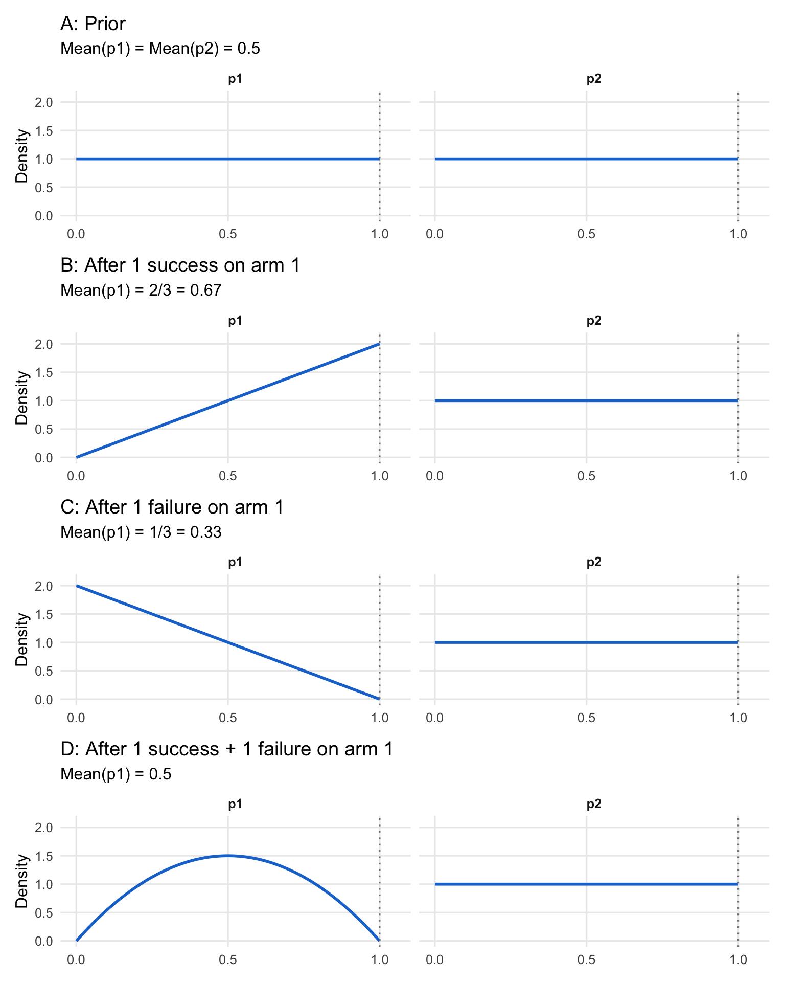
Figure 12.1 illustrates this updating process for a four-patient bandit problem, showing how the probability distribution for \(p_1\) evolves while \(p_2\) (with no observations yet) remains uniform:
With uniform priors, a single success shifts the mean from 0.5 to 2/3, while a failure shifts it to 1/3. After one success and one failure, the mean returns to 0.5, but the distribution is no longer uniform. It is now peaked at 0.5 with less variance, reflecting the additional information that the true rate is unlikely to be extreme.
Despite the elegant theory, Bayesian adaptive trials remained curiosities for decades. Biostatisticians in the 1970s and 1980s considered them naive: randomization was sacrosanct, the gold standard of medical research, and varying randomization probabilities based on accumulating data was viewed with deep suspicion.
One investigator remarked that Bayesians were “loosey-goosey” in adhering to rules. The concern was legitimate: if you look at data repeatedly and adjust your trial, don’t you inflate Type I error? Can such trials be trusted?
The path forward ran through traditional trial design: demonstrate mastery of it first, gain credibility in the clinical research community, then introduce innovations incrementally. It also took advances in computing power and statistical software to make complex calculations feasible, and regulators willing to embrace innovation while maintaining rigorous standards.
By the late 1990s, these pieces were falling into place. The FDA’s Center for Devices and Radiological Health (CDRH) led early adoption, commissioning white papers on Bayesian approaches in medical device development. Early successes in late-phase device trials demonstrated that Bayesian methods could work in practice, maintaining control of Type I error while providing decision-makers with more intuitive, actionable information.
12.3 The First Wave of Bayesian Adaptive Trials: Proving the Concept
The first wave of real-world Bayesian adaptive trials (late 1990s through the 2010s) did not set out to replace frequentist practice. They succeeded by embedding Bayesian quantities inside conservative, auditable decision rules that stakeholders already understood: stop or continue enrollment, drop unpromising doses, or graduate a regimen to confirmatory testing. The common thread is operational: these designs turned interim data into actionable forecasts (especially predictive probabilities) while still demonstrating familiar operating characteristics through simulation and error-rate control. The examples below became proof points because they were clinically consequential, computationally feasible, and easy to explain to sponsors and regulators in plain language.
CALGB 49907: Predicting Trial Outcomes
In 1999, a fully Bayesian trial was designed for the Cancer and Leukemia Group B (CALGB) testing whether capecitabine could replace standard chemotherapy in elderly breast cancer patients (Muss et al. 2009). The sponsor insisted on 1800 patients to answer the question adequately. The statistical team estimated this would take 15 years to accrue, by which time the question might no longer be interesting.
The compromise: enroll 1800 patients only if needed. Starting at 600 patients, calculate Bayesian predictive probabilities: given current data, what is the probability that further follow-up (without additional enrollment) will answer the question conclusively? If this probability exceeds 80%, stop enrollment and continue follow-up.
The trial stopped at the first interim analysis with 633 patients enrolled. Additional 16-month follow-up delivered a compelling answer: capecitabine cannot replace chemotherapy in this population. The trial achieved its scientific goal with one-third the planned sample size.
By Berry’s account, this was the first fully Bayesian randomized trial published in the New England Journal of Medicine (2009). It demonstrated a key principle: predictive probabilities answer the question sponsors and clinicians actually care about (“Will this trial give us a definitive answer?”) more directly than traditional power calculations.
ASTIN: Adaptive Dose-Finding in Stroke
Pfizer’s ASTIN trial (Acute Stroke Therapy by Inhibition of Neutrophils) tested 15 doses plus placebo of an investigational neutrophil inhibitor in stroke patients (Krams et al. 2003). Allocation probabilities were never fixed upfront. The trial analyzed data daily and used Bayesian modeling to decide which doses to assign the next day.
The algorithm smoothed estimates across doses and used longitudinal models to predict 90-day outcomes from earlier measurements. It began on low doses and placebo, saw little effect, and progressively concentrated on higher doses as evidence accumulated. By the time 500 patients had completed 90-day follow-up, it had concluded the drug was ineffective at every dose and stopped the trial, which randomized 966 patients, well short of the 1300 maximum.
This was dose-finding as a bandit problem: continuously learning which doses were most promising and concentrating resources there, while exploring enough to avoid missing an effective dose.
12.4 Seamless Designs: Combining Phases
Phase II and Phase III decisions are traditionally separated by years and by organizational boundaries: one study ends, a fresh protocol is written, a new trial starts. Seamless Phase II/III designs collapse that gap. Interim learning (often supported by Bayesian modeling and predictive thinking) selects doses or regimens early, and accrual continues into a confirmatory stage under prespecified rules. The motivation is economic and ethical. Cutting the “dead time” between phases delivers decision-grade evidence sooner without sacrificing interpretability, and choosing doses from the trial’s own interim data avoids overcommitting to a weak one.
AWARD-5: From Seven Doses to Blockbuster Drug
Eli Lilly’s AWARD-5 trial for dulaglutide (Trulicity) in type 2 diabetes began in 2008 with seven doses (0.25 to 3.0 mg) plus two controls, designed in collaboration with the FDA as part of the Critical Path Initiative (D. A. Berry 2025). Stage 1 used response-adaptive randomization with biweekly interim analyses, scored by a composite clinical utility index that combined HbA1c, weight loss, heart rate, and blood pressure, capturing both efficacy and safety in a single metric.
Longitudinal modeling predicted 12-month outcomes from early data, so doses could be selected before any patient reached the primary endpoint. The algorithm picked two non-adjacent doses (0.75 and 1.50 mg) at the earliest allowed timepoint and shifted directly to Stage 2: fixed randomization comparing those doses to controls.
The Data Safety Monitoring Board could depart from the algorithm only on matters of safety (D. A. Berry 2025), and on those grounds, in April 2009, randomization to the 3.0 mg dose was stopped on its recommendation after increases in heart rate and concerns about pancreatic safety (European Medicines Agency 2014). Its members remarked that they could not otherwise overrule the algorithm’s decisions, but that if they could, they would do exactly what the algorithm had done.
Both doses received FDA approval in 2014. Trulicity became Lilly’s best-selling drug, reaching peak annual revenue of $7.4 billion in 2022 according to Lilly’s financial reporting, and, by Berry’s estimate, the seamless design saved at least one year compared to running separate Phase II and III trials (D. A. Berry 2025). The 3.0 mg dose, though dropped in Stage 1, showed a mean weight loss of 3.3 kg (about 7 pounds) in the 15 patients randomized to it, against about 0.5 kg on the control arms, in data up to the dose-selection point (European Medicines Agency 2014). That signal foreshadowed the modern use of GLP-1 agonists for obesity, even though Trulicity itself was never approved for weight loss.
Lecanemab: From Adaptive Phase II to Phase III
When Eisai designed their Phase II trial (Study 201) for lecanemab (Leqembi) in Alzheimer’s disease in 2011, they aimed to avoid a common failure mode: Phase II trials that give false signals, leading to failed Phase III trials (Swanson et al. 2021; Dyck et al. 2023; D. A. Berry 2025).
The trial tested six dose regimens including placebo. Initially, 2/7 of patients were randomized to placebo and 1/7 to each dose; at interim analyses after the first 196 patients and then after every 50 more, up to about 800 (Swanson et al. 2021), the proportion assigned to placebo was adjusted to match the proportion for the most likely Phase III dose. Early data favored the highest doses, and by trial end 48% of patients had received the two highest doses while only 12% received the two lowest. The trial was maximally informative about the regimens of greatest interest.
Berry describes missing data above 30% as typical of Alzheimer’s trials. By his account, traditional “last observation carried forward” (LOCF) imputation would have estimated only a 13% reduction in disease progression, probably insufficient to justify Phase III. Bayesian multiple imputation, prospectively specified, learned patterns of missingness: it attributed placebo dropouts largely to the treatment not working, while dropouts on the highest dose were mostly due to a regulatory mandate unrelated to efficacy. The Bayesian model estimated a 27% reduction (D. A. Berry 2025).
Eisai proceeded to Phase III. The confirmatory trial showed 27% less decline than placebo on its primary endpoint, the CDR-SB (Dyck et al. 2023). The match is less exact than it looks: the Phase II 27% was on ADCOMS, and the Phase II Bayesian estimate on the CDR-SB was 33% (Swanson et al. 2021). Both are point estimates with uncertainty, but the Phase II estimates were accurate enough to right-size the Phase III (D. A. Berry 2025). The FDA granted accelerated approval, then full approval, and lecanemab became the first disease-modifying therapy for Alzheimer’s disease with clear efficacy evidence.
12.5 Platform Trials
A platform trial is standing infrastructure. Therapies enter and exit over time against a shared control arm, Bayesian hierarchical models can support learning across biomarker-defined subgroups, and pre-specified decision thresholds control false positives. The obvious benefit is efficiency, since a shared control arm reduces redundant randomization. The subtler one is continuity: evidence accumulates in a coherent framework across calendar time while the operational machinery (data pipelines, governance, DSMB processes, endpoint adjudication) stays stable.
I-SPY 2: Prototype for a New Paradigm
From 2010 to 2022, the I-SPY 2 platform in neoadjuvant breast cancer cycled 23 investigational therapies from 18 pharmaceutical companies through a single trial engine (Park et al. 2016; D. A. Berry 2025). Nine graduated to Phase III on a high Bayesian predictive probability of success (\(\geq 85\%\) probability of success in a confirmatory trial). Four have received FDA marketing approval.
Patients were classified into eight molecular subtypes based on hormone receptor status, HER2 status, and genomic markers. Each experimental therapy was evaluated within relevant subtypes, up to ten possible “signatures” (potential regulatory indications). The trial used response-adaptive randomization, assigning 20% to control (or 50% if only one experimental arm was available) and distributing the remainder based on performance.
A common control arm, pooling concurrently randomized patients with historical controls through a “time machine” approach, gave I-SPY 2 a control cohort an order of magnitude larger than a traditional Phase II study. Around it, monthly continuous learning updated probability distributions across all arms and subtypes; longitudinal modeling used tumor volume measurements to predict pathologic complete response well before patients reached their final assessments; and nested factorials within the continuing control arms tested combination therapies simultaneously, isolating the effects of individual components more efficiently than separate trials would permit.
Neratinib graduated in the HER2-positive, hormone-receptor-negative signature. Across all 115 patients assigned to neratinib, pCR rate was 37% versus 20% for controls, a 17% absolute difference. Berry’s modeling decomposed that gap (D. A. Berry 2025): 7% was the drug’s inherent efficacy, and 10% was due to adaptive randomization concentrating assignments in responsive subtypes. Patients in I-SPY 2 were therefore participating in rigorous research and receiving optimized therapy at the same time. The Belmont Report itself allows research and practice to be “carried on together,” provided the activity undergoes review for the protection of human subjects (National Commission for the Protection of Human Subjects of Biomedical and Behavioral Research 1979).
Building on BATTLE, the Bayesian adaptive lung-cancer master protocol that accrued from 2006 to 2009, I-SPY 2 in turn served as prototype for platform trials across diseases: GBM AGILE in glioblastoma, REMAP-CAP in community-acquired pneumonia (which proved critical during COVID-19), and Precision Promise in pancreatic cancer.
The Regulatory Evolution
In 2010, FDA’s draft guidance allowed that a Bayesian approach to modeling and simulation “might be useful,” then added a caution: “Using simulations to demonstrate control of the Type I error rate, however, is controversial and not fully understood” (U.S. Food and Drug Administration 2010; D. A. Berry 2025). By 2019, the agency had accepted the approach (U.S. Food and Drug Administration 2019a): “The guidance also advises sponsors on the types of information to submit to facilitate FDA evaluation of clinical trials with adaptive designs, including Bayesian adaptive and complex trials that rely on computer simulations for their design.”
The 2019 guidance addressed practical issues like post-simulation: if operating characteristics were evaluated under certain assumptions (e.g., expected accrual rates) but the trial experienced different conditions, additional simulations after the trial could verify that conclusions remain valid.
The FDA’s January 2026 draft guidance on Bayesian methodology in clinical trials (https://www.fda.gov/media/190505/download) spells out what the agency expects when Bayesian methods appear in a submission: Bayesian success criteria and decision thresholds prespecified, operating characteristics evaluated (often through simulation), prior distributions carefully justified (especially when they borrow external information), and sensitivity analyses planned that examine prior-data conflict and other key assumptions. It also stresses documentation and reporting practices sufficient for regulatory review and reproducibility, including clear statements of what was prespecified and how computation was performed (U.S. Food and Drug Administration 2026b).
Its operational value is that it turns Bayesian “acceptability” into reviewable components instead of a broad philosophical debate. A sponsor must be able to show how the decision rule maps to error control and interpretability, how prior influence is understood and bounded (including concepts such as effective sample size and discounting when borrowing), how estimands and missing data are treated in a Bayesian setting, and how results can be reproduced, which means software reliability and, when relevant, convergence diagnostics for simulation-based inference (U.S. Food and Drug Administration 2026b).
The draft ICH E20 guideline on adaptive clinical trials adds international harmonization, though its scope centers on pre-specification, simulation-based demonstration of operating characteristics, and Type I error control, and does not reach the full range of Bayesian adaptive applications the FDA Bayesian guidance covers (International Council for Harmonisation 2025).
ICH E20 and some regulatory commentary have framed Bayesian adaptive trials primarily in terms of borrowing from external data using informative priors. Many Bayesian adaptive trials use minimally informative priors that are rapidly overwhelmed by accumulating data; the benefits come from the coherent inferential framework and from the interpretability of decision rules based on posterior and predictive probabilities (U.S. Food and Drug Administration 2019a). Modern Bayesian borrowing, where it does occur, employs dynamic approaches in which the degree of borrowing depends on observed consistency between external and new data, reducing the bias risk of static borrowing. The Bayesian framework is well suited for sophisticated borrowing, but borrowing and Bayesian analysis are conceptually separate (International Council for Harmonisation 2025).
The One-Trial Standard
FDA has grown increasingly open to accepting a single highly stringent trial as substantial evidence of efficacy in place of two independent Phase III trials (U.S. Food and Drug Administration 2019b; United States Congress 1997). The 1997 modernization act codified the exception, and the agency’s 2019 guidance describes what strengthens the case for a single trial: a hard clinical endpoint, a substantially lower p-value threshold than the conventional two-trial 0.025, large multicenter enrollment, and internal consistency across pre-specified subgroups. In June 2026, FDA issued a revised draft guidance that repositions the single-trial-plus-confirmatory-evidence approach from a bounded exception toward what FDA’s leadership calls the default (Prasad and Makary 2026) and drops the earlier framing that treated one such trial as equivalent to two; because it remains a draft (the public comment period closed on September 22, 2026), it signals regulatory direction rather than settled policy (U.S. Food and Drug Administration 2026a) (see Section 29.7).
The shift fits adaptive designs. A seamless Phase II/III trial with extremely conservative success criteria could deliver both dose optimization and confirmatory evidence in one study, saving years of development time.
It carries costs too. Approvals tied to narrowly defined populations may restrict labeled indications, leaving clinicians to extrapolate off-label or sponsors to run “label expansion” trials after approval. The change could accelerate time to market while shifting weight onto post-approval research and multi-cohort basket architectures.
The optimal evidence standard should arguably depend on context: disease severity, unmet medical need, and patient impact. For fatal rare diseases, a more flexible bar may be justified; for high-prevalence, lower-risk conditions, standards should be stricter. Context-varying standards are good science and hard to implement in regulation.
When Lilly’s AWARD-5 data were presented, when device trials using Bayesian predictive probabilities supported marketing approvals, when I-SPY 2 demonstrated that adaptive trials could maintain scientific rigor while improving patient care, resistance gave way to acceptance.
12.6 Mathematical Foundations: Hierarchical Modeling
Modern adaptive trials often employ Bayesian hierarchical models (probability distributions of probability distributions), which are well suited to basket trials testing one therapy across multiple tumor types and to platform trials testing multiple therapies across patient subtypes (D. A. Berry 2025).
Consider a therapy tested in \(K\) tumor types. For each type \(k\), let \(\theta_k\) denote the true response rate. A hierarchical model specifies:
\[ \theta_k \sim \text{Beta}(\alpha, \beta) \quad \text{for } k = 1, \ldots, K \]
where \(\alpha\) and \(\beta\) are themselves unknown parameters with their own prior distributions (hyperpriors). If we observe \(y_k\) responders out of \(n_k\) patients in tumor type \(k\), the likelihood is:
\[ y_k \mid \theta_k \sim \text{Binomial}(n_k, \theta_k) \]
Through the shared hyperparameters, the data from every tumor type inform the posterior for each \(\theta_k\). If nine types show 40% response rates and one shows 10%, a typical hierarchical model “shrinks” all estimates toward a common mean, but the observed heterogeneity inflates the estimated variance of the population distribution, so every estimate, the outlier included, is pulled in less than it would be if all ten rates agreed.
Charles Stein proved in the 1950s that when three or more normal means are estimated at once, estimating each separately is “inadmissible” under total squared-error loss: another estimator has lower expected total squared error whatever the true means (Stein 1956). The James-Stein estimator, which shrinks every estimate toward a common point, showed that this holds even for unrelated parameters. The gains are largest when the true values lie close together, as related tumor-type response rates may, but the improvement is in the total: a subgroup whose true rate lies far from the rest can be estimated worse.
The amount of borrowing is governed by the estimated between-group variance \(\tau^2\). When \(\tau^2\) is small (tumor types respond similarly), the model borrows heavily and each type’s estimate is pulled toward the overall mean. When \(\tau^2\) is large (responses are heterogeneous), the model borrows cautiously and each type’s estimate stays closer to its observed rate. The posterior mean for \(\theta_k\) can be approximated as:
\[ \hat{\theta}_k \approx \lambda_k \bar{\theta} + (1 - \lambda_k) \hat{\theta}_k^{\text{MLE}} \]
where \(\bar{\theta}\) is the pooled estimate across types, \(\hat{\theta}_k^{\text{MLE}} = y_k / n_k\) is the maximum likelihood estimate for type \(k\), and \(\lambda_k\) is a shrinkage weight that decreases as \(\tau^2\) grows and decreases as the sample size \(n_k\) grows.
By pooling evidence across the full trial, this framework enables basket trials to identify responder populations and support regulatory approvals in molecular subsets even when some subsets have modest sample sizes.
12.7 Practical Implementation Challenges
Decision rules have to be computable fast enough to support interim looks (sometimes daily), robust to missing and delayed outcomes, and transparent enough that a DSMB, sponsor, and regulator can reproduce results from the same locked dataset. Those requirements turn many “simple” theoretical quantities into engineering problems, especially when decisions are driven by predictive probabilities that integrate over uncertainty in both current estimates and future data.
Computing Predictive Probabilities
Predictive probabilities drive adaptive decisions (D. A. Berry 1989). The standard way to compute one is Monte Carlo simulation: for each possible future dataset, draw many random samples, analyze each, and calculate the proportion showing success. Thousands of future scenarios times thousands of Monte Carlo iterations per scenario is where the cost lives.
An approximation skips the simulated future datasets, estimating the predictive probability directly from the current p-value or posterior probability, the information fraction, and the final success threshold (Marion et al. 2025). It shows high concordance with full Monte Carlo methods across diverse settings (dichotomous endpoints, time-to-event analyses, ordinal outcomes, historical borrowing, and longitudinal modeling) while dramatically reducing computational time.
Because each scenario runs much faster, a sponsor can test hundreds of scenarios and estimate operating characteristics precisely across the plausible range of accrual rates, effect size assumptions, heterogeneity, and decision thresholds.
Administrative Analyses for Funding
Sponsors often cannot fund an entire large trial upfront. Venture funds, private equity, and pharmaceutical partners want evidence the drug is working before committing tens of millions more.
Administrative analyses are interim analyses conducted solely for funding decisions, completely firewalled from the trial’s scientific conduct. An independent statistical group (often an external CRO) examines interim data against predefined criteria and reports a simple yes/no: has the funding trigger been met? The FDA adaptive design guidance strongly recommends limiting access to comparative interim results to people independent of those conducting or managing the trial (U.S. Food and Drug Administration 2019a), and a funding analysis needs the same firewall to leave the trial’s conduct and blinding intact.
A natural metric is Bayesian predictive probability of trial success: given current data and all its uncertainty, what is the probability that the final analysis will meet significance (Marion et al. 2025)? It updates at each interim look, unlike traditional power, which is fixed at the design stage based on an assumed true effect and never changes as data accumulate. Funding partners find it immediately relatable, since they routinely use dynamic risk forecasts in their own fields, and a predictive probability at an interim point supports an invest-or-wait decision in familiar terms.
Defining objective criteria often requires simulation. The design team presents realistic datasets and visualizations, asking: “If the results looked like this, would you fund the next phase?” A pattern emerges, and quantitative decision thresholds go into the funding triggers.
The label matters. An administrative analysis should not be called a “futility analysis,” which risks confusion with the efficacy/futility analyses intended to stop the trial itself.
Simulation and Operating Characteristics
Complex adaptive designs require extensive clinical trial simulation before the first patient enrolls. Thousands of scenarios are run across different true effect sizes, dose-response curves, patient accrual rates, and amounts of heterogeneity, and each scenario yields a set of operating characteristics: Type I error rate (probability of false-positive conclusion), power (probability of correct positive conclusion), expected sample size, expected trial duration, probability of selecting the correct dose. The results confirm Type I error control and guide refinement of decision thresholds and sample size caps. Fixed-sample and standard group-sequential designs have those characteristics calculated analytically; more complex adaptive designs usually determine them through simulation, a shift that initially concerned regulators and is now fully accepted.
Type I Error: Frequentist Standards in Bayesian Trials
Even a Bayesian trial must address Type I error to win regulatory acceptance. The typical approach: simulate the trial under the null hypothesis (no treatment effect) and verify that the probability of a false-positive conclusion is at or below the prespecified level, conventionally 2.5% one-sided for a confirmatory efficacy claim. Bayesian decision rules (e.g., “declare success if the posterior probability of benefit exceeds 97.5%”) are then chosen to achieve this frequentist property. The design is Bayesian in its continuous learning and probabilistic reasoning, and it demonstrates traditional operating characteristics.
Some trialists add a disclaimer when reporting Bayesian trials in journals: “All p-values and confidence intervals in this article are descriptive and have no inferential content.” The Bayesian posteriors carry the inference; the frequentist measures appear for consistency with convention.
12.8 Response-Adaptive Randomization
Response-adaptive randomization (RAR) changes allocation probabilities during the trial in response to accumulating outcome data: arms that appear to be performing better receive a larger share of future enrollments. One common Bayesian mechanism is Thompson sampling (see Section 12.2): allocate the next patient to arm \(k\) with probability equal to the current posterior probability that arm \(k\) is the best (Thompson 1933; Hu and Rosenberger 2006).
The appeal is straightforward: if interim data suggest that one dose is substantially better than another, equal allocation keeps sending patients to the inferior treatment for the rest of enrollment.
Unlike a group-sequential design, where each interim superiority look spends part of the alpha budget, RAR adds no interim hypothesis tests, so there are no interim looks to spend alpha on. That does not make it automatically safe for Type I error. Because allocation becomes data-dependent, a naive analysis that ignores how patients were assigned can distort the false positive rate, especially when outcomes drift over time (the temporal-trend bias discussed below). Preserving Type I error depends on a pre-specified analysis that accounts for the adaptive allocation, with operating characteristics confirmed by simulation.
RAR’s logic has generated a sustained methodological debate about where it pays and where it costs.
Temporal-trend bias. When patients enrolled later in a trial are systematically different from those enrolled earlier (improving standard of care, viral variants, changes in patient mix), RAR can create imbalanced patient characteristics across arms. If, for example, enrollment of healthier patients rises over time and allocation is simultaneously shifting toward the better-looking arm, the arm receiving more late enrollees will appear to perform better than it actually does. The standard rebuttal is to include a time covariate in the primary analysis: because both arms are present throughout the trial, the time effect is estimable and the adjusted treatment comparison remains valid, provided that the treatment effect is approximately additive over time and no treatment-by-time interaction is present. This additivity assumption deserves scrutiny in infectious-disease trials, where pathogen variants and background-care improvements can change the nature of the disease itself during the trial (Korn and Freidlin 2011; Proschan and Evans 2020).
Power in two-arm trials. When the outcome variance is the same in both arms, equal (1:1) randomization maximizes statistical power for a given total sample size. Unequal allocation, whether 3:1 or 9:1, reduces power. For a standard two-arm superiority trial, RAR therefore requires a non-statistical justification (typically the ethical argument that more patients should receive the better-performing arm) to offset the power cost (Proschan and Evans 2020). Most statisticians advise caution about RAR in two-arm Phase III confirmatory trials.
Multi-arm settings. RAR’s strongest case is in multi-arm dose-finding or “king of the hill” settings where the goal is to identify the best-performing arm and concentrate learning on it. A Phase II trial with five doses can allocate progressively more patients to the most promising doses, reducing waste on clearly inferior doses while still maintaining the shared control arm (D. A. Berry 2025).
TipPractical safeguards for RAR
Two design safeguards appear in virtually every well-run RAR trial:
Burn-in period. Run conventional equal randomization for an initial cohort (for example, the first 10-20% of total patients) before activating the adaptive algorithm. Early outcome data are too sparse to drive allocation reliably; the burn-in ensures the first adaptations are based on reasonable evidence.
Protect the control arm. Adapting allocation among experimental arms while holding the control at a fixed fraction (e.g., always 25-33% of enrollment) preserves the common comparator that all treatment comparisons depend on. Reducing control allocation degrades the entire trial’s inferential base and can lead to misleading arm-level estimates.
Simulation across a range of true effect sizes, enrollment rates, and temporal-trend magnitudes is required to verify that the chosen RAR rule achieves the operating characteristics (power, expected sample size, probability of correct arm selection) claimed in the protocol.
The ethical intuition behind RAR (giving more patients the better-looking arm) is compelling but does not straightforwardly resolve into a design recommendation, because both of its failure modes land on future patients. A less powerful trial produces less reliable evidence for them. A trial that over-allocates to the winner-so-far and then encounters a temporal trend can produce misleading results. The strongest case for RAR is in settings with many experimental arms, a fast endpoint relative to enrollment rate, and a primary goal of selecting the best arm rather than estimating treatment effects with high precision for a regulatory submission.
12.9 The New Standard
Adaptive and Bayesian methods have moved from exotic to mainstream, carried there by two convictions. A trial should learn from data as soon as it has them, not years later when it is too late to adjust. And a patient enrolled in a trial deserves effective treatment, not only a part in generating generalizable knowledge.
Traditional methods served well for decades, establishing the principle of rigorous evidence and Type I error control. A better way emerged as computing power grew, statistical methodology advanced, and regulatory understanding deepened.
Platform trials now test dozens of treatments in years instead of decades. Seamless designs combine phases; response-adaptive randomization can improve the care patients receive while the trial is running; hierarchical models extract maximum information from complex data; and predictive probabilities put decisions in the language decision-makers think in naturally.
Berry argues that the Belmont Report, with its nearly half-century-old distinction between research and treatment, is outdated (D. A. Berry 2025). Clinical trials are treatment, and they should be designed accordingly. Adaptive Bayesian methods provide the framework to merge rigorous science with ethical patient care.