sigma <- 0.2
p <- seq(0.01,0.99,0.01)
c <- sigma^2/2*log(p/(1-p))
Pe <- pnorm((c-1)/sigma)*(1-p) + (1-pnorm((c+1)/sigma))*p
plot(p,Pe,type="l",xlab="p",ylab="Total Error Rate")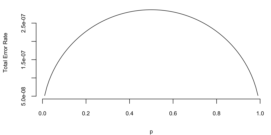
\[ \newcommand{\prob}[1]{\operatorname{P}\left(#1\right)} \newcommand{\Var}[1]{\operatorname{Var}\left(#1\right)} \newcommand{\sd}[1]{\operatorname{sd}\left(#1\right)} \newcommand{\Cor}[1]{\operatorname{Corr}\left(#1\right)} \newcommand{\Cov}[1]{\operatorname{Cov}\left(#1\right)} \newcommand{\E}[1]{\operatorname{E}\left(#1\right)} \newcommand{\defeq}{\overset{\text{\tiny def}}{=}} \DeclareMathOperator*{\argmax}{arg\,max} \DeclareMathOperator*{\argmin}{arg\,min} \DeclareMathOperator*{\mini}{minimize} \]
The hypothesis testing problem is as follows. Based on a sample of data, \(y\), generated from \(p\left( y \mid \theta\right)\) for \(\theta\in\Theta\), the goal is to determine if \(\theta\) lies in \(\Theta_{0}\) or in \(\Theta_{1}\), two disjoint subsets of \(\Theta\). In general, the hypothesis testing problem involves an action: accepting or rejecting a hypothesis. The problem is described in terms of a null, \(H_{0}\), and alternative hypothesis, \(H_{1}\), which are defined as \[ H_{0}:\theta\in\Theta_{0}\;\;\mathrm{and}\;\;H_{1}% :\theta\in\Theta_{1}\text{.}% \]
Different types of regions generate different types of hypothesis tests. If the null hypothesis assumes that \(\Theta_{0}\) is a single point, \(\Theta _{0}=\theta_{0}\), this is known as a simple or “sharp” null hypothesis. If the region consists of multiple points than the hypothesis is called a composite, which occurs if the space is unconstrained or an interval of the real line. In the case of a single parameter, typical one-sided tests are of the form \(H_{0}:\theta<\theta_{0}\) and \(H_{1}:\theta>\theta_{0}\).
There are correct decisions and two types of possible errors. The correct decisions are accepting a null or alternative that is true. A Type I error incorrectly rejects a true null, and a Type II error incorrectly accepts a false null.
| \(\theta\in\Theta_{0}\) | \(\theta\in\Theta_{1}\) | |
|---|---|---|
| Accept \(H_{0}\) | Correct decision | Type II error |
| Accept \(H_{1}\) | Type I error | Correct decision |
Formally, the probabilities of Type I (\(\alpha\)) and Type II (\(\beta\)) errors are defined as: \[ \alpha=P \left[ \text{reject }H_{0} \mid H_{0}\text{ is true }\right] \text{ and }\beta=P \left[ \text{accept }H_{0} \mid H_{1}\text{ is true }\right] \text{.}% \]
It is useful to think of the decision to accept or reject as a decision rule, \(d\left( y\right)\). In many cases, the decision rules form a critical region \(R\), such that \(d\left( y\right) =d_{1}\) if \(y\in R\). These regions are often take the form of simple inequalities. Next, defining the decision to accept the null is \(d\left( y\right) =d_{0}\), and the decision to accept the alternative is \(d_{1},\) the error types are \[\begin{align*} \alpha_{\theta}\left( d\right) & =P \left[ d\left( y\right) =d_{1} \mid \theta\right] \text{ if }\theta\in\Theta_{0}\text{ }(H_{0}\text{ is true})\\ \beta_{\theta}\left( d\right) & =P \left[ d\left( y\right) =d_{0} \mid \theta\right] \text{ if }\theta\in\Theta_{1}\text{ }(H_{1}\text{ is true})\text{.}% \end{align*}\] where both types of errors explicitly depend on the decision and the true parameter value. Notice that both of these quantities are determined by the population properties of the data. In the case of a composite null hypothesis, the size of the test (the probability of making a type I error) is defined as \[ \alpha = \underset{\theta\in\Theta_{0}}{\sup}~\alpha_{\theta}\left( d\right) \] and the power is defined as \(1-\beta_{\theta}\left( d\right)\). It is always possible to set either \(\alpha_{\theta}\left( d\right)\) or \(\beta_{\theta }\left( d\right)\) equal to zero, by finding a test that always rejects alternative or null, respectively.
The total probability of making an error is \(\alpha_{\theta}\left(d\right) +\beta_{\theta}\left(d\right)\), and ideally one would seek to minimize the total error probability, absent additional information. The optimal action \(d^*\) minimizes the posterior expected loss, is \(d^* = d_0 = 0\) if the posterior probability of hypothesis \(H_0\) exceeds 1/2, and \(d^* = d_1=1\) else \[ d^* = 1\left( P \left( \theta \in \Theta_0 \mid y\right) < P \left( \theta \in \Theta_1 \mid y\right)\right) = 1\left(P \left( \theta \in \Theta_0 \mid y\right)<1/2\right). \] Simply speaking, the hypothesis with higher posterior probability is selected.
In thinking of these tradeoffs, it is important to note that the easiest way to reduce the error probability is to gather more data, as the additional evidence should lead to more accurate decisions. In some cases, it is easy to characterize optimal tests, those that minimize the sum of the errors. Simple hypothesis tests of the form \(H_{0}:\theta=\theta_{0}\) versus \(H_{1}:\theta=\theta_{1}\), are one such case admiting optimal tests. Defining \(d^{\ast}\) as a test accepting \(H_{0}\) if \(a_{0}f\left( y \mid \theta_{0}\right) >a_{1}f\left( y \mid \theta_{1}\right)\) and \(H_{1}\) if \(a_{0}f\left( y \mid \theta_{0}\right) <a_{1}f\left( y \mid \theta _{1}\right)\), for some \(a_{0}\) and \(a_{1}\). Either \(H_{0}\) or \(H_{1}\) can be accepted if \(a_{0}f\left(y \mid \theta_{0}\right) =a_{1}f\left( y \mid \theta_{1}\right)\). Then, for any other test \(d\), it is not hard to show that \[ a_{0}\alpha\left( d^{\ast}\right) +a_{1}\beta\left( d^{\ast}\right) \leq a_{0}\alpha\left( d\right) +a_{1}\beta\left( d\right), \] where \(\alpha_{d}=\alpha_{d}\left( \theta\right)\) and \(\beta_{d}=\beta_{d}\left( \theta\right)\). This result highlights the optimality of tests defining rejection regions in terms of the likelihood ratio statistic, \(f\left( y \mid \theta_{0}\right)/f\left( y \mid \theta_{1}\right)\). It turns out that the results are in fact stronger. In terms of decision theoretic properties, tests that define rejection regions based on likelihood ratios are not only admissible decisions, but form a minimal complete class, the strongest property possible.
One of the main problems in hypothesis testing is that there is often a tradeoff between the two goals of reducing type I and type II errors: decreasing \(\alpha\) leads to an increase in \(\beta\), and vice-versa. Because of this, it is common to fix \(\alpha_{\theta}\left( d\right)\), or \(\sup~\alpha_{\theta}\left( d\right)\), and then find a test to minimize \(\beta_{d}\left( \theta\right)\). This leads to “most powerful” tests. In thinking of these tests, there is an important result from decision theory: test procedures that use the same size level of \(\alpha\) in problems with different sample sizes are inadmissible. This is commonly done where significance is indicated by a fixed size, say 5%. The implications of this will be clearer below in examples.
Given observed data \(y\) and likelihood function \(l(\theta) = p(y\mid \theta)\), the likelihood principle states that all relevant experimental information is contained in the likelihood function for the observed \(y\). Furthermore, two likelihood functions contain the same information about \(\theta\) if they are proportional to each other. For example, the widely used maximum-likelihood estimation does satisfy the likelihood principle. However, this principle is sometimes violated by non-Bayesian hypothesis testing procedures. The likelihood principle is a fundamental principle in statistical inference, and it is a key reason why Bayesian procedures are often preferred.
Example 7.1 (Testing fairness) Suppose we are interested in testing \(\theta\), the unknown probability of heads for possibly biased coin. Suppose, \[ H_0 :~\theta=1/2 \quad\text{v.s.} \quad H_1 :~\theta>1/2. \] An experiment is conducted and 9 heads and 3 tails are observed. This information is not sufficient to fully specify the model \(p(y\mid \theta)\). There are two approaches.
Scenario 1: Number of flips, \(n = 12\) is predetermined. Then number of heads \(Y \mid \theta\) is binomial \(B(n, \theta)\), with probability mass function \[ p(y\mid \theta)= {n \choose x} \theta^x(1−\theta)^{n−x} = 220 \cdot \theta^9(1−\theta)^3 \] For a frequentist, the p-value of the test is \[ P(Y \geq 9\mid H_0)=\sum_{y=9}^{12} {12 \choose y} (1/2)^y(1−1/2)^{12−y} = (1+12+66+220)/2^{12} =0.073, \] and if you recall the classical testing, the \(H_0\) is not rejected at level \(\alpha = 0.05\).
Scenario 2: Number of tails (successes) \(\alpha = 3\) is predetermined, i.e, the flipping is continued until 3 tails are observed. Then, \(Y\) - number of heads (failures) until 3 tails appear is Negative Binomial \(NB(3, 1− \theta)\), \[ p(y\mid \theta)= {\alpha+y-1 \choose \alpha-1} \theta^{y}(1−\theta)^{\alpha} = {3+9-1 \choose 3-1} \theta^9(1−\theta)^3 = 55\cdot \theta^9(1−\theta)^3. \] For a frequentist, large values of \(Y\) are critical and the p-value of the test is \[ P(Y \geq 9\mid H_0)=\sum_{y=9}^{\infty} {3+y-1 \choose 2} (1/2)^{x}(1/2)^{3} = 0.0327. \] We used the following identity here \[ \sum_{x=k}^{\infty} {2+x \choose 2}\dfrac{1}{2^x} = \dfrac{8+5k+k^2}{2^k}. \] The hypothesis \(H_0\) is rejected, and this change in decision is not caused by observations.
According to Likelihood Principle, all relevant information is in the likelihood \(l(\theta) \propto \theta^9(1 − \theta)^3\), and Bayesians could not agree more!
Edwards, Lindman, and Savage (1963, 193) note: The likelihood principle emphasized in Bayesian statistics implies, among other things, that the rules governing when data collection stops are irrelevant to data interpretation. It is entirely appropriate to collect data until a point has been proven or disproven, or until the data collector runs out of time, money, or patience.
Formally, the Bayesian approach to hypothesis testing is a special case of the model comparison results to be discussed later. The Bayesian approach just computes the posterior distribution of each hypothesis. By Bayes rule, for \(i=0,1\) \[ P \left( H_{i} \mid y\right) =\frac{p\left( y \mid H_{i}\right) P \left( H_{i}\right) }{p\left( y\right) }\text{,}% \] where \(P \left( H_{i}\right)\) is the prior probability of \(H_{i}\), \[ p\left( y \mid H_{i}\right) =\int_{\theta \in \Theta_i} p\left( y \mid \ \theta\right) p\left( \theta \mid H_{i}\right) d\theta \] is the marginal likelihood under \(H_{i}\), \(p\left( \theta \mid H_{i}\right)\) is the parameter prior under \(H_{i}\), and \[ p\left( y\right) =p\left( y \mid H_{0}\right) P \left( H_{0}\right) +p\left( y \mid H_{1}\right) P \left( H_{1}\right) . \]
If the hypothesis are mutually exclusive, \(P \left( H_{0}\right) =1-P \left( H_{1}\right)\).
The posterior odds of the null to the alternative is \[ \text{Odds}_{0,1}=\frac{P \left( H_{0} \mid y\right) }{P % \left( H_{1} \mid y\right) }=\frac{p\left( y \mid H_{0}\right) }{p\left( y \mid H_{1}\right) }\frac{P \left( H_{0}\right) }{P \left( H_{1}\right) }\text{.}% \]
The odds ratio updates the prior odds, \(P \left( H_{0}\right) /P \left( H_{1}\right)\), using the Bayes Factor, \[ \mathcal{BF}_{0,1}=\dfrac{p\left(y \mid H_{0}\right)}{p\left( y \mid H_{1}\right)}. \] With exhaustive competing hypotheses\(,\) \(P \left( H_{0} \mid y\right)\) simplifies to \[ P \left( H_{0} \mid y\right) =\left( 1+\left( \mathcal{BF}_{0,1}\right) ^{-1}\frac{\left( 1-P \left( H_{0}\right) \right) }{P \left( H_{0}\right) }\right) ^{-1}\text{,}% \] and with equal prior probability, \(p\left( H_{0} \mid y\right) =\left( 1+\left( \mathcal{BF}_{0,1}\right) ^{-1}\right) ^{-1}\). Both Bayes factors and posterior probabilities can be used for comparing hypotheses. Jeffreys (1961) advocated using Bayes factors, and provided a scale for measuring the strength of evidence that was given earlier. Bayes factors merely indicate that the null hypothesis is more likely if \(\mathcal{BF}_{0,1}>1\), \(p\left( y \mid H_{0}\right) >p\left( y \mid H_{1}\right)\). The Bayesian approach merely compares density ordinates of \(p\left( y \mid H_{0}\right)\) and \(p\left( y \mid H_{1}\right)\), which mechanically involves plugging in the observed data into the functional form of the marginal likelihood.
For a point null, \(H_{0}:\theta=\theta_{0}\), the parameter prior is \(p\left( \theta \mid H_{0}\right) =\delta_{\theta_{0}}\left( \theta\right)\) (a Dirac mass at \(\theta_{0}\)), which implies that \[ p\left( y \mid H_{0}\right) =\int p\left( y \mid \theta_{0}\right) p\left( \theta \mid H_{0}\right) d\theta=p\left( y \mid \theta_{0}\right). \] With a general alternative, \(H_{1}:\theta\neq\theta_{0}\), the probability of the null is \[ P \left( \theta=\theta_{0} \mid y\right) =\frac{p\left( y \mid \theta _{0}\right) P \left( H_{0}\right) }{p\left( y \mid \theta _{0}\right) P \left( H_{0}\right) +\left( 1-p\left( H_{0}\right) \right) \int_{\Theta}p\left( y \mid \theta,H_{1}\right) p\left( \theta \mid H_{1}\right) d\theta}, \] where \(p\left( \theta \mid H_{1}\right)\) is the parameter prior under the alternative. This formula will be used below.
Bayes factors and posterior null probabilities measure the relative weight of evidence of the hypotheses. Traditional hypothesis involves an additional decision or action: to accept or reject the null hypothesis. For Bayesian, this typically requires some statement of the utility/loss codifies the benefits/costs of making a correct or incorrect decisision. The simplest situation occurs if one assumes a zero loss of making a correct decision. The loss incurred when accepting the null (alternative) when the alternative is true (false) is \(L\left( d_{0} \mid H_{1}\right)\) and \(L\left( d_{1} \mid H_{0}\right)\), respectively.
The Bayesian will accept or reject based on the posterior expected loss. If the expected loss of accepting the null is less than the alternative, the rational decision maker will accept the null. The posterior loss of accepting the null is \[ \mathbb{E}\left[ \text{Loss}\mid d_{0},y\right] =L\left( d_{0} \mid H_{0}\right) P \left( H_{0} \mid y\right) +L\left( d_{0} \mid H_{1}\right) P \left( H_{1} \mid y\right) =L\left( d_{0} \mid H_{1}\right) P \left( H_{1} \mid y\right) , \] since the loss of making a correct decision, \(L\left( d_{0} \mid H_{0}\right)\), is zero. Similarly, \[ \mathbb{E}\left[ \text{Loss} \mid d_{1},y\right] =L\left( d_{1} \mid H_{0}\right) P \left( H_{0} \mid y\right) +L\left( d_{1} \mid H_{1}\right) P \left( H_{1} \mid y\right) =L\left( d_{1} \mid H_{0}\right) P \left( H_{0} \mid y\right) . \] Thus, the null is accepted if \[ \mathbb{E}\left[ \text{Loss} \mid d_{0},y\right] <\mathbb{E}\left[ \text{Loss} \mid d_{1},y\right] \Longleftrightarrow L\left( d_{0} \mid H_{1}\right) P \left( H_{1} \mid y\right) <L\left( d_{1} \mid H_{0}\right) P \left( H_{0} \mid y\right) , \] which further simplifies to \[ \frac{L\left( d_{0} \mid H_{1}\right) }{L\left( d_{1} \mid H_{0}\right) }<\frac{P \left( H_{0} \mid y\right) }{P \left( H_{1} \mid y\right) }. \] In the case of equal losses, this simplifies to accept the null if \(P \left( H_{1} \mid y\right) <P \left( H_{0} \mid y\right)\). One advantage of Bayes procedures is that the resulting estimators and decisions are always admissible.
Example 7.2 (Enigma machine: Code-breaking) Consider an alphabet of \(26\) letters. Let \(x\) and \(y\) be two codes of length \(T\). We will look to see how many letters match (\(M\)) and don’t match \(N\). In these sequences. Even though the codes are describing different sentences, when letters are the same, if the same code is being used then the sequence will have a match. To compute the bayes factor we need the joint probabilities \[ P( x,y\mid H_0 ) \; \; \mathrm{ and} \; \; P( x,y\mid H_1 ), \] where under \(H_0\) they are different codes, in which case the joint prob is \(( 1 / A )^{2T}\). For \(H_1\) we first need to know the chance of the same letter matching. If \(p_t\) denotes the frequencies of the use of English letters, then we have this match probability \(m = \sum_{i} p_i^2\) which is about \(2/26\). Hence for a particular set of letters \[ P( x_i , y_i \mid H_1 ) = \frac{m}{A} \; \mathrm{ if} \; x_i =y_i \; \; \mathrm{ and} \; \; P( x_i , y_i \mid H_1 ) = \frac{1-m}{A(A-1)} \; \mathrm{ if} \; x_i \neq y_i. \] Hence the log Bayes factor is \[\begin{align*} \ln \frac{P( x,y\mid H_1 )}{P( x,y\mid H_0 )} & = M \ln \frac{ m/A}{1/A^2} +N \ln \frac{ ( 1-m ) / A(A-1) }{ 1/ A^2} \\ & = M \ln mA + N \ln \frac{ ( 1-m )A }{A-1 } \end{align*}\] The first term comes when you get a match and the increase in the Bayes factor is large, \(3.1\) (on a \(log_{10}\))-scale, otherwise you get a no-match and the Bayes factor decreases by \(- 0.18\).
Example, \(N=4\), \(M=47\) out of \(T=51\), then gives evidence of 2.5 to 1 in favor of \(H_1\)
How long a sequence do you need to look at? Calculate the expected log odds. Turing and Good figured you needed sequences of about length \(400\). Can also look at doubles and triples.
Example 7.3 (Signal Transmission) Suppose that the random variable \(X\) is transmitted over a noisy communication channel. Assume that the received signal is given by \[ Y=X+W, \] where \(W\sim N(0,\sigma^2)\) is independent of \(X\). Suppose that \(X=1\) with probability \(p\), and \(X=−1\) with probability \(1−p\). The goal is to decide between \(X=1\) and \(X=−1\) by observing the random variable \(Y\). We will assume symmetric loss and will accept the hypothesis with the higher posterior probability. This is also sometimes called the maximum a posteriori (MAP) test.
We assume that \(H_0: ~ X = 1\), thus \(Y\mid X_0 \sim N(1,\sigma^2)\), and \(Y\mid X_1 \sim N(-1,\sigma^2)\). The Bayes factor is simply the likelihood ratio \[ \dfrac{p(y\mid H_0)}{p(y \mid H_1)} = \exp\left( \frac{2y}{\sigma^2}\right). \] The propr odds are \(p/(1-p)\), thus the posterior odds are \[ \exp\left( \frac{2y}{\sigma^2}\right)\dfrac{p}{1-p}. \] We choose \(H_0\) (true \(X\) is 1), if the posterior odds are greater than 1, i.e., \[ y > \frac{\sigma^2}{2} \log\left( \frac{p}{1-p}\right) = c. \]
Further, we can calculate the error probabilities of our test. \[ p(d_1\mid H_0) = P(Y<c\mid X=1) = \Phi\left( \frac{c-1}{\sigma}\right), \] and \[ p(d_0\mid H_1) = P(Y>c\mid X=-1) = 1- \Phi\left( \frac{c+1}{\sigma}\right). \] Let’s plot the total error rate as a function of \(p\) and assuming \(\sigma=0.2\) \[ P_e = p(d_1\mid H_0) (1-p) + p(d_0\mid H_1) p \]
sigma <- 0.2
p <- seq(0.01,0.99,0.01)
c <- sigma^2/2*log(p/(1-p))
Pe <- pnorm((c-1)/sigma)*(1-p) + (1-pnorm((c+1)/sigma))*p
plot(p,Pe,type="l",xlab="p",ylab="Total Error Rate")
Example 7.4 (Hockey: Hypothesis Testing for Normal Mean) General manager of Washington Capitals (an NHL hockey team) thinks that their star center player Evgeny Kuznetsov is underperformed and is thinking of trading him to a different team. He uses the number of goals per season as a metric of performance. He knows that historically, a top forward scores on average 30 goals per season with a standard deviation of 5, \(\theta \sim N(30,25)\). In the 2022-2023 season Kuznetsov scored 12 goals. For the number of goals \(X\mid \theta\) he uses normal likelihood \(N(\theta, 36)\). Kuznetsov’s performance was not stable over the years, thus high variance in the likelihood. Thus, the posterior is \(N(23,15)\).
sigma2 = 36
sigma02 = 25
mu=30
y=12
k = sigma02 + sigma2
mu1 = sigma2/k*mu + sigma02/k*y
sigma21 = sigma2*sigma02/k
mu1 23sigma21 15The manager thinks, that Kuznetsov simply had a bad year and his true performance is at least 24 goals per season \(H_0: \theta > 24\), \(H_1: \theta<24\). The posterior probability of \(H_0\) hypothesis is
a = 1-pnorm(24,mu1,sqrt(sigma21))
a 0.36It is less than 1/2, only 36%. Thus, we should reject the null hypothesis. The posterior odds in favor of the null hypothesis is
a/(1-a) 0.56If underestimating (and trading) Kuznetsov is two times more costly than overestimating him (fans will be upset and team spirit might be affected), that is \(L(d_1\mid H_0) = 2L(d_0\mid H_1)\), then we should accept the null when posterior odds are greater than 1/2. This is the case here, 0.55 is greater than 1/2. The posterior odds are in favor of the null hypothesis. Thus, the manager should not trade Kuznetsov.
Kuznetsov was traded to Carolina Hurricanes towards the end of the 2023-2024 season.
Notice, when we try to evaluate a new-comer to the league, we use prior probability of \(\theta > 24\)
a = 1-pnorm(24,mu,sqrt(sigma02))
print(a) 0.88a/(1-a) 7.7Thus, the prior odds in favor of \(H_0\) are 7.7.
Example 7.5 (Hypothesis Testing for Normal Mean: Two-Sided Test) In the case of two sided test, we are interested in testing
Where \(n\) is the sample size and \(\sigma^2\) is the variance (known) of the population. Observed samples are \(Y = (y_1, y_2, \ldots, y_n)\) with \[ y_i \sim N(\theta, \sigma^2). \]
The Bayes factor can be calculated analytically \[ BF_{0,1} = \frac{p(Y\mid \theta = m_0, \sigma^2 )} {\int p(Y\mid \theta, \sigma^2) p(\theta \mid m_0, n_0, \sigma^2)\, d \theta} \] \[ \int p(Y\mid \theta, \sigma^2) p(\theta \mid m_0, n_0, \sigma^2)\, d \theta = \frac{\sqrt{n_0}\exp\left\{-\frac{n_0(m_0-\bar y)^2}{2\left(n_0+n\right)\sigma^2}\right\}}{\sqrt{2\pi}\sigma^2\sqrt{\frac{n_0+n}{\sigma^2}}} \] \[ p(Y\mid \theta = m_0, \sigma^2 ) = \frac{\exp\left\{-\frac{(\bar y-m_0)^2}{2 \sigma ^2}\right\}}{\sqrt{2 \pi } \sigma } \] Thus, the Bayes factor is \[ BF_{0,1} = \frac{\sigma\sqrt{\frac{n_0+n}{\sigma^2}}e^{-\frac{(m_0-\bar y)^2}{2\left(n_0+n\right)\sigma^2}}}{\sqrt{n_0}} \]
\[ BF_{0,1} =\left(\frac{n + n_0}{n_0} \right)^{1/2} \exp\left\{-\frac 1 2 \frac{n }{n + n_0} Z^2 \right\} \]
\[ Z = \frac{(\bar{Y} - m_0)}{\sigma/\sqrt{n}} \]
One way to interpret the scaling factor \(n_0\) is ro look at the standard effect size \[ \delta = \frac{\theta - m_0}{\sigma}. \] The prior of the standard effect size is \[ \delta \mid H_1 \sim N(0, 1/n_0). \] This allows us to think about a standardized effect independent of the units of the problem.
Let’s consider now example of Argon discovery.
air =    c(2.31017, 2.30986, 2.31010, 2.31001, 2.31024, 2.31010, 2.31028, 2.31028)
decomp = c(2.30143, 2.29890, 2.29816, 2.30182, 2.29869, 2.29940, 2.29849, 2.29889)
Our null hypothesis is that the mean of the difference equals to zero. We assume that measurements made in the lab have normal errors, this the normal likelihood. We empirically calculate the standard deviation of our likelihood. The Bayes factor is
y = air - decomp
n = length(y)
m0 = 0
sigma = sqrt(var(air) + var(decomp))
n0 = 1
Z = (mean(y) - m0)/(sigma/sqrt(n))
BF = sqrt((n + n0)/n0)*exp(-0.5*n/(n + n0)*Z^2)
BF 1.9e-91We have extremely strong evidence in favor \(H_1: \theta \ne 0\) hypothesis. The posterior probability of the alternative hypothesis is numerically 1!
a = 1/(1+BF)
a 1Example 7.6 (Hypothesis Testing for Proportions) Let’s look at again at the effectiveness of Google’s new search algorithm. We measure effectiveness by the number of users who clicked on one of the search results. As users send the search requests, they will be randomly processed with Algo 1 or Algo 2. We wait until 2500 search requests were processed by each of the algorithms and calculate the following table based on how often people clicked through
| Algo1 | Algo2 | |
|---|---|---|
| success | 1755 | 1818 |
| failure | 745 | 682 |
| total | 2500 | 2500 |
Here we assume binomial likelihood and use conjugate beta prior, for mathematical convenience. We are putting independent beta priors on the click-through rates of the two algorithms, \(p_1\sim Beta(\alpha_1,\beta_1)\) and \(p_2\sim Beta(\alpha_2,\beta_2)\). The posterior for \(p_1\) and and \(p_2\) are independent betas \[ p(p_1, p_1 \mid y) \propto p_1^{\alpha_1 + 1755 - 1} (1-p_1)^{\beta_1 + 745 - 1}\times p_2^{\alpha_2 + 1818 - 1} (1-p_2)^{\beta_2 + 682 - 1}. \]
The easiest way to explore this posterior is via Monte Carlo simulation of the posterior.
set.seed(92) #Kuzy
y1 <- 1755; n1 <- 2500; alpha1 <- 1; beta1 <- 1
y2 <- 1818; n2 <- 2500; alpha2 <- 1; beta2 <- 1
m = 10000
p1 <- rbeta(m, y1 + alpha1, n1 - y1 + beta1)
p2 <- rbeta(m, y2 + alpha2, n2 - y2 + beta2)
rd <- p2 - p1
plot(density(rd), main="Posterior Difference in Click-Through Rates", xlab="p2 - p1", ylab="Density")
q = quantile(rd, c(.05, .95))
print(q)
5% 95%
0.0037 0.0465 abline(v=q,col="red")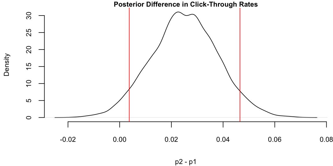
The interval estimators of model parameters are called credible sets. If we use the posterior measure to assess the credibility, the credible set is a set of parameter values that are consistent with the data and gives us is a natural way to measure the uncertainty of the parameter estimate.
Those who are familiar with the concept of classical confidence intervals (CI’s) often make an error by stating that the probability that the CI interval \([L, U ]\) contains parameter is \(1 − \alpha\). The right statement seems convoluted, one needs to generate data from such model many times and for each data set to exhibit the CI. Now, the proportion of CI’s covering the unknown parameter is “tends to” \(1 − \alpha\). Bayesian interpretation of a credible set \(C\) is natural: The probability of a parameter belonging to the set \(C\) is \(1 − \alpha\). A formal definition follows. Assume the set \(C\) is a subset of domain of the parameter \(\Theta\). Then, \(C\) is credible set with credibility \((1 − \alpha)\cdot 100\%\) if \[ p(\theta \in C \mid y) = \int_{C}p(\theta\mid y)d\theta \ge 1 - \alpha. \] If the posterior is discrete, then the integral becomes sum (counting measure) and \[ p(\theta \in C \mid y) = \sum_{\theta_i\in C}p(\theta_i\mid y)d\theta \ge 1 - \alpha. \] This is the definition of a \((1 − \alpha)100\%\) credible set, and of course for a given posterior function such set is not unique.
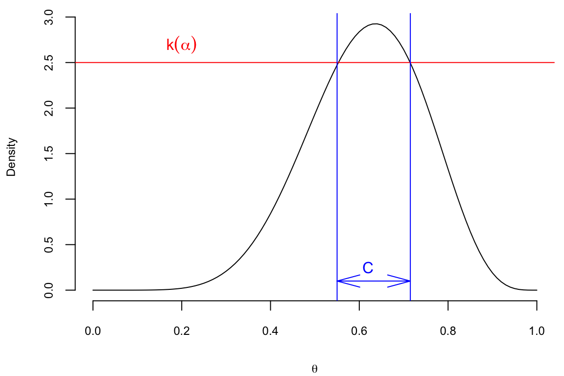
For a given credibility level \((1 − \alpha)100\%\), the shortest credible set is of interest. To minimize size the sets should correspond to highest posterior probability (density) areas. Thus the acronym HPD.
Definition 7.1 (Highest Posterior Density (HPD) Credible Set) The \((1 − \alpha)100\%\) HDP credible set for parameter \(\theta\) is a set \(C \subset \Theta\) of the form \[ C = \{ \theta \in \Theta : p(\theta \mid y) \ge k(\alpha) \}, \] where \(k(\alpha)\) is the smallest value such that \[ P(\theta\in C \mid y) = \int_{C}p(\theta\mid y)d\theta \ge 1 - \alpha. \] Geometrically, if the posterior density is cut by a horizontal line at the hight \(k(\alpha)\), the set \(C\) is projection on the \(\theta\) axis of the part of line inside the density, i.e., the part that lies below the density.
Lemma 7.1 The HPD set \(C\) minimizes the size among all sets \(D \subset \Theta\) for which \[ P(\theta \in D) = 1 − \alpha. \]
Proof. The proof is essentially a special case of Neyman-Pearson lemma. If \(I_C(\theta) = 1(\theta \in C)\) and \(I_D(\theta) = 1(\theta \in D)\), then the key observation is \[ \left(p(\theta\mid y) − k(\alpha)\right)(I_C(\theta) − I_D(\theta)) \ge 0. \] Indeed, for \(\theta\)’s in \(C\cap D\) and \((C\cup D)^c\), the factor \(I_C(\theta)−I_D(\theta) = 0\). If \(\theta \in C\cap D^c\), then \(I_C(\theta)−I_D(\theta) = 1\) and \(p(\theta\mid y)−k(\alpha) \ge 0\). If, on the other hand, \(\theta \in D\cap C^c\), then \(I_C(\theta)−I_D(\theta) = −1\) and \(p(\theta\mid y)−k(\alpha) \le 0\). Thus, \[ \int_{\Theta}(p(\theta\mid y) − k(\alpha))(I_C(\theta) − I_D(\theta))d\theta \ge 0. \] The statement of the theorem now follows from the chain of inequalities, \[ \int_{C}(p(\theta\mid y) − k(\alpha))d\theta \ge \int_{D}(p(\theta\mid y) − k(\alpha))d\theta \] \[ (1-\alpha) - k(\alpha)· size(C) \ge (1-\alpha) - k(\alpha)· size(D) \] \[ size(C) \le size(D). \] The size of a set is simply its total length if the parameter space is one dimensional, total area, if is two dimensional, and so on.
Note, when the distribution \(p(\theta \mid y)\) is unimodal and symmetric using quantiles of the posterior distribution is a good way to obtain the HPD set.
An equal-tailed interval (also called a central interval) of confidence level
\[
I_{\alpha} = [q_{\alpha/2}, q_{1-\alpha/2}],
\] here \(q\)’s are the quantiles of the posterior distribution. This is an interval on whose both right and left side lies \((1-\alpha/2)100\%\) of the probability mass of the posterior distribution; hence the name equal-tailed interval.
Usually, when a credible interval is mentioned without specifying which type of the credible interval it is, an equal-tailed interval is meant.
However, unless the posterior distribution is unimodal and symmetric, there are point outsed of the equal-tailed credible interval having a higher posterior density than some points of the interval. If we want to choose the credible interval so that this not happen, we can do it by using the highest posterior density criterion for choosing it.
Example 7.7 (Cauchy.) Assume that the observed samples
y = c(2,-7,4,-6)come from Cauchy distribution. The likelihood is \[ p(y\mid \theta, \gamma) = \frac{1}{\pi\gamma} \prod_{i=1}^{4} \frac{1}{1+\left(\dfrac{y_i-\theta}{\gamma}\right)^2}. \] We assume unknown location parameter \(\theta\) and scale parameter \(\gamma=1\). For the flat prior \(\pi(\theta) = 1\), the posterior is proportional to the likelihood.
lhood = function(theta) 1/prod(1+(y-theta)^2)
theta <- seq(-10,10,0.1)
post <- sapply(theta,lhood)
post = 10*post/sum(post)
plot(theta,post,type="l",xlab=expression(theta),ylab="Posterior Density")
abline(h=c(0.008475, 0.0159, 0.1, 0.2),col="red")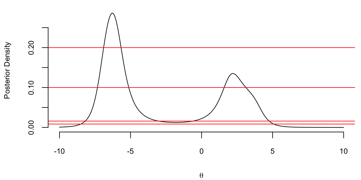
The four horizontal lines correspond to four credible sets
| \(k\) | \(C\) | \(P(\theta \in C \mid y)\) |
|---|---|---|
| 0.008475 | [−8.498, 5.077] | 99% |
| 0.0159 | [−8.189, −3.022] \(\cup\) [−0.615, 4.755] | 95% |
| 0.1 | [−7.328, −5.124] \(\cup\) [1.591, 3.120] | 64.2% |
| 0.2 | [−6.893, −5.667] | 31.2% |
Notice that for \(k = 0.0159\) and \(k = 0.1\) the credible set is not a compact. This shows that two separate intervals “clash” for the ownership of \(\theta\) and this is a useful information. This non-compactness can also point out that the prior is not agreeing with the data. There is no frequentist counterpart for the CI for \(\theta\) in the above model.
The two main alternatives to the Bayesian approach are significance testing using \(p-\)values, developed by Ronald Fisher, and the Neyman-Pearson approach.
Fisher’s approach posits a test statistic, \(T\left( y\right)\), based on the observed data. In Fisher’s mind, if the value of the statistic was highly unlikely to have occured under \(H_{0}\), then the \(H_{0}\) should be rejected. Formally, the \(p-\)value is defined as \[ p=P \left[ T\left( Y\right) >T\left( y\right) \mid H_{0}\right] , \] where \(y\) is the observed sample and \(Y=\left( Y_{1}, \ldots ,Y_{T}\right)\) is a random sample generated from model \(p\left( Y \mid H_{0}\right)\), that is, the null distribution of the test-statistic in repeated samples. Thus, the \(p-\)value is the probability that a data set would generate a more extreme statistic under the null hypothesis, and not the probability of the null, conditional on the data.
The testing procedure is simple. Fisher (1946, p. 80) argues that: *“If P (the p-value) is between* \(0.1\) and \(0.9\), there is is certainly no reason to suspect the hypothesis tested. If it is below \(0.02\), it is strongly indicated that the hypothesis fails to account for the whole of the facts. We shall not be astray if we draw a line at 0.05 and consider that higher values of \(\mathcal{X}^{2}\) indicate a real discrepancy.” Defining \(\alpha\) as the significance level, the tests rejects \(H_{0}\) if \(p<\alpha\). Fisher advocated a fixed significance level of \(5\%\), based largely that \(5\%\) is roughly the tail area of a mean zero normal distribution more than two standard deviations from \(0\), indicating a statistically significant departure. In practice, testing with \(p-\)values involves identifying a critical value, \(t_{\alpha}\), and rejecting the null if the observed statistic \(t\left( y\right)\) is more extreme than \(t_{\alpha}\). For example, for a significance test of the sample mean, \(t\left( y\right) =\left( \overline{y}-\theta_{0}\right) /se\left( \overline{y}\right)\), where \(se\left( \overline{y}\right)\) is the standard error of \(\overline{y}\); the \(5\%\) critical value is 1.96; and Fisher would reject the null if \(t\left( y\right) >t_{\alpha}\).
Fisher interpreted the \(p-value\) as the weight or measure of evidence of the null hypothesis. The alternative hypothesis is noticeable in its absence in Fisher’s approach. Fisher largely rejected the consideration of alternatives, believing that researchers should weigh the evidence or draw conclusions about the observed data rather than making decisions such as accepting or rejecting hypotheses based on it.
There are a number of issues with Fisher’s approach. The first and most obvious criticism is that it is possible to reject the null, when the alternative hypothesis is less likely. This is an inherent problem in using population tail probabilities–essentially rare events. Just because a rare event has occurred does not mean the null is incorrect, unless there is a more likely alternative. This situation often arises in court cases, where a rare event like a murder has occurred. Decisions based on p-values generates a problem called prosecutor’s Fallacy, which is discussed below. Second, Fisher’s approach relies on population properties (the distribution of the statistic under the null) that would only be revealed in repeated samples or asymptotically. Thus, the testing procedure relies on data that is not yet seen, a violation of what is known as the likelihood principle. As noted by Jeffreys’ (1939, pp. 315-316): “What the use of P implies, therefore, is that a hypothesis that may be true may be rejected because it has not predicted observable data that have not occurred. This seems a remarkable procedure”
Third, Fisher is agnostic regarding the source of the test statistics, providing no discussion of how the researcher decides to focus on one test statistic over another. In some simple models, the distribution of properly scaled sufficient statistics provides natural test statistics (e.g., the \(t-\)test). In more complicated models, Fisher is silent on the sources. In many cases, there are numerous test statistics (e.g., testing for normality), and test choice is clearly subjective. For example, in GMM tests, the choice of test moments is clearly a subjective choice. Finally, from a practical perspective, \(p-\)values have a serious deficiency: tests using \(p\)-values often appear to give the wrong answer, in the sense that they provide a highly misleading impression of the weight of evidence in many samples. A number of examples of this will be given below, but in all cases, Fisher’s approach tends to over-reject the null hypotheses.
The motivation for the Neyman-Pearson (NP) approach was W.S. Gosset, the famous `Student’ who invented the \(t-\)test. In analyzing a hypothesis, Student argued that a hypothesis is not rejected unless an alternative is available that provides a more plausible explanation of the data, in which case. Mathematically, this suggests analyzing the likelihood ratio, \[ \mathcal{LR}_{0,1}=\frac{p\left( y \mid H_{0}\right) }{p\left( y \mid H_{1}\right) }\text{,}% \] and rejecting the null in favor of the alternative when the likelihood ratio is small enough, \(\mathcal{LR}_{0,1}<k\). This procedures conforms in spirit with the Bayesian approach.
The main problem was one of finding a value of the cut off parameter \(k.\) From the discussion above, by varying \(k\), one varies the probabilities of type one and type two errors in the testing procedure. Originally, NP argued this tradeoff should be subjectively specified: “how the balance (between the type I and II errors) should be struck must be left to the investigator” (Neyman and Pearson (1933a, p. 296) and “we attempt to adjust the balance between the risks \(P_{1}\)\(P_{2}\) to meet the type of problem before us” (1933b, p. 497). This approach, however, was not “objective *, and they then advocated fixing \(\alpha\), the probability of a type I error, in order to determine \(k\). This led to their famous lemma:
Lemma 7.2 (Neyman-Pearson Lemma) Consider the simple hypothesis test of \(H_{0}:\theta=\theta_{0}\) versus \(H_{1}:\theta =\theta_{1}\) and suppose that the null is rejected if \(\mathcal{LR}_{0,1}<k_{\alpha}\), where \(k_{\alpha}\) is chosen to fix the probability of a type I error at \(\alpha:\)% \[ \alpha=P \left[ y:\mathcal{LR}_{0,1}<k_{\alpha} \mid H_{0}\right] \text{.}% \] Then, this test is the most powerful test of size \(\alpha\) in the sense that any other test with greater power, must have a higher size.
In the case of composite hypothesis tests, parameter estimation is required under the alternative, which can be done via maximum likelihood, leading to the likelihood ratio \[ \mathcal{LR}_{0,1}=\frac{p\left( y \mid H_{0}\right) }{\underset {\theta\in\Theta}{\sup}p\left( y \mid \Theta\right) }=\frac{p\left( y \mid H_{0}\right) }{p\left( y \mid \widehat{\theta}\right) }\text{,}% \] where \(\widehat{\theta}\) is the MLE. Because of this, \(0\leq\mathcal{LR}_{0,1}\leq 1\) for composite hypotheses. In multi-parameter cases, finding the distribution of the likelihood ratio is more difficult, requiring asymptotic approximations to calibrate \(k_{\alpha}.\)
At first glance, the NP approach appears similar to the Bayesian approach, as it takes into account the likelihood ratio. However, like the \(p-\)value, the NP approach has a critical flaw. Neyman and Pearson fix the Type I error, and then minimizes the type II error. In many practical cases, \(\alpha\) is set at \(5\%\) and the resulting \(\beta\) is often very small, close to 0. Why is this a reasonable procedure? Given the previous discussion, this is essentially a very strong prior over the relative benefits/costs of different types of errors. While these assumptions may be warranted in certain settings, it is difficult to a priori understand why this procedure would generically make sense. The next section highlights how the \(p-\)value and NP approaches can generate counterintuitive and even absurd results in standard settings.
This section provides a number of paradoxes arising when using different hypothesis testing procedures. The common strands of the examples will be discussed at the end of the section.
Example 7.8 (Neyman-Pearson tests) Consider testing \(H_{0}:\mu=\mu_{0}\) versus \(H_{1}:\mu=\mu_{1}\), \(y_{t}\sim\mathcal{N}\left( \mu,\sigma^{2}\right)\) and \(\mu_{1}>\mu_{0}\). For this simple test, the likelihood ratio is given by \[ \mathcal{LR}_{0,1}=\frac{\exp\left( -\frac{1}{2\sigma^{2}}% %TCIMACRO{\tsum \nolimits_{t=1}^{T}}% %BeginExpansion {\textstyle\sum\nolimits_{t=1}^{T}} %EndExpansion \left( y_{t}-\mu_{0}\right) ^{2}\right) }{\exp\left( -\frac{1}{2\sigma ^{2}}% %TCIMACRO{\tsum \nolimits_{t=1}^{T}}% %BeginExpansion {\textstyle\sum\nolimits_{t=1}^{T}} %EndExpansion \left( y_{t}-\mu_{1}\right) ^{2}\right) }=\exp\left( -\frac{T}{\sigma^{2}% }\left( \mu_{1}-\mu_{0}\right) \left( \overline{y}-\frac{1}{2}\left( \mu_{0}+\mu_{1}\right) \right) \right) \text{.}% \] Since \(\mathcal{BF}_{0,1}=\mathcal{LR}_{0,1}\), assuming equal prior probabilities and symmetric losses, the Bayesian accepts \(H_{0}\) if \(\mathcal{BF}_{0,1}>1\). Thus, the Bayes procedure rejects \(H_{0}\) if \(\overline{y}>\frac{1}{2}\left( \mu_{0}+\mu_{1}\right)\) for any \(T\) and \(\sigma^{2}\), with \(\mu_{0}\),\(\mu_{1}\), \(T,\)and \(\sigma^{2}\) determining the strength of the rejction. If \(\mathcal{BF}_{0,1}=1\), there is equal evidence for the two hypotheses.
The NP procedure proceeds by first setting \(\alpha=0.05,\) and rejects when \(\mathcal{LR}_{0,1}\) is large. This is equivalent to rejecting when \(\overline{y}\) is large, generating an `optimal’ rejection region of the form \(\overline{y}>c\). The cutoff value \(c\) is calibrated via the size of the test, \[ P \left[ reject\text{ }H_{0} \mid H_{0}\right] =P \left[ \overline{y}>c \mid \mu_{0}\right] =P \left[ \frac{\left( \overline{y}-\mu_{0}\right) }{\sigma/\sqrt{T}}>\frac{\left( c-\mu_{0}\right) }{\sigma/\sqrt{T}} \mid H_{0}\right] . \] The size equals \(\alpha\) if \(\sqrt{T}\left( c-\mu_{0}\right) /\sigma =z_{\alpha}\). Thus, the NP test rejects if then if \(\overline{y}>\mu _{0}+\sigma z_{\alpha}/\sqrt{T}\). Notice that the tests rejects regardless of the value of \(\mu_{1}\), which is rather odd, since \(\mu_{1}\) does not enter into the size of the test only the power. The probability of a type II error is \[ \beta=P \left[ \text{accept }H_{0} \mid H_{1}\right] =P \left[ \overline{y}\leq\mu_{0}+\frac{\sigma}{\sqrt{T}}z_{\alpha } \mid H_{1}\right] =\int_{-\infty}^{\mu_{0}+\frac{\sigma}{\sqrt{T}% }z_{\alpha}}p\left( \overline{y} \mid \mu_{1}\right) d\overline{y}\text{,}% \] where \(p\left( \overline{y} \mid \mu_{1}\right) \sim\mathcal{N}\left( \mu _{1},\sigma^{2}/T\right)\).
These tests can generate strikingly different conclusions. Consider a test of \(H_{0}:\mu=0\) versus \(H_{1}:\mu=5\), based on \(T=100\) observations drawn from \(y_{t}\sim\mathcal{N}\left( \mu,10^{2}\right)\) with \(\overline{y}=2\). For NP, since \(\sigma/\sqrt{T}=1\), \(\overline{y}\) is two standard errors away from \(0\), thus \(H_{0}\) is rejected at the 5% level (the same conclusion holds for \(p-\)values). Since \(p(\overline {y}=2 \mid H_{0})=0.054\) and \(p(\overline{y}=2 \mid H_{1})=0.0044\), the Bayes factor is \(\mathcal{BF}_{0,1}=12.18\) and \(P \left( H_{0} \mid y\right) =92.41\%\). Thus, the Bayesian is quite sure the null is true, while Neyman-Pearson reject the null.
The paradox can be seen in two different ways. First, although \(\overline{y}\) is actually closer to \(\mu_{0}\) than \(\mu_{1}\), the NP test rejects \(H_{0}\). This is counterintuitive and makes little sense. The problem is one of calibration. The classical approach develops a test such that 5% of the time, a correct null would be rejected. The power of the test is easy to compute and implies that \(\beta=0.0012\). Thus, this testing procedure will virtually never accept the null if the alternative is correct. For Bayesian procedure, assuming the prior odds is \(1\) and \(L_{0}=L_{1}\), then \(\alpha=\beta=0.0062\). Notice that the overall probability of making an error is 1.24% in the Bayesian procedure compared to 5.12% in the classical procedure. It should seem clear that the Bayesian approach is more reasonably, absent a specific motivation for inflating \(\alpha\). Second, suppose the null and alternative were reversed, testing \(H_{0}:\mu=\mu_{1}\) versus \(H_{1}:\mu=\mu_{0}\) In the previous example, the Bayes approach gives the same answer, while NP once again rejects the null hypothesis! Again, this result is counterintuitive and nonsensical, but is common when arbitrarily fixing \(\alpha\), which essentially hardwires the test to over-reject the null.
Example 7.9 (Lindley’s paradox) Consider the case of testing whether or not a coin is fair, based on observed coin flips, \[ H_{0}:\theta=\frac{1}{2}\text{ versus }H_{1}:\theta \neq\frac{1}{2}\text{,}% \] based on \(T\) observations from \(y_{t}\sim Ber\left( \theta\right)\). As an example, Table 7.1 provides 4 datasets of differing lengths. Prior to considering the formal hypothesis tests, form your own opinion on the strength of evidence regarding the hypothesis in each data set. It is common for individuals, when confronted with this data to conclude that the fourth sample provides the strongest of evidence for the null and the first sample the weakest.
| #1 | #2 | #3 | #4 | |
|---|---|---|---|---|
| # Flips | 50 | 100 | 400 | 10,000 |
| # Heads | 32 | 60 | 220 | 5098 |
| Percentage of heads | 64 | 60 | 55 | 50.98 |
Fisher’s solution to the problem posits an unbiased estimator, the sample mean, and computes the \(t-\)statistic, which is calculated under \(H_{0}\): \[ t\left( y\right) =\frac{\overline{y}-E\left[ \overline{y} \mid \theta _{0}\right] }{se\left( \overline{y}\right) }=\sqrt{T}\left( 2\widehat {\theta}-1\right) \text{,}% \] where \(se\left(\overline{y}\right)\) is the standard error of \(\overline{y}\). The Bayesian solution requires marginal likelihood under the null and alternative, which are \[ p\left( y \mid \theta_{0}=1/2\right) =\prod_{t=1}^{T}p\left( y_{t} \mid \theta _{0}\right) =\left( \frac{1}{2}\right) ^{\sum_{t=1}^{T}y_{t}}\left( \frac{1}{2}\right) ^{T-\sum_{t=1}^{T}y_{t}}=\left( \frac{1}{2}\right) ^{T}, \tag{7.1}\] and, from Equation 7.1, \(p\left( y \mid H_{1}\right) =B\left( a_{T},A_{T}\right) /B\left(a,A\right)\) assuming a beta prior distribution.
To compare the results, note first that in the datasets given above, \(\widehat{\theta}\) and \(T\) generate \(t_{\alpha}=1.96\) in each case. Thus, for a significance level of \(\alpha=5\%\), the null is rejected for each sample size. Assuming a flat prior distribution, the Bayes factors are \[ \mathcal{BF}_{0,1}=\left\{ \begin{array} [c]{l}% 0.8178\text{ for }N=50\text{ }\\ 1.0952\text{ for }N=100\\ 2.1673\text{ for }N=400\\ 11.689\text{ for }N=10000 \end{array} \right. , \] showing increasingly strong evidence in favor of \(H_{0}\). Assuming equal prior weight for the hypotheses, the posterior probabilities are 0.45, 0.523, 0.684, and 0.921, respectively. For the smallest samples, the Bayes factor implies roughly equal odds of the null and alternative. As the sample size increase, the weight of evidence favors the null, with a 92% probabability for \(N=10K\).
Next, consider testing \(H_{0}:\theta_{0}=0\) vs. \(H_{1}:\theta_{0}\neq0,\) based on \(T\) observations from \(y_{t}\sim \mathcal{N}\left( \theta_{0},\sigma^{2}\right)\), where \(\sigma^{2}\) is known. This is the formal example used by Lindley to generate his paradox. Using \(p-\)values, the hypothesis is rejected if the \(t-\)statistic is greater than \(t_{\alpha}\). To generate the paradox, consider datasets that are exactly \(t_{\alpha}\) standard errors away from \(\overline{y}\), that is, \(\overline {y}^{\ast}=\theta_{0}+\sigma t_{\alpha}/\sqrt{n}\), and a uniform prior over the interval \(\left( \theta_{0}-I/2,\theta_{0}+I/2\right)\). If \(p_{0}\) is the probability of the null, then, \[\begin{align*} P \left( \theta=\theta_{0} \mid \overline{y}^{\ast}\right) & =\frac{\exp\left( -\frac{1}{2}\frac{T\left( \overline{y}^{\ast}-\theta _{0}\right) ^{2}}{\sigma^{2}}\right) p_{0}}{\exp\left( -\frac{1}{2}% \frac{T\left( \overline{y}^{\ast}-\theta_{0}\right) ^{2}}{\sigma^{2}% }\right) p_{0}+\left( 1-p_{0}\right) \int_{\theta_{0}-I/2}^{\theta_{0}% +I/2}\exp\left( -\frac{1}{2}\frac{T\left( \overline{y}^{\ast}-\theta\right) ^{2}}{\sigma^{2}}\right) I^{-1}d\theta}\\ & =\frac{\exp\left( -\frac{1}{2}t_{\alpha}^{2}\right) p_{0}}{\exp\left( -\frac{1}{2}t_{\alpha}^{2}\right) p_{0}+\frac{\left( 1-p_{0}\right) }% {I}\int_{\theta_{0}-I/2}^{\theta_{0}+I/2}\exp\left( -\frac{1}{2}\left( \frac{\left( \overline{y}^{\ast}-\theta\right) }{\sigma/\sqrt{T}}\right) \right) d\theta}\\ & \geq\frac{\exp\left( -\frac{1}{2}t_{\alpha}^{2}\right) p_{0}}{\exp\left( -\frac{1}{2}t_{\alpha}^{2}\right) p_{0}+\frac{\left( 1-p_{0}\right) }% {I}\sqrt{2\pi\sigma^{2}/T}}\rightarrow1\text{ as }T\rightarrow\infty\text{.}% \end{align*}\] In large samples, the posterior probability of the null approaches 1, whereas Fisher always reject the null. It is important to note that this holds for any \(t_{\alpha}\), thus even if the test were performed at the 1% level or lower, the posterior probability would eventually reject the null.
One potential criticism of the previous examples is the choice of the prior distribution. How do we know that, somehow, the prior is not biased against rejecting the null generating the paradoxes? Under this interpretation, the problem is not with the \(p-\)value but rather with the Bayesian procedure. One elegant way of dealing with the criticism is search over priors and prior parameters that minimize the probabability of the null hypothesis, thus biasing the Bayesian procedure against accepting the null hypothesis.
To see this, consider the case of testing \(H_{0}:\mu_{0}=0\) vs. \(H_{1}:\mu_{0}\neq0\) with observations drawn from \(y_{t} \sim\mathcal{N}\left( \theta_{0},\sigma^{2}\right)\), with \(\sigma\) known. With equal prior null and alternative probability, the probability of the null is \(p\left( H_{0} \mid y\right) =\left( 1+\left( \mathcal{BF}_{0,1}\right) ^{-1}\right) ^{-1}\). Under the null, \[ p\left( y \mid H_{0}\right) =\left( \frac{1}{2\pi\sigma^{2}}\right) ^{\frac{T}{2}}\exp\left( -\frac{1}{2}\left( \frac{\left( \overline {y}-\theta_{0}\right) }{\sigma/\sqrt{T}}\right) ^{2}\right) \text{.}% \] The criticism applies to the priors under the alternative. To analyze the sensitivity, consider four classes of priors under the alternative: (a) the class of normal priors, \(p\left( \theta \mid H_{1}\right) \sim\mathcal{N}\left( a,A\right)\); (b) the class of all symmetric unimodal prior distributions; (c) the class of all symmetric prior distributions; and (d) the class of all proper prior distributions. These classes provide varying degrees of prior information, allowing a thorough examination of the strength of evidence.
In the first case, consider the standard conjugate prior distribution, \(p\left( \mu \mid H_{1}\right) \sim\mathcal{N}\left( \mu_{0},A\right)\). Under the alternative, \[\begin{align*} p\left( y \mid H_{1}\right) & =\int p\left( y \mid \mu,H_{1}\right) p\left( \mu \mid H_{1}\right) d\mu\\ & =\int p\left( \overline{y} \mid \mu,H_{1}\right) p\left( \mu \mid H_{1}\right) d\mu\text{,}% \end{align*}\] using the fact that \(\overline{y}\) is a sufficient statistic. Noting that \(p\left( \overline{y} \mid \mu,H_{1}\right) \sim N\left( \mu ,\sigma^{2}/T\right)\) and \(p\left( \mu \mid H_{1}\right) \sim N\left( \mu_{0},A\right)\), we can use the “substitute” instead of integrate trick to assert that \[ \overline{y}=\mu_{0}+\sqrt{A}\eta+\sqrt{\sigma^{2}/T}\varepsilon\text{,}% \] where \(\eta\) and \(\varepsilon\) are standard normal. Then, \(p\left( \overline{y} \mid H_{1}\right) \sim\mathcal{N}\left( \mu_{0},A+\sigma^{2}/T\right)\). Thus, \[ \mathcal{BF}_{0,1}=\frac{p\left( y \mid H_{0}\right) }{p\left( y \mid H_{1}\right) }=\frac{p\left( \overline{y} \mid H_{0}\right) }{p\left( \overline{y} \mid H_{1}\right) }=\frac{\left( \sigma^{2}/T\right) ^{-\frac{1}{2}}}{\left( \sigma^{2}/T+A\right) ^{-\frac{1}{2}}}\frac {\exp\left( -\frac{1}{2}t^{2}\right) }{\exp\left( -\frac{1}{2}\frac {z^{2}\sigma^{2}/T}{A+\sigma^{2}/T}\right) }\text{.} \label{BF_normal}% \] To operationalize the test, \(A\) must be selected. \(A\) is chosen to minimizing the posterior probabilities of the null, with \(P_{norm}\left( H_{0} \mid y\right)\) being the resulting lower bound on the posterior probability of the null. For \(z\geq1\), the lower bound on the posterior probability of the null is \[ P_{norm}\left( H_{0} \mid y\right) =\left[ 1+\sqrt{e}\exp\left( -.5t^{2}\right) \right] ^{-1}, \] which is derived in a reference cited in the notes. This choice provides a maximal bias of the Bayesian approach toward rejecting the null. It is important to note that this is not a reasonable prior, as it was intentionally constructed to bias the null toward rejection.
For the class of all proper prior distributions, it is also easy to derive the bound. From equation above, minimizing the posterior probability is equivalent to minimizing the Bayes factor, \[ \mathcal{BF}_{0,1}=\frac{p\left( y \mid H_{0}\right) }{p\left( y \mid H_{1}\right) }\text{.}% \] Since \[ p\left( y \mid H_{1}\right) =\int p\left( y \mid \theta,H_{1}\right) p\left( \theta \mid H_{1}\right) d\theta\leq p\left( y \mid \widehat{\theta}_{MLE},H_{1}\right) \text{,}% \] where \(\widehat{\theta}_{MLE}=\arg\underset{\theta\neq0}{\max}p\left( y \mid \theta\right)\). The maximum likelihood estimator, maximizes the probability of the alternative, and provides a lower bound on the Bayes factor, \[ \underline{\mathcal{BF}}_{0,1}=\frac{p\left( y \mid H_{0}\right) }{\underset{\theta\neq0}{\sup}p\left( y \mid \theta\right) }\text{.}% \] In this case, the bound is particularly easy to calculate and is given by \[ P_{all}\left( H_{0} \mid y\right) =\left( 1+\exp\left( -\frac{t^{2}}{2}\right) \right) ^{-1}\text{.}% \] A reference cited in the notes provides the bounds for the second and third cases, generating \(P_{s,u}\left( H_{0} \mid y\right)\) and \(P_{s}\left( H_{0} \mid y\right)\), respectively. All of the bounds only depend on the \(t-\)statistic and constants.
Table 7.2 reports the \(t-\)statistics and associated \(p-\)values, with the remaining columns provide the posterior probability bounds. For the normal prior and choosing the prior parameter \(A\) to minimize the probability of the null, the posterior probability of the null is much larger than the \(p-\)value, in every case. For the standard case of a \(t-\)statistic of 1.96, \(P\left( H_{0} \mid y\right)\) is more than six times greater than the \(p-\)value. For \(t=2.576\), \(P\left( H_{0} \mid y\right)\) is almost 13 times greater than the \(p-\)value. These probabilities fall slightly for more general priors. For example, for the class of all priors, a t-statistic of 1.96/2.576 generates a lower bound for the posterior probability of 0.128/0.035\(,\) more than 2/3 times the \(p-\)value.
| \(t\)-stat | \(p\)-value | \(P_{norm}\left(H_{0} \mid y\right)\) | \(P_{s,u}\left( H_{0} \mid y\right)\) | \(P_{s}\left(H_{0} \mid y\right)\) | \(P_{all}\left(H_{0} \mid y\right)\) |
|---|---|---|---|---|---|
| 1.645 | 0.100 | 0.412 | 0.39 | 0.34 | 0.205 |
| 1.960 | 0.050 | 0.321 | 0.29 | 0.227 | 0.128 |
| 2.576 | 0.010 | 0.133 | 0.11 | 0.068 | 0.035 |
| 3.291 | 0.001 | 0.0235 | 0.018 | 0.0088 | 0.0044 |