1 Probability and Uncertainty

“It is remarkable that a science which began with the consideration of games of chance should have become the most important object of human knowledge…”—Pierre-Simon Laplace, 1812

Probability deals with randomness and provides a language to communicate uncertainty, which is usually associated with our lack of knowledge or information. In the classical coin toss, for instance, if we knew the exact force applied, we could predict the outcome with certainty. However, practically it is never the case, and we treat coin toss outcome as random.

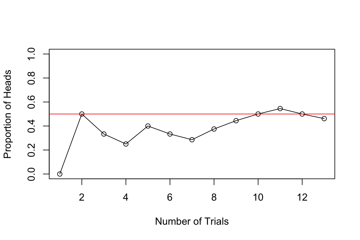
Assigning probabilities to events is a challenging problem. Often, the probability will be applied to analyze the results of experiments (observed data). Consider the coin-tossing example. Say event $A$ represents a Head. Then, to empirically estimate the probability of event $A$, $P(A)$, we can repeat the tossing experiment $N$ times and count $n$, the number of times $A$ occurred. The plot below shows the proportion of heads after $N$ trials.

Graph of the proportion of heads after $N$ trials.

We can see that as $N$ grows, the curve converges to $0.5$. This is the law of large numbers. When $N$ is large, $n/N$ will be close to $P(A)$. The probability as a limit definition is natural and was proposed by von Mises. \[ P(\text{Heads}) = \lim_{N \to \infty} \frac{n}{N}. \]

However, this definition is not operational. It requires the notion of a collective, an infinite sequence of repeatable trials with random outcomes. This is an untestable assumption and was criticized by Ville (1939). On the other hand, Kolmogorov tried to operationalize probability by proposing tests for randomness in his work on algorithmic complexity theory.

We can use a relaxed definition due to Bernoulli and define probability as simply the ratio of the number of heads to the total number of trials in a given experiment. This definition is operational and can be used to estimate the probability of an event. This definition requires the experiment to be repeated under identical conditions. If we are to repeat this experiment under different conditions, e.g., when an unbalanced coin is used, our estimate of $P(A)$ will change as well.

An alternative operational definition of probability was proposed by Frank Ramsey (1926) and later refined by Bruno de Finetti (1937). Rather than relying on long-run frequencies, this approach defines probability through the lens of rational betting behavior. The key insight is that your probability assignment for an event should correspond to the odds at which you would be willing to bet on that event.

de Finetti and Ramsey school of thought takes probability as subjective, namely personal to the observer. De Finetti famously concluded that “Probability does not exist.” Measuring uncertainty is personal to the observer. It’s not like mass which is a property of an object. If two different observers have differing “news,” then there is an opportunity for them to bet (exchange contracts), thus leading to an assessment of probability.

For many events, most people will agree on their probabilities, for example, $P(\text{Heads}) = 0.5$. In the subjective view of probability, we can measure or elicit a personal probability as a “willingness to play”. Namely, will you be willing to bet $1 so you can get $2 if the coin lands Tail and $0 if Head occurs? The subjective view of probability also leads to subjective expected utility theory. You cannot separate the two. For more details, see Chapter 4.

This book primarily adopts the Bayesian (subjective) interpretation of probability, formalized through coherence (the Dutch book principle here, and de Finetti’s representation in Chapter 3). We still use frequentist language and long-run intuition as operational tools, but the organizing viewpoint is probabilistic modeling and belief updating.

Suppose you believe the probability of an event $A$ is $p$. According to Ramsey’s definition, this means you should be indifferent between paying $p \cdot S$ dollars to receive $S$ dollars if event $A$ occurs (and nothing otherwise) and accepting $p \cdot S$ dollars to pay someone $S$ dollars if event $A$ occurs. However, not all probability assignments lead to rational behavior. Suppose someone assigns probabilities to events in an incoherent way. In that case, a clever adversary could construct a series of bets, called a Dutch book, where the individual is guaranteed to lose money regardless of which events occur. The requirement that probabilities must be assigned in such a way that no Dutch book can be constructed against you is known as coherence. For a detailed derivation of probability rules using Dutch Book arguments, see the Appendix.

The principle of coherence for subjective probability is the fundamental rationality constraint, in finance, that would be called the no-arbitrage condition (Poincaré 1952; Bachelier 1900).

Let us consider a simple example. Suppose you assign probability $P(A) = 0.7$ to event $A$ occurring and probability $P(\bar A) = 0.2$ to event $A$ not occurring, where $\bar A$ denotes the complement of $A$. A Dutch book can be constructed as follows:

Bet 1: Pay $\$0.70$ to receive $\$1$ if $A$ occurs
Bet 2: Pay $\$0.20$ to receive $\$1$ if $\bar A$ occurs

Your total payment is $\$0.90$, but you will receive exactly $\$1$ regardless of whether $A$ or $\bar A$ occurs, for a guaranteed loss of $\$0.10$. The incoherence arises because $P(A) + P(\bar A) = 0.9 \neq 1$.

More generally, coherence implies that probabilities must satisfy the following basic properties:

Non-negativity: For any event $A$, we must have $P(A) \geq 0$
Normalization: For the certain event $\Omega$ (the sample space), we must have $P(\Omega) = 1$
Additivity: For mutually exclusive events $A$ and $B$ (i.e., $A \cap B = \emptyset$), we must have $P(A \cup B) = P(A) + P(B)$

To see why non-negativity must hold, suppose $P(A) = -0.1$ for some event $A$. According to the betting interpretation, you would receive $\$0.10$ and then pay $\$1$ if $A$ occurs. If $A$ does not occur, you keep the $\$0.10$ but receive nothing. However, this means you are offering to pay someone to take a bet against $A$, clearly irrational behavior. While standard probability theory requires non-negativity, extensions involving negative probabilities have been explored in fields like physics and quantum computing, as well as in Bayesian modeling as mixing distributions for unobserved latent variables (Polson and Sokolov 2025).

The normalization requirement $P(\Omega) = 1$ ensures that you assign probability one to something that is certain to happen. If $P(\Omega) < 1$, you would be willing to pay less than $\$1$ to receive $\$1$ with certainty, allowing an arbitrageur to make a riskless profit. Conversely, if $P(\Omega) > 1$, you would pay more than $\$1$ for a certain payoff of $\$1$, guaranteeing a loss.

The additivity axiom ensures consistency across mutually exclusive events. If $A$ and $B$ cannot both occur, then betting on “$A$ or $B$” should cost the same as placing separate bets on $A$ and on $B$. Violating this principle again opens the door to Dutch books.

Another axiom $P(A) + P(\bar A) = 1$ just follows from the normalization requirement and the additivity axiom.

These are precisely the axioms proposed by Andrey Kolmogorov (1933) in his foundational work on probability theory. They provide a mathematical structure to probability. Although Kolmogorov’s axioms are agnostic to any definition of probability and are purely mathematical in nature, the fact that they can be derived from the Dutch book argument shows their applicability to rational decision-making under uncertainty. Any violation of these axioms opens you to guaranteed losses through carefully constructed bets. However, Kolmogorov’s axiomatic approach helps us to derive results in more complex settings. For example, Kolmogorov’s framework is applicable in infinite sample spaces and continuous random variables.

The axioms provide a number of rules that probabilities must follow. There are several important corollaries that can help us assign probabilities to events. Here are some important corollaries that follow from the Kolmogorov axioms:

Complement rule: Let “not $A$” denote the complement of event $A$. \[ P(\text{not } A) = 1- P(A). \]
Monotonicity: If $A\subset B$, then $P(A)\le P(B)$. In other words, the probability of a larger set is greater than or equal to the probability of a subset.
Subadditivity: This is a generalization of the addition rule, where the equality holds when events $A$ and $B$ are mutually exclusive. \[ P(A \text{ or } B)\le P(A)+P(B). \]
Inclusion–exclusion principle: This principle extends subadditivity to the case where $A$ and $B$ are not necessarily mutually exclusive. \[ P(A\text{ or } B)=P(A)+P(B)-P(A\text{ and }B). \]
Conditional probability: The conditional probability of $A$ given $B$ is \[ P(A\mid B) = \dfrac{P(A \text{ and } B)}{P(B)}. \]
Bayes’ rule simply reverses the conditioning to compute $P(A\mid B)$ from $P(B\mid A)$, a disciplined probability accounting. \[ P(A\mid B) = \dfrac{P(B\mid A)P(A)}{P(B)}. \]
Law of total probability is a direct consequence of the definition of conditional probability and the normalization axiom. It states that if $B_1, B_2, \ldots, B_n$ are mutually exclusive and exhaustive events, then \[ P(A) = \sum_{i=1}^n P(A \text{ and } B_i) = \sum_{i=1}^n P(A \mid B_i)P(B_i). \]

All of these axioms follow simply from the principle of coherence and the avoidance of Dutch book arbitrage. This includes Bayes’ rule itself (de Finetti 1937; Shimony 1955). If there is arbitrage present in the market, it should be “traded”. It often happens when subjective probabilities do not match.

Bayes’ rule is a fundamental rule of probability that allows us to calculate conditional probabilities. It is a direct consequence of the definition of conditional probability and the normalization axiom. This rule will become central to learning and inference in artificial intelligence.

Bayes’ rule simply provides a disciplined probability accounting of how probabilities get updated in light of evidence. A rational agent requires that their subjective probabilities must obey the principle of coherence. Namely in announcing the set of probabilities, they cannot undergo a sure loss. This is enough to provide a similar framework to the axiomatic approach of Kolmogorov.

These corollaries and principles help in deriving further results and provide additional tools for analyzing and understanding probability and random processes based on the fundamental principles laid out by Kolmogorov. Arguably the most important rule is Bayes’ rule for conditional probability.

The rise of artificial intelligence has renewed the prominence of Bayesian inference in modern learning algorithms. One of the key properties of probabilities is that they are updated as you learn new information. Conditional means given its personal characteristics or the personal situation. Personalization algorithms used by many online services rely on this concept. One can argue that all probabilities are conditional in some way. The process of Bayesian updating is central to how machines learn from observed data. Rational human behavior ought to adhere to Bayes’ rule, although there is much literature documenting the contrary.

1.1 Odds as Probabilities

Another way, sometimes more convenient, to talk about uncertainty and to express probabilities via odds, such as 9 to 2 or 3 to 1. Odds express the ratio of favorable to unfavorable outcomes (Success:Failure), while probability is the chance of an event happening out of all possibilities (Success / Total).

We assign odds “on $A$” (or “in favor of $A$”) versus odds “against $A$”. For example, if the probability of a Chicago Bears’ Super Bowl win is $P(A) = 2/11$, the odds against them are $(1 - 2/11) / (2/11) = 9/2$, or “9 to 2”. This means for every 2 times they win, they lose 9 times. Conventionally, “odds on” often refers to the reverse, but to avoid ambiguity, we will speak of probability or odds against. \[ O(A) = \dfrac{P(\bar A) }{P(A)} = \dfrac{1-P(A)}{P(A)} \] Equivalently, probabilities can be determined from odds \[ P(A) = \dfrac{1}{1+O(A)} \] For example, if the odds are one $O(A) = 1$, then for every $1 bet, you will pay out $1. This event has a probability $0.5$.

If $O(A) = 2$, then you are willing to offer $2:1$. For a $1 bet, you’ll payback $3. In terms of probability, $P(A) = 1/3$.

Odds are primarily used in betting markets. For example, let’s re-analyze the 2016 election in the US.

Example 1.1 (Odds) One of the main sources of prediction markets is bookmakers who take bets on outcomes of events (mostly sporting) at agreed-upon odds. Figure 1.1 shows the odds used by several bookmakers to take bets on the winner of the US presidential election in 2016. At that time, the market was predicting that Hillary Clinton would win over Donald Trump, the second favorite, with odds of 7/3. The table is generated by the Oddschecker website.

Ahead of time, we can assign probabilities of winning to each candidate. According to the bookmakers’ odds, the candidate with the highest chance to win is Hillary Clinton. The best odds on Clinton are $1/3$; this means that you have to risk $3 to win $1 offered by Matchbook. Odds dynamically change as new information arrives. There is also competition between the Bookmakers and the Market is adapting to provide the best possible odds. Ladbrokes is the largest UK bookie, and Betfair is an online exchange. A bookmaker sets their odds trying to get equal public action on both sides, otherwise they are risking to stay out of business.

Example 1.2 (Kentucky Derby) The Kentucky Derby happens once a year—the first Saturday in May. In horse racing, the odds are set by the betting public. The racetrack collects all the bets, takes a fee (18%), and then redistributes the pool to the winning tickets. The race is $1 \frac{1}{4}$ miles (2 kilometers) and is the first time the three-year old horses have raced the distance.

There was a long period where favorites rarely won. Only six favorites have won in the 35 year period from 1979 to 2013. Recently, favorites have won many times in a row. The market is getting better at predicting who’s going to win. Here’s the data

Horse Name	Year	Odds
Spectacular Bid	1979	3/5
Fusaichi Pegasus	2000	2.3/1
Street Sense	2007	9/2
Big Brown	2008	5/2

Recently, favorites have had a lot more success

Horse Name	Year	Odds
California Chrome	2014	5/2
American Pharoah	2015	2/1
Nyquist	2016	3.3/1
Always Dreaming	2017	5.2/1

The most famous favorite to win is Secretariat (1973), who won with odds of 3/2 in a record time of 1 minute 59 and 2/5 seconds. Monarchos was the only other horse that in 2001 had broken two minutes at odds of 11.5/1.

Example 1.3 (Exacta Betting and the Harville Formula) How can probability help you with betting on the race? There are many different types of bets, and probability can help you find fair odds. The Derby is a Grade 1 stakes race for three-year-old thoroughbred horses. Colts and geldings carry 126 pounds, and fillies 121. The odds are set by pari-mutuel betting by the public. After all the wagers have been placed, the racetrack takes a fee (18%). After the winning horse passes the finishing line, the pool of money is redistributed to the winning tickets. Random betting therefore loses you 18%, so it’s important to learn some empirical facts to try and tilt the odds in your favor.

For example, you can place bets as follows:

Win: “$2 win horse 1”
Straight Exacta: “$2 exacta 1 with 2”
Exacta Box: “$2 exacta box 1 and 2” You win with either order: 2 bets = $4.

Consider a hypothetical race where Sovereignty wins at 9/1 odds, and Journalism comes second at 7/2 odds. For a $2 bet on Sovereignty to Win at 9/1, the payout would be $\$2 \cdot 9 + 2 = \$20$ (the 9/1 win plus your initial $2 bet returned).

Let’s figure out the fair value for an exacta bet given that you know the win odds. This is known as the Harville formula. The exacta is a widely used bet among horseplayers, corresponding to predicting the first two horses in the correct order.

The Harville formula provides an answer. We use the rule of conditional probability. The probability for the straight exacta of horse $A$ beating horse $B$ is: \[ P(A \text{ beats } B) = P(A \text{ Wins}) \cdot P(B \text{ Second} \mid A \text{ Wins}) \]

A reasonable assessment of $P(B \text{ Second} \mid A \text{ Wins})$ can be derived as follows. Renormalizing the probabilities by removing the winner $A$ and distributing the probability mass to the remaining horses gives: \[ P(B \text{ Second} \mid A \text{ Wins}) = \frac{P(B \text{ Wins})}{1 - P(A \text{ Wins})} \]

In total, the fair price for the exacta is: \[ P(A \text{ beats } B) = P(A \text{ Wins}) \cdot \frac{P(B \text{ Wins})}{1 - P(A \text{ Wins})} \]

Therefore, we have: \[ p_{12} = p_1 \cdot \frac{p_2}{1-p_1} \text{ where } p_1 = \frac{1}{1+O_1}, p_2 = \frac{1}{1+O_2} \]

Solving for odds, we get the Harville formula: \[ O_{12} = O_1(1 + O_2) - 1 \]

Using our example with 9/1 and 7/2 odds: $O_{12} = 9 \cdot (1 + 3.5) - 1 = 39.5/1$.

Notice that the actual payout is determined solely by the volume of money wagered on that combination. There’s no requirement that it matches our probabilistic analysis. However, the Harville formula gives us an idea of fair value. Some bettors searching for value try to find significantly undervalued exacta bets relative to the Harville formula.

There are many other factors to consider: jockey performance, bloodlines, and post positions can all matter significantly in determining the actual race outcome.

Example 1.4 (Boy-Girl Paradox) If a woman has two children and one is a girl, the chance that the other child is also female has to be $50-50$, right? But it’s not. Let’s list the possibilities of girl-girl, girl-boy and boy-girl. So the chance that both children are girls is 33 percent. Once we are told that one child is female, this extra information constrains the odds. (Even weirder, the author demonstrates that the odds change again if we’re told that one of the girls is named Florida.) In terms of conditional probability, the four possible combinations are \[ BB \; \; BG \; \; GB \; \; GG \] Conditional on the information that one is a girl means that you know we can’t have the $BB$ scenario. Hence, we are left with three possibilities \[ BG \; \; GB \; \; GG \] In one of these is the other, a girl. Hence $1/3$.

It’s a different question if we say that the first child is a girl. Then the probability that the other is a girl is $1/2$, as there are two possibilities \[ GB \; \; GG \] This leads to the probability of $1/2$.

Example 1.5 (Galton Paradox) You flip three fair coins. What is the $P(\text{all} \; \text{alike})$?

Assuming a fair coin (i.e., $P(H) = P(T) = 1/2$), a formal approach might consist of computing the probability for all heads or all tails, which is

\[\begin{align*} P(HHH) &\equiv P(H \text{ and } H \text{ and } H) \\ &= P(H)\times P(H)\times P(H) = \left(\frac{1}{2}\right)^3 \end{align*}\] and, since we’re ultimately interested in the probability of either (mutually exclusive) case, \[\begin{align*} P(\text{all alike}) &= P(HHH \text{ or } TTT) \\ &= P(HHH) + P(TTT) = 2 \times \frac{1}{8} \end{align*}\]

One could arrive at the same conclusion by enumerating the entire sample space and counting the events. Now, what about a simpler argument like the following. In a run of three coin flips, two coins will always share the same result, so the probability that the “remaining/last” coin matches the other two is 1/2; thus, \[ P(\text{all alike}) = 1/2 \] There are 8 equally likely outcomes. Two are ‘all alike’ (HHH, TTT). So 2/8 = 1/4. The error in reasoning is assuming that ‘two must correspond’ fixes the first two coins, but ‘two alike’ could be coins 1&2, 2&3, or 1&3.

For a real treatment of the subject, we highly recommend reading Galton’s essay at galton.org.

Example 1.6 (Three Cards) Suppose that you have three cards: one red/red, one red/blue, and one blue/blue. You randomly draw a card and place it face down on a table, and then you reveal the top side. You see that it’s red. What’s the probability the other side is red? $1/2$? No, it’s $2/3$! By a similar logic, there are six initial possibilities \[ B_1 B_2 \; \; B_2 B_1 \; \; B R \; \; R B \; \; R_1 R_2 \; \; R_2 R_1 \] where $1$ and $2$ index the sides of the same colored cards.

If we now condition on the top side being red, we see that there are still three possibilities left \[ R B \; \; R_1 R_2 \; \; R_2 R_1 \] Hence, the probability is $2/3$ and not the intuitive $1/2$.

Example 1.7 (NFL: New England Patriots Coin Toss) Let’s consider another example and calculate the probability of winning 19 coin tosses out of 25. The NFL team New England Patriots won 19 out of 25 coin tosses in the 2014-15 season. What is the probability of this happening?

Let $X$ be a random variable equal to $1$ if the Patriots win and $0$ otherwise. It’s reasonable to assume $P(X = 1) = \frac{1}{2}$. The probability of observing the sequence in which there is 1 on the first 19 positions, and 0 afterwards is $(1/2)^{25}$. We can code a typical sequence as, \[ 1,1,1,\ldots,1,0,0,\ldots,0. \] There are $177{,}100$ different sequences of 25 games where the Patriots win 19. There are $25! = 1\cdot 2\cdot \ldots \cdot 25$ ways to re-arrange this sequence of zeroes and ones. Further, all zeroes and ones are interchangeable, and there are $19!$ ways to re-arrange the ones and $6!$ ways to rearrange the sequence of zeroes. Thus, the total number of different winning sequences is

factorial(25) / (factorial(19) * factorial(25 - 19))
## 177100

Each potential sequence has a probability $0.5^{25}$, thus \[ P\left(\text{Patriots win 19 out of 25 tosses}\right) = 177{,}100 \times 0.5^{25} = 0.005 \]

Often, it is easier to communicate uncertainties in the form of odds. In terms of betting odds of $1:1$ gives $P = \frac{1}{2}$, odds of $2:1$ (I give $2$ for each $1$ you bet) is $P = \frac{1}{3}$.

Remember, odds, $O(A)$, is the ratio of the probability of happening over not happening, \[ O(A) = (1 - P(A))/P(A), \] equivalently, \[ P(A) = \frac{1}{1 + O(A)}. \]

The odds of the Patriots winning the sequence are then 1 to 199

0.005 / (1 - 0.005)
## 0.005

Example 1.8 (Hitting Streak) Pete Rose of the Cincinnati Reds set a National League record by hitting safely in $44$ consecutive games. How likely is such a long sequence of safe hits to be observed? If you were a bookmaker, what odds would you offer on such an event? This means that he safely reached first base after hitting the ball into fair territory, without the benefit of an error or a fielder’s choice at least once in every one of those 44 games. Here are a couple of facts we know about him:

Rose was a $300$ hitter, he hit safely 3 times out of 10 attempts
Each at bat is assumed to be independent, i.e., the current at bat doesn’t affect the outcome of the next.

Assuming he comes to bat $4$ times each game, what probability might reasonably be associated with that hitting streak? First, we define notation. We use $A_i$ to denote an event of hitting safely at game $i$, then \[ \begin{aligned} & P( \mathrm{Rose \; Hits \; Safely \; in \;44 \; consecutive \; games} ) = \\ & P ( A_1 \; \text{and} \; A_2 \ldots \text{and} \; A_{44} ) = P ( A_1 ) P ( A_2 ) \ldots P ( A_{44} ) \end{aligned} \] We now need to find $P(A_i)$s where $P(A_i) = 1 - P(\text{not} \; A_i)$ \[\begin{align*} P ( A_1 ) & = 1 - P ( \mathrm{ not} \; A_1 ) \\ & = 1 - P ( \mathrm{ Rose \; makes \; 4 \; outs } ) \\ & = 1 - ( 0.7)^4 = 0.76 \end{align*}\] For the winning streak, then we have $(0.76)^{44} = 0.0000057$, a very low probability. In terms of odds, there are three basic inferences

This means that the odds for a particular player as good as Pete Rose, starting a hitting streak today are 175,470 to 1.
This doesn’t mean that the run of $44$ won’t be beaten by some player at some time: the Law of Very Large Numbers
Joe DiMaggio’s record is 56. He is a 325 hitter, thus we have $(0.792)^{56} = 2.13 \times 10^{-6}$ or 469,234 to 1. It’s going to be hard to beat.

The independence assumption underlying this calculation does not account for the popular belief in the “hot hand”, the idea that a player who has been successful recently is more likely to succeed again.

Example 1.9 (Derek Jeter) Sample averages can have paradoxical behavior. This is related to the field of causation and the property of confounding. Let’s compare Derek Jeter’s and David Justice’s batting averages. In both 1995 and 1996, Justice had a higher batting average than Jeter did. However, when you combine the two seasons, Jeter shows a higher batting average than Justice! This is just a property of averages, and finer subset selection can change your average effects.

	1995		1996		Combined
Derek Jeter	12/48	0.250	183/582	0.314	195/630	0.310
David Justice	104/411	0.253	45/140	0.321	149/551	0.270

This situation is known as confounding. It occurs when two separate and different populations are aggregated to give misleading conclusions. The example shows that if $A,B,C$ are events, it is possible to have the three inequalities \[\begin{align*} &P( A \mid B \text{ and } C ) > P( A \mid B \text{ and } \bar C )\\ &P( A \mid \bar B \text{ and } C ) > P( A \mid \bar B \text{ and } \bar C )\\ &P( A \mid C ) < P( A \mid \bar C ) \end{align*}\] The three inequalities can’t hold simultaneously when $P(B\mid C) = P(B\mid \bar C)$.

Example 1.10 (Birthday Problem) The birthday problem (Diaconis and Mosteller 1989) is a classic problem in probability theory that explores the counterintuitive likelihood of shared birthdays within a group. Surprisingly, in a room of 23 people, the probability of shared birthdays is 50%. With 70 people, the probability is 99.9%.

In general, given $N$ items (people) randomly distributed into $c$ categories (birthdays), where the number of items is small compared to the number of categories $N \ll c$, the probability of no match is given by \[ P(\text{no match}) \approx \exp\left(-N^2/2c\right). \] Given $A_i$ is the event that person $i$ has a matching birthday with someone, we have \[ P(\text{no match}) = \prod_{i=1}^{N-1}(1-P(A_i)) = \exp\left(\sum_{i=1}^{N-1}\log (1-P(A_i))\right). \] Here $P(A_i) =\dfrac{i}{c}$ Then use the approximation $\log(1-x) \approx -x$ for small $x$ to get $P(\text{no match})$. \[ \sum_{i=1}^{N-1}\log (1-P(A_i)) \approx -\sum_{i=1}^{N-1}\dfrac{i}{c} = -\dfrac{N(N-1)}{2c}. \]

The probability of at least two people sharing a birthday is then the complement of the probability above: \[ P(\text{At least one shared birthday}) = 1 - P(\text{no match}). \] Solving for $P(\text{match})=1/2$ leads to a square root law $N=1.2\sqrt{c}$, if $c=365$ then $N=23$, and if $c=121$ (near birthday match), then $N=13$.

The unintuitive nature of this result is a consequence of the fact that there are many potential pairs of people in the group, and the probability of at least one pair sharing a birthday increases quickly as more people are added. The birthday problem is often used to illustrate concepts in probability, combinatorics, and statistical reasoning. It’s a great example of how our intuitions about probabilities can be quite different from the actual mathematical probabilities.

1.2 Random Variables: Quantifying Uncertainty

A random variable is a function that maps the outcomes of a random experiment (events) to real numbers. It essentially assigns a numerical value to each outcome in the sample space of a random experiment. In other words, a random variable provides a bridge between the abstract concept of events in a sample space and the concrete calculations involving numerical values and probabilities. Similar to assigning probabilities to events, we can assign respective probabilities to random variables.

For example, consider a random experiment of rolling a die. Here, an event could be “the outcome is an even number”, and the random variable could be the actual number that shows up on the die. The probability of the event “the outcome is an even number” is 0.5, and the probability distribution of the random variable is a list of all numbers from 1 to 6, each with a probability of 1/6.

While events and random variables are distinct concepts, they are closely related through the framework of probability theory, with random variables serving as a key tool for calculating and working with probabilities of events.

Random variables are quantities that we are not certain about. A random variable that can take a finite or a countable number of values is called a discrete random variable (number of rainy days next week). Otherwise, it will be a continuous random variable (amount of rain tomorrow).

Discrete random variables are often constructed by assigning specific values to events such as $\{X=x\}$, which corresponds to the outcomes where $X$ equals a specific number $x$. For example

Will a user click-through on a Google ad? (0 or 1)
Who will win the next presidential election? (Republican=1, Democrat=2, Independent=3)

To fix notation, we will use $P(X=x)$ to denote the probability that random variable $X$ is equal to $x$. A map from all possible values $x$ of a discrete random variable $X$ to probabilities is called a probability mass function $p(x)$. We will interchangeably use $P(X=x)$ and $p(x)$. An important property of the probability mass function is that (normalization Kolmogorov axiom) \[ \sum_{x\in S} p(x) = 1. \] Here $S$ denotes the set of all possible values of random variable $X$.

Clearly, all probabilities have to be greater than or equal to zero, so that $p(x)\ge 0$.

Often, we are interested in \[ F(x) = P(X\le x) = \sum_{y\le x} p(y), \] this is the cumulative distribution function (CDF).

The CDF is a monotonically increasing function (never decreases as $x$ increases). In other words, if $a \leq b$, then $F_X(a) \leq F_X(b)$. The value of the CDF always lies between 0 and 1, inclusive.

Example 1.11 (Discrete CDF) Suppose $X$ is a discrete random variable that represents the outcome of rolling a six-sided die. The probability mass function (PMF) of $X$ is:

\[ P(X = x) = \frac{1}{6} \] for $x = 1, 2, 3, 4, 5, 6$

The CDF of $X$, $F(x)$, is calculated as follows:

For $x < 1$, $F(x) = 0$ (since it’s impossible to roll less than 1).
For $1 \leq x < 2$, $F(x) = \frac{1}{6}$ (the probability of rolling a 1).
For $2 \leq x < 3$, $F(x) = \frac{1}{6} + \frac{1}{6} = \frac{2}{6}$ (the probability of rolling a 1 or 2).
This pattern continues, adding $\frac{1}{6}$ for each integer interval up to 6.
For $x \geq 6$, $F(x) = 1$ (since it’s certain to roll a number 6 or less).

Graphically, the CDF of a discrete random variable is a step function that increases at the value of each possible outcome. It’s flat between these outcomes because a discrete random variable can only take specific, distinct values.

plot(ecdf(1:6), main = "")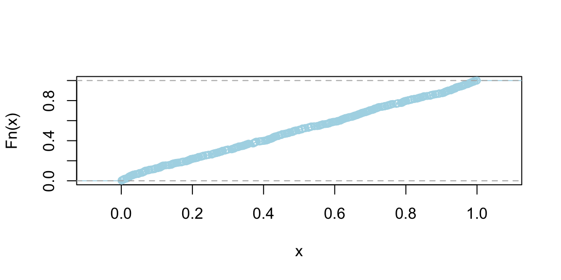

Continuous Random Variables

If we want to build a probabilistic model of a stock price or return, we need to use a continuous random variable that can take an interval of values. Instead of a frequency function we will use a density function, $p(x)$ to describe a continuous variable. Unlike the discrete case, $p(x)$ is not the probability that the random variable takes value $x$. Rather, we need to talk about the value being inside an interval. For example, the probability of $X$ with density $p(x)$ being inside any interval $[a,b]$, with $a<b$ is given by \[ P(a < X < b) = \int_{a}^{b}p(x)dx. \] The total probability is one as $\int_{-\infty}^\infty p(x) dx=1$. The simplest continuous random variable is the uniform. A uniform distribution describes a variable which takes on any value as likely as any other. For example, if you are asked about what would be the temperature in Chicago on July 4 of next year, you might say anywhere between 20 and 30 C. The density function of the corresponding uniform distribution is then \[ p(x) = \begin{cases} 1/10, ~~~20 \le x \le 30\\0, ~~~\mbox{otherwise}\end{cases} \]

Under this model, the probability of temperature being between 25 and 27 degrees is \[ P(25 \le x \le 27) = \int_{25}^{27} p(x)dx = (27-25)/10 = 0.2 \]

Uniform Distribution: Probability of temperature being between 25 and 27.

The Cumulative Distribution Function for a continuous random variable, it is defined similarly to discrete RV CDF as \[ F(x) = P(X \leq x) = \int_{-\infty}^x p(t)dt \] It is a non-decreasing function and takes values in [0,1].

Example 1.12 (Continuous CDF for Uniform Distribution) \[ p(x) = \begin{cases} 1 & \text{if } 0 \leq x \leq 1 \\ 0 & \text{otherwise} \end{cases} \]

The CDF, $F(x)$, is obtained by integrating the PDF:

For $x < 0$, $F(x) = 0$.
For $0 \leq x \leq 1$, $F(x) = \int_0^x 1 \, dt = x$.
For $x > 1$, $F(x) = 1$.

So, the CDF of this uniform distribution is a linear function that increases from 0 to 1 as $x$ goes from 0 to 1.

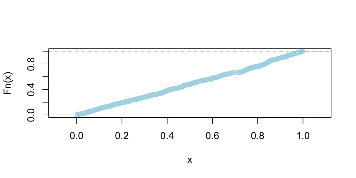
Graphically, the CDF of a continuous random variable is a smooth curve. It starts at 0, increases as $x$ increases, and eventually reaches 1. The exact shape of the curve depends on the distribution of the variable, but the smooth, non-decreasing nature is a common feature. Figure below shows the CDF of a uniform and normal random variable, respectively.

set.seed(33) # Patrick Roy
plot(ecdf(runif(500)), main = "", col = "lightblue", pch = 21, bg = "grey")
plot(ecdf(rnorm(500)), main = "", col = "lightblue", pch = 21, bg = "grey")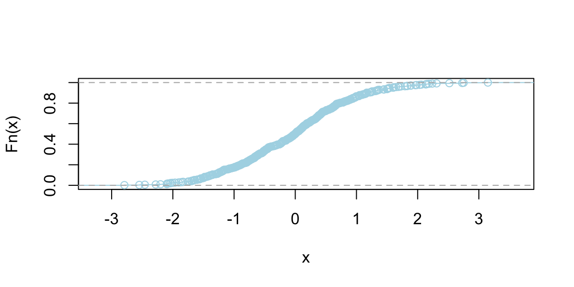

The Inverse CDF Method

The inverse distribution method uses samples of uniform random variables to generate draws from random variables with a continuous distribution function, $F$. Since $F\left( x\right)$ is uniformly distributed on $\left[ 0,1\right]$, draw a uniform random variable and invert the CDF to get a draw from $F$. Thus, to sample from $F$, \[\begin{align*} & \text{Step 1}\text{: Draw }U\sim U\left[ 0,1\right] \ \\ & \text{Step 2}\text{: }\text{Set }X=F^{-1}\left( U\right) , \end{align*}\] where $F^{-1}\left( U\right) =\inf\left\{ x:F\left( x\right) =U\right\}$.

This inversion method provides i.i.d. draws from $F$ provided that $F^{-1}\left( U\right)$ can be exactly calculated. For example, the CDF of an exponential random variable with parameter $\mu$ is $F\left( x\right) =1-\exp\left( -\mu x\right)$, which can easily be inverted. When $F^{-1}$ cannot be analytically calculated, approximate inversions can be used. For example, suppose that the density is a known analytical function. Then, $F\left( x\right)$ can be computed to an arbitrary degree of accuracy on a grid, and inversions can be approximately calculated, generating an approximate draw from $F$. With all approximations, there is a natural trade-off between computational speed and accuracy. One example where efficient approximations are possible are inversions involving normal distributions, which is useful for generating truncated normal random variables. Outside of these limited cases, the inverse transform method does not provide a computationally attractive approach for drawing random variables from a given distribution function. In particular, it does not work well in multiple dimensions.

Functional Transformations

The second main method uses functional transformations to express the distribution of a random variable that is a known function of another random variable. Suppose that $X\sim F$, admitting a density $f$, and that $y=h\left( x\right)$ is an increasing continuous function. Thus, we can define $x=h^{-1}\left( y\right)$ as the inverse of the function $h$. The distribution of $y$ is given by \[ F_Y\left(y\right) =P\left( Y\leq y\right) =\int_{-\infty}^{h^{-1}\left( y\right) }f\left( x\right) dx=F_X\left( X\leq h^{-1}\left(y\right) \right). \] Differentiating with respect to $y$ gives the density via Leibnitz’s rule: \[ f_{Y}\left( y\right) =f\left( h^{-1}\left( y\right) \right) \left\vert\frac{d}{dy}\left( h^{-1}\left( y\right) \right) \right\vert, \] where we make explicit that the density is over the random variable $Y$. This result is used widely. For example, if $X\sim\mathcal{N}\left( 0,1\right)$, then $Y=\mu+\sigma X$. Since $x=h^{-1}\left( y\right) =\frac{y-\mu}{\sigma}$, the distribution function is $F\left( \frac{y-\mu}{\sigma}\right)$ and density \[ f_{Y}\left( y\right) =\frac{1}{\sqrt{2\pi}\sigma}\exp\left( -\frac{1}{2}\left( \frac{y-\mu}{\sigma}\right) ^{2}\right). \] Transformations are widely used to simulate both univariate and multivariate random variables. As examples, if $Y\sim\chi^{2}\left( \nu\right)$ and $\nu$ is an integer, then $Y=\sum_{i=1}^{\nu}X_{i}^{2}$ where each $X_{i}$ is an independent standard normal. Exponential random variables can be used to simulate $\chi^{2}$, Gamma, Beta, and Poisson random variables. The famous Box-Muller algorithm simulates normals from uniform and exponential random variables. In the multivariate setting, Wishart (and inverse Wishart) random variables can be simulated via sums of squared vectors of standard normal random variables.

1.3 Expectation and Variance (Reward and Risk)

An expected value of a random variable, denoted by $\E{X}$ is a weighted average. Each possible value of a random variable is weighted by its probability. For example, Google Maps uses expected value when calculating travel times. We might compute two different routes by their expected travel time. Typically, a forecast or expected value is all that is required; these expected values can be updated in real time as we travel. Say I am interested in the travel time from Washington National Airport to Fairfax, Virginia. The histogram below shows the travel times observed for a work day evening and were obtained from Uber.

Example 1.13 (Uber) Let’s look at the histogram of travel times from Fairfax, VA to Washington, DC

From this dataset, we can empirically estimate the probabilities of observing different values of travel times

Travel Time	Probability
18	0.05
22	0.77
28	0.18

There is a small chance (5%) I can get to Washington, DC in 18 minutes, which probably happens on a holiday, and a non-trivial chance (18%) to travel for 28 minutes, possibly due to a sports game or bad weather. Most of the time (77%), our travel time is 22 minutes. However, when Uber shows you the travel time, it uses the expected value as a forecast rather than the full distribution. Specifically, you will be given an expected travel time of 23 minutes.

0.05 * 18 + 0.77 * 22 + 0.18 * 28
## 23

It is a simple summary that takes into account travel accidents and other events that can affect travel time as best as it can.

The expected value $\E{X}$ of a discrete random variable $X$ which takes possible values $\{x_1,\ldots x_n\}$ is calculated using

\[ \E{X} =\sum_{i=1}^{n}x_i P(X = x_i) \]

For example, in a binary scenario, if $X\in \{0,1\}$ and $P(X=1)=p$, then $\E{X} = 0\times(1-p)+1\times p = p$. The expected value of a Bernoulli random variable is simply the probability of success. In many binary scenarios, a probabilistic forecast is sufficient.

If $X$ is continuous with probability distribution $p(x)$, then we have to calculate the expectation as an integral \[ \E{X} = \int xp(x)d x \text{ and } \int p(x)dx = 1. \]

Standard Deviation and Covariance

Variance measures the spread of a random variable around its expected value $\mu = \E{X}$. For a discrete random variable $X$ with possible values $\{x_1,\ldots x_N\}$, we have \[ \Var{X} = \E{(X-\mu)^2} = \sum_{i=1}^N (x_i-\mu)^2 P(X=x_i). \] In the continuous case, we have \[ \Var{X} = \int_{-\infty}^\infty (x-\mu) ^2 p(x)dx,\text{ where } \mu = \E{X}=\int_{-\infty}^{\infty}x\, p_X(x)dx. \]

The standard deviation is more convenient and is the square root of variance $\sd{X} = \sqrt{\Var{X}}$. Standard deviation has the desirable property that it is measured in the same units as the random variable $X$ itself and is a more useful measure.

Suppose that we have two random variables $X$ and $Y$. We need to measure whether they move together or in opposite directions. The covariance is defined by \[ \Cov{X,Y} = \E{\left[ (X- \E{X})(Y- \E{Y})\right]}. \]

When $X$ and $Y$ are discrete, and we are given the joint probability distribution, we need to calculate \[ \Cov{X,Y} = \sum_{x,y} ( x - \E{X} )(y - \E{Y})p(x,y). \] Covariance is measured in units of $X\times$units of $Y$. This can be inconvenient and makes it hard to compare covariances of different pairs of variables. A more convenient metric is the correlation, which is defined by \[ \Cor{X,Y}= \frac{ \Cov{X,Y} }{ \sd{X} \sd{Y} }. \] Correlation, $\Cor{X,Y}$, is unitless and takes values between -1 and 1.

In the case of joint continuous distribution, it is convenient to use the covariance matrix $\Sigma$ which is defined as \[ \Sigma = \begin{bmatrix} \Var{X} & \Cov{X,Y} \\ \Cov{X,Y} & \Var{Y} \end{bmatrix}. \] If $X$ and $Y$ are independent, then $\Cov{X,Y} = 0$ and $\Sigma$ is diagonal. The correlation matrix is defined as \[ \rho = \begin{bmatrix} 1 & \Cor{X,Y} \\ \Cor{X,Y} & 1 \end{bmatrix}. \] If $X$ and $Y$ have an exact linear relationship, then $\Cor{X,Y} = 1$ and $\Cov{X,Y}$ is the product of standard deviations. In matrix notation, the relation between the covariance matrix and correlation matrix is given by \[ \rho = \mathrm{diag}\left(\Sigma\right)^{-1/2} \Sigma\mathrm{diag}\left(\Sigma\right)^{-1/2}, \] where $\mathrm{diag}\left(\Sigma\right)$ is the diagonal matrix formed from the diagonal (variance) entries of $\Sigma$, so that $\mathrm{diag}\left(\Sigma\right)^{-1/2}$ carries the reciprocal standard deviations on its diagonal.

Portfolios: Linear Combinations

Calculating means and standard deviations of combinations of random variables is a central tool in probability. It is known as the portfolio problem. Let $P$ be your portfolio, which comprises a mix of two assets $X$ and $Y$, typically stocks and bonds, \[ P = aX + bY, \] where $a$ and $b$ are the portfolio weights, typically $a+b=1$, as we are allocating our total capital. Imagine that you have placed $a$ dollars on the random outcome $X$, and $b$ dollars on $Y$. The portfolio $P$ measures your total weighted outcome.

Key portfolio rules: The expected value and variance follow the relations \[\begin{align*} \E{aX + bY} = & a\E{X}+b\E{Y}\\ \Var{ aX + bY } = & a^2 \Var{X} + b^2 \Var{Y} + 2 ab \Cov{X,Y }, \end{align*}\] with covariance defined by \[ \Cov{X,Y} = \E{ ( X- \E{X} )(Y- \E{Y})}. \] Expectation and variance help us to understand the long-run behavior. When we make long-term decisions, we need to use the expectations to avoid biases.

The covariance is related to the correlation by $\Cov{X,Y} = \Cor{X,Y} \sqrt{\Var{X}\,\Var{Y}}$.

Example 1.14 (Tortoise and Hare) Tortoise and Hare are selling cars. Say $X$ is the number of cars sold, and probability distributions, means, and variances are given by the following table

	$X$				Mean	Variance	sd
	0	1	2	3	$\E{X}$	$\Var{X}$	$\sqrt{\Var{X}}$
Tortoise	0	0.5	0.5	0	1.5	0.25	0.5
Hare	0.5	0	0	0.5	1.5	2.25	1.5

Let’s calculate Tortoise’s expectations and variances \[\begin{align*} \E{T} & = (1/2) (1) + (1/2)(2) = 1.5 \\ \Var{T} & = \E{T^2} - \E{T}^2 \\ & = (1/2)(1)^2 + (1/2)(2)^2 - (1.5)^2 = 0.25 \end{align*}\]

Now the Hare’s \[\begin{align*} \E{H} & = (1/2)(0) + (1/2)(3) = 1.5 \\ \Var{H} & = (1/2)(0)^2 + (1/2)(3)^2- (1.5)^2 = 2.25 \end{align*}\]

What do these tell us about the long-run behavior?

Tortoise and Hare have the same expected number of cars sold.
Tortoise is more predictable than Hare. He has a smaller variance.

The standard deviations $\sqrt{\Var{X}}$ are $0.5$ and $1.5$, respectively. Given two equal means, you always want to pick the lower variance. If we are to invest in one of those, we prefer Tortoise.

What about a portfolio of Tortoise and Hare? Suppose I want to evenly split my investment between Tortoise and Hare. What is the expected number of cars sold and the variance of the number of cars sold? \[ \E{\frac{1}{2}T + \frac{1}{2}H} = \frac{1}{2} \E{T} + \frac{1}{2} \E{H} = 1.5 \] For variance, we need to know $\Cov{T,H}$. The standard deviations $0.5$ and $1.5$ cap the covariance at $|\Cov{T,H}| \le 0.5 \times 1.5 = 0.75$, so let’s take the most negative value possible, $\Cov{T,H} = -0.75$ (perfect negative correlation), and see what happens. \[ \begin{aligned} \Var{\frac{1}{2}T + \frac{1}{2}H} &= \frac{1}{4} \Var{T} + \frac{1}{4} \Var{H} + \frac{1}{2} \Cov{T,H} \\ &= 0.0625 + 0.5625 - 0.375 = 0.25 \end{aligned} \]

Notice that the portfolio variance (0.25) equals Tortoise’s own variance and is far below Hare’s (2.25), even though the two assets share the same expected return. This demonstrates the power of diversification: by combining investments with negative covariance, we can reduce overall risk while maintaining the same expected return. The negative covariance indicates that when Tortoise performs well, Hare tends to perform poorly, and vice versa, creating a natural hedge. Tilting the weights toward the steadier asset would lower the variance further still.

This example illustrates a fundamental principle in finance and decision theory: diversification can reduce risk without sacrificing expected returns when assets are not perfectly positively correlated. The key insight is that variance depends not only on individual asset volatilities but also on their covariances, making portfolio construction a crucial consideration in risk management.

1.4 Limiting Behavior of Averages

The Tortoise and Hare example illustrates how expectations and variances behave for a single period or a fixed portfolio. However, in many real-world applications, from insurance to machine learning, we are interested in what happens when we repeat an experiment many times. Does the average outcome settle down to a predictable value?

When we observe a stochastic process repeatedly, we naturally ask: what happens to averages as we collect more data? This question lies at the heart of statistical inference and forms the theoretical foundation for learning from experience. The answer is provided by the law of large numbers, a central result in probability theory.

The Weak Law of Large Numbers

The weak law of large numbers, in its simplest form, states that sample averages converge in probability to the expected value. We assume that observation $x_1, x_2, \ldots, x_n$ are draws (realizations) of independent identically distributed (i.i.d.) random variables $X_1, X_2, \ldots, X_n$ with finite mean $\mu = \E{X_i}$. Then the sample average $\bar{X}_n = \frac{1}{n}\sum_{i=1}^n X_i$ satisfies: \[ \lim_{n \to \infty} P\left(\left|\bar{X}_n - \mu\right| > \epsilon\right) = 0, \] for any $\epsilon > 0$. This form of convergence, known as convergence in probability, means that for large enough $n$, the probability that the sample average deviates from the true mean by more than any fixed amount becomes arbitrarily small.

The proof of this result, when the variance $\sigma^2 = \Var{X_i}$ exists and is finite, follows elegantly from Chebyshev’s inequality. Since $\E{\bar{X}_n} = \mu$ and $\Var{\bar{X}_n} = \sigma^2/n$, we have:

\[ P\left(\left|\bar{X}_n - \mu\right| > \epsilon\right) \leq \frac{\Var{\bar{X}_n}}{\epsilon^2} = \frac{\sigma^2}{n\epsilon^2} \to 0 \]

as $n \to \infty$. This simple argument reveals why averages become more reliable as sample sizes grow: the variance of the sample mean shrinks at a rate $1/n$.

This $1/n$ scaling reappears throughout the book, from confidence intervals and A/B testing (Chapter 5) to the role of sample size in estimation risk and generalization.

Kolmogorov’s Strong Law of Large Numbers

While the weak law establishes convergence in probability, a stronger form of convergence is possible. The strong law of large numbers states that sample averages converge almost surely (with probability one) to the expected value. This is a fundamentally stronger statement: it means that for almost every realization of the sequence, the sample average actually approaches the true mean, not merely that the probability of large deviations vanishes.

Andrey Kolmogorov formalized this result in his 1933 monograph Foundations of the Theory of Probability (Kolmogorov 1933), establishing the conditions under which strong convergence holds. His result placed probability on a rigorous measure-theoretic foundation.

Kolmogorov’s Strong Law states that if $X_1, X_2, \ldots$ are independent random variables (not necessarily identically distributed) with finite variances satisfying Kolmogorov’s condition $\sum_{i=1}^{\infty} \Var{X_i}/i^2 < \infty$, then:

\[ \bar{X}_n = \frac{1}{n}\sum_{i=1}^n X_i \to \mu \quad \text{almost surely} \]

where $\mu = \lim_{n \to \infty} \frac{1}{n}\sum_{i=1}^n \E{X_i}$, provided this limit exists. For i.i.d. random variables the variance condition is not needed: a finite mean $\E{|X_1|} < \infty$ alone gives $\bar{X}_n \to \mu$ almost surely, with $\mu = \E{X_1}$.

The distinction between convergence in probability and almost sure convergence is subtle but crucial. Convergence in probability allows for infinitely many large deviations, as long as they become increasingly rare. Almost sure convergence is stronger: it requires that eventually, after some finite (but random) time, all deviations remain small forever.

Formally, almost sure convergence means:

\[ P\left(\lim_{n \to \infty} \bar{X}_n = \mu\right) = 1 \]

This is equivalent to saying that the set of sequences for which the limit fails to equal $\mu$ has probability zero. For practical purposes, this means we can be confident that the specific sequence we observe will exhibit convergence, not merely that convergence is likely.

The independence assumption is central to Kolmogorov’s results, but it can be relaxed in various ways for different applications. For stochastic processes with dependent observations, the key question becomes: how much dependence can we tolerate while still obtaining convergence of averages?

For stationary processes, where the joint distribution of $(X_t, X_{t+1}, \ldots, X_{t+k})$ does not depend on $t$, a law of large numbers holds under considerably weaker conditions than independence. If the process is ergodic (roughly, if it eventually “forgets” its initial conditions), then time averages converge to ensemble averages:

\[ \frac{1}{n}\sum_{i=1}^n X_i \to \mu \quad \text{almost surely} \]

This ergodic theorem extends Kolmogorov’s law of large numbers to dependent sequences and is central to statistical inference from time series data. It justifies the common practice of estimating population means from a single long realization of a stochastic process.

The law of large numbers is not merely a theoretical curiosity; it forms the bedrock of statistical practice. Every time we estimate a population mean from a sample, test a hypothesis, or train a machine learning model, we implicitly rely on the law of large numbers. The confidence we place in larger samples, the use of cross-validation to assess model performance, and the convergence of stochastic gradient descent in deep learning all trace back to this fundamental result.

In the context of stochastic processes, the law of large numbers justifies estimating process parameters from a single long trajectory. When modeling financial returns, climate data, or network traffic, we typically observe one realization over time rather than multiple independent realizations. The ergodic theorem ensures that time averages from this single path converge to the true population moments, enabling inference from the data we actually have.

The Kolmogorov’s formalization is the culmination of several decades of work on the foundations of probability theory. The weak law of large numbers was first proved by Jakob Bernoulli in 1713 for the special case of binomial random variables, an achievement that took him over twenty years. The result was later generalized by Poisson (1837) and Chebyshev (1867) to broader classes of random variables.

The strong law required deeper mathematical machinery. Émile Borel proved a version for Bernoulli trials in 1909, but the general result awaited the development of measure-theoretic probability. Francesco Cantelli made progress in the 1910s, but it was Kolmogorov who provided the definitive treatment in 1933, unifying diverse results under a single rigorous framework.

Kolmogorov’s work transformed probability theory from a collection of special cases and heuristics into a branch of mathematics with the same rigor as analysis or algebra. His measure-theoretic foundations enabled precise statements about almost sure convergence, clarified the distinction between different modes of convergence, and opened the door to modern probability theory and stochastic processes.

The law of large numbers underpins Bayesian inference and computational statistics. For applications to posterior consistency, Monte Carlo simulation, and Markov chain Monte Carlo (MCMC) methods, see Section 3.11 in Chapter 3.

1.5 Binomial, Poisson, and Normal Distributions

We now examine three fundamental probability distributions that appear throughout statistics and machine learning.

Bernoulli Distribution

The formal model of a coin toss was described by Bernoulli. He modeled the notion of probability for a coin toss, now known as the Bernoulli distribution, where $X \in \{0,1\}$ and $P(X=1)=p, P(X=0) = 1-p$. Laplace gave us the principle of insufficient reason: where you would list out the possibilities and then place equal probability on each of the outcomes. Essentially, the discrete uniform distribution on the set of possible outcomes.

A Bernoulli trial relates to an experiment with the following conditions

The result of each trial is either a success or a failure.
The probability $p$ of a success is the same for all trials.
The trials are assumed to be independent.

The Bernoulli random variable can take on one of two possible outcomes, typically labeled as “success” and “failure.” It is named after the Swiss mathematician Jacob Bernoulli, who introduced it in the 18th century. The distribution is often denoted by $\text{Bernoulli}(p)$, where $p$ is the probability of success.

The probability mass function (PMF) of a Bernoulli distribution is defined as follows: \[ P(X = x) = \begin{cases} p & \text{if } x = 1 \\ 1 - p & \text{if } x = 0 \end{cases} \] The expected value (mean) of a Bernoulli distributed random variable $X$ is given by: \[\E{X} = p \] Simply speaking, if you are to toss a coin many times, you expect $p$ heads.

The variance of $X$ is given by: \[ \Var{X} = p(1-p) \]

Example 1.15 (Coin Toss) The quintessential random variable is an outcome of a coin toss. The set of all possible outcomes, known as the sample space, is $S = \{H,T\}$, and $P(X = H) = P(X = T) = 1/2$. On the other hand, a single outcome can be an element of many different events. For example, there are four possible outcomes of two coin tosses, HH, TT, HT, and TH, which are equally likely with probabilities of 1/4. The probability mass function over the number of heads $X$ out of two coin tosses is

$x$	0	1	2
$p(x)$	1/4	1/2	1/4

Given the probability mass function, we can, for example, calculate the probability of at least one head as $P(X \geq 1) = P(X =1) + P(X =2) = p(1)+p(2) = 3/4$.

The Bernoulli distribution serves as the foundation for more complex distributions, such as the binomial distribution (which models the number of successes in a fixed number of independent Bernoulli trials) and the geometric distribution (which models the number of trials needed to achieve the first success). A Binomial distribution arises from a sequence of Bernoulli trials, and assigns probability to $X$, which is the number of successes. Its probability distribution is calculated via: \[ P(X=x) = {n \choose x} p^x(1-p)^{n-x}. \] Here ${n \choose x}$ is the combinatorial function, \[ {n \choose x} = \frac{n!}{x!(n-x)!}, \] Here the combinatorial function ${n \choose x}$ counts the number of ways of getting $x$ successes in $n$ trials and $n!=n(n-1)(n-2)\ldots 2 \cdot 1$ counts the number of permutations of $n$ observations without replacement.

Plot below shows the probability mass function of a Binomial distribution with $n = 20$ and $p = 0.3$.

barplot(dbinom(0:20, size = 20, prob = 0.3),
  names.arg = 0:20, col = "lightblue",
  xlab = "Number of Heads", ylab = "Probability"
)

Probability Mass Function of a Binomial Distribution (n = 20, p = 0.3).

The table below shows the expected value and variance of a Binomial random variable. Those quantities can be calculated by plugging in the possible outcomes and corresponding probabilities into the definitions of expected value and variance.

Mean and Variance of Binomial.
Binomial Distribution	Parameters
Expected value	$\mu = \E{X} = n p$
Variance	$\sigma^2 = \Var{X} = n p ( 1 - p )$

For large sample sizes $n$, this distribution is approximately normal with mean $np$ and variance of $np(1-p)$.

Let $X$ be the number of heads in three flips. Each possible outcome (“realization”) of $X$ is an event. Now, consider the event of getting only two heads \[ \{ X= 2\} = \{ HHT, HTH, THH \} , \] The probability distribution of $X$ is Binomial with parameters $n = 3, p= 1/2$, where $n$ denotes the sample size (a.k.a. number of trials) and $p$ is the probability of heads; we have a fair coin. The notation is $X \sim \mathrm{Bin} \left ( n = 3 , p = \frac{1}{2} \right )$ where the sign $\sim$ is read as distributed as.

Outcomes of three coin flips.
Result	$X$	$P(X=x)$
HHH	3	$p^3$
HHT	2	$p^2 ( 1- p)$
HTH	2	$p^2 ( 1 - p)$
THH	2	$(1-p)p^2$
HTT	1	$p( 1-p)^2$
THT	1	$p ( 1-p)^2$
TTH	1	$(1-p)^2 p$
TTT	0	$(1-p)^3$

Poisson Distribution

The Poisson distribution is a discrete probability distribution that expresses the probability of a given number of events occurring in a fixed interval of time or space if these events occur with a known constant mean rate and independently of the time since the last event. You can think of Poisson distribution as a limiting case of the Binomial distribution when the number of trials $n$ is large and the probability of success $p$ is small, such that $np = \lambda$ remains constant. Think of a soccer game where the goal is the “successful” event of interest. The soccer team does not have a predefined number of attempts to score a goal. Rather, they continuously try to score a goal until they do. The number of goals scored in a game is the number of events occurring in a fixed interval of time. The mean number of goals scored in a game is the mean rate of events occurring in a fixed interval of time.

There are many examples of Poisson distributed random variables. For example, the number of phone calls received by a call center per hour, the number of emails received per day, the number of customers arriving at a store per hour, the number of defects in a manufactured product, the number of accidents on a highway per month.

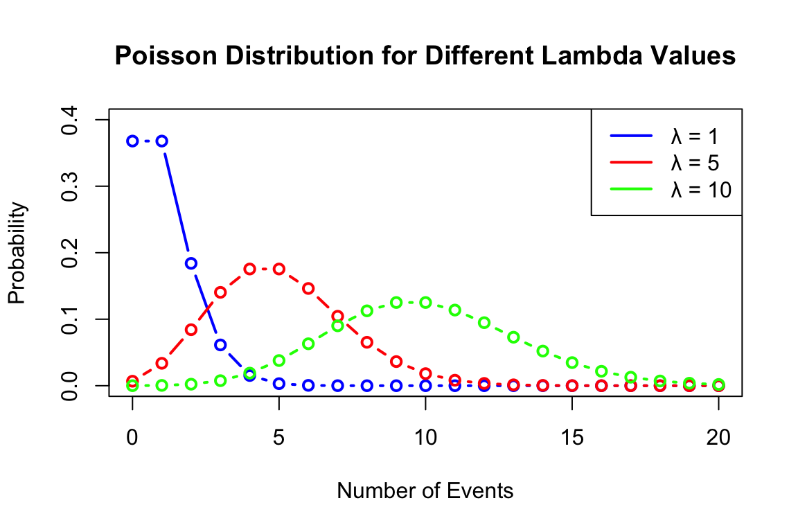
A random variable $X$ follows a Poisson distribution with parameter $\lambda > 0$ if its probability mass function is given by: \[ P(X = k) = \frac{\lambda^k e^{-\lambda}}{k!} \] for $k = 0, 1, 2, 3, \ldots$, where $\lambda$ is both the mean and variance of the distribution.

Plot below shows the probability mass function of a Poisson distribution with $\lambda = 1, 5, 10$.

We write $X \sim \text{Poisson}(\lambda)$ to denote that $X$ follows a Poisson distribution with parameter $\lambda$.

Mean and Variance of Poisson.
Poisson Distribution	Parameters
Expected value	$\mu = \E{X} = \lambda$
Variance	$\sigma^2 = \Var{X} = \lambda$

Example 1.16 (Customer Arrivals) Suppose customers arrive at a coffee shop at an average rate of 3 customers per hour. What is the probability that exactly 5 customers will arrive in the next hour?

Using the Poisson distribution with $\lambda = 3$: \[ P(X = 5) = \frac{3^5 e^{-3}}{5!} = \frac{243 \times e^{-3}}{120} \approx 0.101 \]

So there is approximately a 10.1% chance that exactly 5 customers will arrive in the next hour.

The Poisson distribution can be derived as a limiting case of the binomial distribution when $n$ is large and $p$ is small, such that $np = \lambda$ remains constant. This connection makes the Poisson distribution particularly useful for modeling rare events in large populations.

Normal Distribution

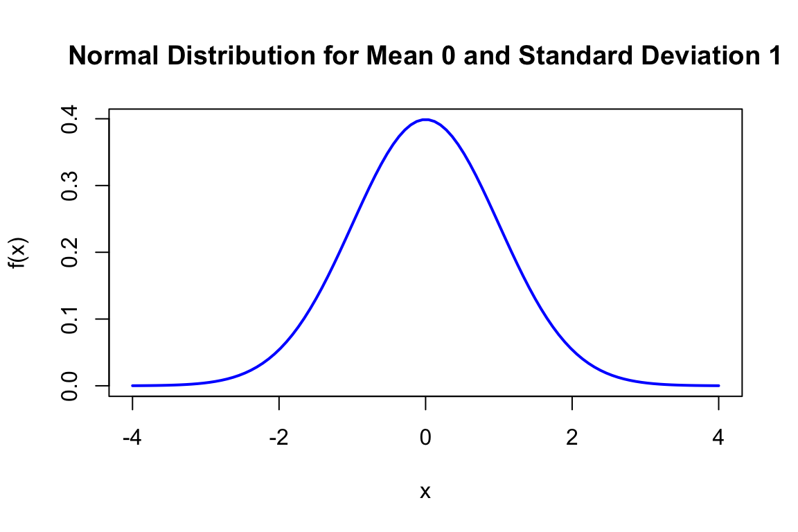
The Normal distribution is a continuous probability distribution that is widely used in statistics and probability theory. It is also known as the Gaussian distribution or the bell curve. The Normal distribution is characterized by its symmetric bell-shaped curve and is defined by two parameters: the mean ($\mu$) and the variance ($\sigma^2$).

The probability density function (PDF) of the Normal distribution is given by: \[ f(x) = \frac{1}{\sigma \sqrt{2\pi}} e^{-\frac{(x-\mu)^2}{2\sigma^2}} \] for $-\infty < x < \infty$, where $\mu$ is the mean and $\sigma$ is the standard deviation.

The Normal distribution is often used to model real-world phenomena such as measurement errors, heights, weights, and scores on standardized tests. It is also used in hypothesis testing and confidence interval construction.

Example 1.17 (Heights of Adults) The heights of adult males in a certain population are normally distributed with a mean of 70 inches and a standard deviation of 3 inches.

What is the probability that a randomly selected male is between 67 and 73 inches tall?

Using the Normal distribution with $\mu = 70$ and $\sigma = 3$:

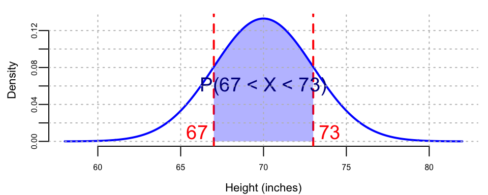
Figure 1.2: Normal Distribution (mu = 70, sigma = 3) with Highlighted Area.

The bell curve in Figure 1.2 shows the probability density function of a random variable $X \sim N(70,3^2)$, a Normal distribution with mean 70 and standard deviation 3. As we can see, the Normal distribution is symmetric around the mean, and the mean, median, and mode are all equal. The probability of a randomly selected male being between 67 and 73 inches tall is the area under the curve between 67 and 73 inches and is approximately 0.6827.

Now let’s calculate this probability using R:

prob_between <- pnorm(73, mean = 70, sd = 3) - pnorm(67, mean = 70, sd = 3)
cat("P(67 < X < 73) =", round(prob_between, 4), "\n")
## P(67 < X < 73) = 0.68

The calculation shows that $P(67 < X < 73) = P(X \leq 73) - P(X \leq 67) \approx 0.6827$.

This result makes sense because 67 and 73 inches are exactly one standard deviation below and above the mean (70 $\pm$ 3), respectively. According to the empirical rule (68-95-99.7 rule), approximately 68% of values in a normal distribution fall within one standard deviation of the mean.

So approximately 68.27% of adult males are between 67 and 73 inches tall.

What height corresponds to the 95th percentile?

We need to find $x$ such that $P(X \leq x) = 0.95$. From standard normal tables, $\Phi^{-1}(0.95) \approx 1.645$.

x <- qnorm(0.95, mean = 70, sd = 3)
cat("Height corresponding to the 95th percentile:", round(x, 2), "inches\n")
## Height corresponding to the 95th percentile: 75 inches

Therefore: $x = \mu + \sigma \cdot 1.645 = 70 + 3 \cdot 1.645 = 74.935$ inches.

Example 1.18 (The 1987 Stock Market Crash) How extreme was the October 1987 crash of $-21.76\%$? We can use standardization to quantify just how unusual this event was under a Normal model.

Prior to the October 1987 crash, S&P 500 monthly returns averaged $1.2\%$ with a volatility (standard deviation) of $4.3\%$. If we model returns as $X \sim N(0.012, 0.043^2)$, we can standardize to obtain a Z-score: \[ Z = \frac{X - \mu}{\sigma} = \frac{X - 0.012}{0.043} \sim N(0,1) \]

For the observed crash return of $-21.76\%$: \[ Z = \frac{-0.2176 - 0.012}{0.043} = -5.34 \]

This is a 5-sigma event. Under the Normal distribution, the probability of observing a return this extreme or more extreme is vanishingly small:

z_score <- (-0.2176 - 0.012) / 0.043
pnorm(z_score)
## 0.000000047

The probability is approximately $4.6 \times 10^{-8}$, or about 1 in 22 million. If returns were truly Normal and independent, we would expect such an event to occur roughly once every 22 million months, or once every 1.8 million years.

This analysis raises an important point about model validation. The Normal distribution, while convenient, may not accurately capture the behavior of financial returns, particularly in the tails. Empirically, stock returns exhibit fat tails, meaning extreme events occur more frequently than the Normal distribution predicts. The 1987 crash, the 2008 financial crisis, and other market disruptions suggest that using an inaccurate model can lead to severely underestimating the probability of extreme events.

1.6 Conditional, Marginal and Joint Distributions

Suppose that we have two random variables $X$ and $Y$, which can be related to each other. Knowing $X$ would change your belief about $Y$. For example, as a first pass, psychologists who study the phenomenon of happiness can be interested in understanding its relation to income level. Now we need a single probability mass function (a.k.a. probabilistic model) that describes all possible values of those two variables. Joint distributions do exactly that.

Formally, the joint distribution of two variables $X$ and $Y$ is a function given by \[ P(x,y) = P(X=x,Y=y). \] This maps all combinations of possible values of these two variables to a probability on the interval [0,1].

The conditional probability is a measure of the probability of a random variable $X$, given that the value of another random variable was observed as $Y = y$. \[ P(x\mid y) = P(X = x \mid Y = y). \]

The marginal probability of a subset of a collection of random variables is the probability distribution of the variables contained in the subset without reference to the values of the other variables. Say we have two random variables $X$ and $Y$, the marginal probability $P(X)$ is the probability distribution of $X$ when the values of $Y$ are not taken into consideration. This can be calculated by summing the joint probability distribution over all values of $Y$. The converse is also true: the marginal distribution can be obtained for $Y$ by summing over the separate values of $X$.

Marginal probability is different from conditional probability. Marginal probability is the probability of a single event occurring, independent of other events. A conditional probability, on the other hand, is the probability that an event occurs given that another specific event has already occurred.

Example 1.19 (Salary-Happiness) Let’s look at an example. Suppose that we want to model the relationship between two quantities, salary $Y$ and happiness $X$. After running a survey, we summarize our results using the joint distribution, which is described by the following “happiness index” table as a function of salary.

Results of the Gallup survey. Rows are Salary ($Y$), and columns are happiness ($X$)
	X = 0 (low)	X = 1 (medium)	X = 2 (high)
Y = low (0)	0.03	0.13	0.14
Y = medium (1)	0.12	0.11	0.01
Y = high (2)	0.07	0.01	0.09
Y = very high (3)	0.02	0.13	0.14

Each cell of the table is the joint probability, e.g., 14% of people have a very high income level and are very happy. Those joint probabilities are calculated by simple counting and calculating the proportions.

Now, if we want to answer the question, what is the percent of high earners in the population. For that, we need to calculate what is called a marginal probability $P(y = 2)$. We can calculate the proportion of high earners $P(y = 2)$ by summing up the entries in the third row of the table, which is 0.17 in our case.

0.07 + 0.01 + 0.09
## 0.17

Formally, marginal probability over $y$ is calculated by summing the joint probability over the other variable, $x$, \[ p(y) = \sum_{x \in S}p(x,y) \] Where $S$ is the set of all possible values of the random variable $X$.

Another question of interest is whether happiness depends on income level. To answer those types of questions, we need to introduce an important concept, which is the conditional probability of $X$ given that the value of variable $Y$ is known. This is denoted by $P(X=x\mid Y=y)$ or simply $p(x\mid y)$, where $\mid$ reads as “given” or “conditional upon”.

The conditional probability $p(x\mid y)$ also has an interpretation as updating your probability over $X$ after you have learned the new information about $Y$. In this sense, probability is also the language of how you change opinions in light of new evidence. The proportion of happy people among high earners is given by the conditional probability $P(X=2\mid Y=2)$ and can be calculated by dividing the proportion of those who are high earners and highly happy by the proportion of high earners \[ P(X=2\mid Y=2) = \dfrac{P(X=2,Y=2)}{P(Y=2)} = \dfrac{0.09}{0.17} = 0.5294118. \]

Now, if we compare it with the proportion of highly happy people, $P(X = 2) = 0.38$, we see that, on average you are more likely to be happy given your income is high.

1.7 Independence

Historically, the concept of independence in experiments and random variables has been a defining mathematical characteristic that has uniquely shaped the theory of probability. This concept has been instrumental in distinguishing the theory of probability from other mathematical theories.

Using the notion of conditional probability, we can define the independence of two variables. Two random variables $X$ and $Y$ are said to be independent if \[ P(Y = y \mid X = x) = P(Y = y), \] for all possible $x$ and $y$ values. That is, learning information $X=x$ doesn’t affect our probabilistic assessment of $Y$ for any value $y$. In the case of independence, $p(x \mid y) = p(x)$ and $p(y \mid x) = p(y)$.

Conditional probabilities are counter-intuitive. For example, one of the most important properties is typically $p( x \mid y ) \neq p( y\mid x )$. Confusing these two, specifically equating $P(A \mid B)$ with $P(B \mid A)$, is a common error known as the Prosecutor’s Fallacy.

We just derived an important relation that allows us to calculate the conditional probability $p(x \mid y)$ when we know joint probability $p(x,y)$ and marginal probability $p(y)$. The total probability or evidence can be calculated as usual, via $p(y) = \sum_{x}p(x,y)$.

We will see that independence will lead to a different conclusion than the Bayes conditional probability decomposition: specifically, independence yields $p( x,y ) = p(x) p(y)$, whereas Bayes implies $p(x ,y) = p(x)p(y \mid x)$.

1.8 Further Notes: Dutch Book Arguments

If probabilities are degrees of belief and subjective, where do they come from and what rules must they satisfy? These questions were answered to varying degrees by Ramsey, de Finetti, and Savage. Ramsey and de Finetti, working independently and at roughly the same time, developed the first primitive theories of subjective probability and expected utility, and Savage placed the theories on a more rigorous footing, combining the insights of Ramsey with the expected utility theory of von Neumann and Morgenstern.

The starting point for Ramsey’s and de Finetti’s theories is the measurement of one’s subjective probabilities using betting odds, which have been used for centuries to gauge the uncertainty over an event. As noted by de Finetti, “It is a question of simply making mathematically precise the trivial and obvious idea that the degree of probability attributed by an individual to a given event is revealed by the conditions under which he would be disposed to bet on that event” (p. 101). Notice the difference between the frequentist and Bayesian approach. Instead of defining the probabilities via an infinite repeated experiment, the Bayesian approach elicits probabilities from an individual’s observed behavior.

Formally, for any event $A$, the identity \[ P(A) =\frac{1}{1+\text{odds}(A)}\text{ or }\text{odds}(A)=\frac{1-P(A)}{P(A)}, \] where $\bar A$ is the complement of $A$, links odds and probabilities. Throughout, we use $P$ as a generic term to denote probabilities when there is no specific reference to an underlying distribution or density. If a horse in a race has odds of 2, commonly expressed as 2:1 (read two to one), then the probability the horse wins is $1/3$. The basic idea of using betting odds to elicit probabilities is simple and intuitive: ask an individual to place odds on various mutually exclusive events, and use these odds to calculate the probabilities. Odds are fair if lower odds would induce a person to take the bet, and higher odds would induce the person to take the other side of the bet.

In constructing a collection of betting odds over various events, de Finetti and Ramsey argued that not all odds are rational (i.e., consistent or coherent). For example, the sum of the probability of each horse winning a race cannot be greater than one. If a person has inconsistent beliefs, then he “could have a book made against him by a cunning bettor and would then stand to lose in any event” (Ramsey (1931), p. 22). This situation is called a Dutch book arbitrage, and a rational theory of probability should rule out such inconsistencies. By avoiding Dutch books, Ramsey and de Finetti showed that the degrees of beliefs elicited from coherent odds satisfy the standard axioms of probability theory, such as the restriction that probabilities are between zero and one, finite additivity, and the laws of conditional probability. The converse also holds: probabilities satisfying the standard axioms generate odds excluding Dutch-book arbitrages. Absence of arbitrage is natural in finance and economics and is a primary assumption for many foundational results in asset pricing. In fact, the derivations given below have a similar flavor to those used to prove the existence of a state price density assuming discrete states.

Dutch-book arguments are simple to explain. To start, they require an individual to post odds on events. A bettor or bookie can then post stakes or make bets at those odds with a given payoff, $S$. The choice of the stakes is up to the bettor. A Dutch book occurs when a cunning bettor makes money for sure by placing carefully chosen stakes at the given odds. Alternatively, one can view the odds as prices of lottery tickets that pay off $1 when the event occurs, and the stakes as the number of tickets bought. Thus, probabilities are essentially lottery ticket prices. In fact, de Finetti used the notation ‘Pr’ to refer to both prices and probabilities.

To derive the rules, consider the first axiom of probability: for any event $A$, $0\leq P(A) \leq 1$. Suppose that the odds imply probabilities $P(A)$ for $A$ occurring and $P(\bar A)$ for other outcomes, with associated payoffs of $S_{A}$ and $S_{\bar A}$. Then, having bet $S_{A}$ and $S_{\bar A}$, the gains if $A$ or $\bar A$ occur, $G_{A}$ and $G_{\bar A}$, respectively, are \[\begin{align*} G(A) & =S_{A}-P(A) S_{A}-P(\bar A) S_{\bar A}\\ G(\bar A) & =S_{\bar A}-P(A) S_{A}-P(\bar A) S_{\bar A}. \end{align*}\] To see this, note that the bettor receives $S_{A}$ and pays $P(A) S_{A}$ for a bet on event $A$. The bookie can always choose to place a zero stake on $\bar A$ occurring, which implies that $G(A) =S_{A}-P(A) S_{A}$ and $G\left(\bar A\right) =-P(A) S_{A}$. Coherence or the absence of arbitrage implies that you cannot gain or lose in both states, thus $G(A) G(\bar A) \leq 0$. Substituting, $\left( 1-P(A) \right) P(A) \geq0$ or $0\leq P(A) \leq 1$, which is the first axiom of probability. The second axiom, that the set of all possible outcomes has probability $1$, is similarly straightforward to show.

The third axiom is that probabilities add, that is, for two disjoint events $A_{1}$ and $A_{2}$, $P(A) =P\left( A_{1} \text{ or } A_{2}\right) =P\left( A_{1}\right) +P\left( A_{2}\right)$. Assuming stakes sizes of $S_{A}$, $S_{A_{1}},$ and $S_{A_{2}}$ (and zero stakes on their complements) there are three possible outcomes. If neither $A_{1}$ nor $A_{2}$ occurs, the gain is \[ G(\bar A) =-P(A) S_{A} -P\left( A_{1}\right) S_{A_{1}}-P\left( A_{2}\right) S_{A_{2}}. \]

If $A_{1}$ occurs, $A$ also occurs, and the gain is \[ G\left( A_{1}\right) =\left( 1-P(A) \right) S_{A}+\left( 1-P\left( A_{1}\right) \right) S_{A_{1}}-P\left( A_{2}\right) S_{A_{2}}, \] and finally, if $A_{2}$ occurs, $A$ also occurs, and \[ G\left( A_{2}\right) =\left( 1-P(A) \right) S_{A}-P\left( A_{1}\right) S_{A_{1}}+\left( 1-P\left( A_{2}\right) \right) S_{A_{2}}. \] Arranging these into a matrix equation, $G=PS$: \[ \left( \begin{array} [c]{c}% G(\bar A) \\ G\left( A_{1}\right) \\ G\left( A_{2}\right) \end{array} \right) =\left( \begin{array} [c]{ccc}% -P(A) & -P\left( A_{1}\right) & -P\left( A_{2}\right) \\ 1-P(A) & 1-P\left( A_{1}\right) & -P\left( A_{2}\right) \\ 1-P(A) & -P\left( A_{1}\right) & 1-P\left( A_{2}\right) \end{array} \right) \left( \begin{array} [c]{c}% S_{A}\\ S_{A_{1}}\\ S_{A_{2}}% \end{array} \right). \]

The absence of a Dutch book arbitrage implies that there is no set of stakes, $S_{A}$, $S_{A_{1}}$, and $S_{A_{2}}$, such that the winnings in all three events are positive. If the matrix $P$ is invertible, it is possible to find stakes with positive gains. To rule this out, the determinant of $P$ must be zero, which implies that $0=-P(A) +P\left(A_{1}\right) +P\left( A_{2}\right)$, or $P\left(A\right) =P\left( A_{1}\right) +P\left( A_{2}\right)$.

The fourth axiom is conditional probability. Consider an event $B$, with $P\left( B\right) >0$, an event $A$ that occurs conditional on $B$, and the event that both $A$ and $B$ occur. The probabilities or prices of these bets are $P\left( B\right)$, $P\left( A \mid B\right)$, and $P\left( A \text{ and } B\right)$. Consider bets with stakes $S_{B}$, $S_{A \mid B}$ and $S_{A \text{ and } B}$, with the understanding that if $B$ does not occur, the conditional bet on $A$ is canceled. The payoffs to the events that $B$ does not occur, $B$ occurs but not $A$, and $A$ and $B$ occur, are \[ \left( \begin{array} [c]{c}% G\left( \bar B\right) \\ G\left( \bar A \text{ and } B\right) \\ G\left( A \text{ and } B\right) \end{array} \right) =\left( \begin{array} [c]{ccc}% -P\left( B\right) & -P\left( A \text{ and } B\right) & 0\\ 1-P\left( B\right) & -P\left( A \text{ and } B\right) & -P\left( A \mid B\right) \\ 1-P\left( B\right) & 1-P\left( A \text{ and } B\right) & 1-P\left( A \mid B\right) \end{array} \right) \left( \begin{array} [c]{c}% S_{B}\\ S_{A \text{ and } B}\\ S_{A \mid B}% \end{array} \right). \] Similar arguments imply that the determinant must be zero, which implies that \[ P\left( A \mid B\right) =\frac{P\left( A \text{ and } B\right) }{P\left( B\right) }, \] which is the law of conditional probability, given $P(B)>0$, of course, otherwise the conditional probability is not defined, and the $P$ matrix has determinant 0.

Exercises

Pen-and-Pencil

Exercise 1.1 (Dutch Book and Coherence) A racetrack analyst states her personal probabilities for an upcoming three-horse race between Alpha, Beta, and Gamma, where exactly one horse wins (no ties, no scratches). She is a coherent forecaster in the betting sense of this chapter: for any of the three outcomes, she will, at her stated price, both buy and sell a contract paying $1 if that horse wins and $0 otherwise, in any quantity you request. Her quotes are \[ P(\text{Alpha wins}) = 0.50, \qquad P(\text{Beta wins}) = 0.35, \qquad P(\text{Gamma wins}) = 0.25. \]

The events {Alpha wins, Beta wins, Gamma wins} are mutually exclusive and exhaustive. Which axiom of probability do these quoted prices violate, and why must that axiom hold for any coherent assignment of probabilities to a partition of the sample space?
You decide to exploit the mispricing. Should you buy or sell contracts on all three horses, and why? Using a common stake $S = \pm 100$ (state the sign), find your net cash flow in each of the three possible worlds (Alpha wins, Beta wins, Gamma wins) and confirm that your profit is identical and strictly positive, no matter which horse wins. This is the explicit Dutch book.
Generalize part (b). A bettor takes an equal, signed stake $S$ on each of $k$ mutually exclusive, exhaustive events with quoted prices $P(A_1), \ldots, P(A_k)$: paying $P(A_i) S$ now for contract $i$, and receiving $S$ back on whichever event occurs. Show that the guaranteed gain is \[ G = S\left(1 - \sum_{i=1}^k P(A_i)\right), \] the same value in every possible world. Use this formula to explain (i) why $\sum_i P(A_i) > 1$ is exploitable by selling ($S<0$), (ii) why $\sum_i P(A_i) < 1$ is exploitable by buying ($S>0$), and (iii) why no Dutch book of this kind exists when $\sum_i P(A_i) = 1$.
The analyst revises her quote to $P(\text{Gamma wins}) = 0.15$, leaving the other two prices unchanged. Is the book now coherent? Use your formula from part (c) to explain why the equal-stake construction can no longer turn a riskless profit.

Exercise 1.2 (Joint Distributions) A credit card company collects data on $10{,}000$ users. The data contained two variables: an indicator of the customer status: whether they are in default (def = 1) or if they are current with their payments (def = 0). Moreover, they have a measure of their loan balance relative to income with three categories: a low balance (bal=1), medium (bal=2), and high (bal=3). The data are given in the following table:

	def
bal	0	1
1	8,940	64
2	651	136
3	76	133

Compute the marginal distribution of customer status
What is the conditional distribution of bal given def = 1
Make a prediction for the status of a customer with a high balance

Exercise 1.3 (Marginal) The table below is taken from the Hoff text and shows the joint distribution of occupations taken from a 1983 study of social mobility by Logan (1983). Each cell is P(father’s occupation, son’s occupation).

	farm	operatives	craftsman	sales	professional
farm	0.02	0.04	0.03	0.01	0.02
operative	0.00	0.11	0.06	0.03	0.07
craftsman	0.00	0.07	0.09	0.03	0.08
sales	0.00	0.02	0.02	0.01	0.05
professional	0.00	0.03	0.03	0.04	0.13

Find the marginal distribution of fathers’ occupations.
Find the marginal distribution of sons’ occupations.
Find the conditional distribution of the son’s occupation given that the father is a farmer.
Find the conditional distribution of the father’s occupation given that the son is a farmer.
Comment on these results. What do they say about changes in farming in the population from which these data are drawn?

Exercise 1.4 (Conditional) Netflix surveyed the general population as to the number of hours per week that you used their service. The following table provides the proportions of each category according to whether you are a teenager or adults.

Hours	Teenager	Adult
$<4$	0.18	0.20
$4$ to $6$	0.12	0.32
$>6$	0.04	0.14

Calculate the following probabilities:

Given that you spend $4$ to $6$ hours a week watching movies, what’s the probability that you are a teenager?
What is the marginal distribution of hours spent watching movies.
Are hours spent watching Netflix movies independent of age?

Exercise 1.5 (Joint and Conditional) The following probability table relates $Y$, the number of TV shows watched by the typical student in an evening, to the number of drinks $X$ consumed.

	Y
X	0	1	2	3
0	0.07	0.09	0.06	0.01
1	0.07	0.06	0.07	0.01
2	0.06	0.07	0.14	0.03
3	0.02	0.04	0.16	0.04

What is the probability that a student has more than two drinks in an evening?
What is the probability that a student drink more than the number of TV shows they watch?
What’s the conditional distribution of the number of TV shows watched given they consume $3$ drinks?
What’s the expected number of drinks given they do not watch TV
Are drinking and watching TV independent?

Exercise 1.6 (Conditional Probability) Shipments from an online retailer take between 1 and 7 days to arrive, depending on where they ship from, when they were ordered, the size of the item, etc. Suppose the distribution of delivery times has the following distribution function:

x	1	2	3	4	5	6	7
$\mbox{P}(X = x)$
$\mbox{P}(X \leq x)$	0.10	0.20	0.70	0.75	0.80	0.90	1

Fill in the above probability table.
What is the conditional probability of a delivery arriving on day four given that it did not arrive in the first three days? (Hint: find $P(X = 4 \mid X >= 4)$)

Exercise 1.7 (Joint and Conditional) A cable television company has $10000$ subscribers in a suburban community. The company offers two premium channels, HBO and Showtime. Suppose $2750$ subscribers receive HBO and $2050$ receive Showtime and $6200$ do not receive any premium channel.

What is the probability that a randomly selected subscriber receives both HBO and Showtime.
What is the probability that a randomly selected subscriber receives HBO but not Showtime.

You now obtain a new dataset, categorized by gender, on the proportions of people who watch HBO and Showtime given below

Cable	Female	Male
HBO	0.14	0.48
Showtime	0.17	0.21

Conditional on being female, what’s the probability you receive HBO?
Conditional on being female, what’s the probability you receive Showtime?

Exercise 1.8 (Conditionals and Expectations) The following probability table describes the daily sales volume, $X$, in thousands of dollars for a salesperson for the number of years $Y$ of sales experience for a particular company.

	Y
X	1	2	3	4
10	0.14	0.03	0.03	0
20	0.05	0.10	0.12	0.07
30	0.10	0.06	0.25	0.05

Verify that this is a legal probability table.
What is the probability of at least two years of experience?
Calculate the mean daily sales volume
Given a salesperson has three years of experience, calculate the mean daily sales volume.
A salesperson is paid $1000 per week plus 2% of total sales. What is the expected compensation for a salesperson?

Exercise 1.9 (Conditional Probability) A super market carried out a survey and found the following probabilities for people who buy generic products depending on whether they visit the store frequently or not

	Purchase Generic
Visit	Often	Sometime	Never
Frequent	0.10	0.50	0.17
Infrequent	0.03	0.05	0.15

What is the probability that a customer who never buys generics visits the store?
What is the probability that a customer often purchases generic?
Are buying generics and visiting the store independent decisions?
What is the conditional distribution of purchasing generics given that you frequently visit the store?

Exercise 1.10 (Conditional Probability) Cooper Realty is a small real estate company located in Albany, New York, specializing primarily in residential listings. They have recently become interested in determining the likelihood of one of their listings being sold within a certain number of days. An analysis of recent company sales of 800 homes produced the following table:

Days Listed until Sold	Under 20	31-90	Over 90	Total
Under $50K	50	40	10	100
$50-$100K	20	150	80	250
$100-$150K	20	280	100	400
Over $ 150K	10	30	10	50

Estimate the probability that a home listed for over 90 days before being sold
Estimate the probability that the initial asking price is under $50K.
What is the probability of both of the above happening? Are these two events independent?
Assuming that a contract has just been signed to list a home that has an initial asking price of less than $100K, what is the probability that the home will take Cooper Realty more than 90 days to sell?

Exercise 1.11 (Probability and Combinations) In 2006, the St. Louis Cardinals and the Detroit Tigers played for the World Series. The two teams play seven games, and the first team to win four games wins the world series.

The Cardinals were leading the series 3–1. Given that each game is independent of another and that the probability of the Cardinals winning any single game is 0.55, what’s the probability that they would go on to win the World Series?

In 2012, the St. Louis Cardinals found themselves in a similar situation against the San Francisco Giants in the National League Championships. Now suppose that the probability of the Cardinals winning any single game is 0.45.

How does the probability that they get to the World Series differ from before?

Exercise 1.12 (Probability and Lotteries) The Powerball lottery is open to participants across several states. When entering the powerball lottery, a participant selects five numbers from 1-59 and then selects a powerball number from the digits 1-35. In addition, there’s a $1 million payoff for anybody selecting the first five numbers correctly.

Show that the odds of winning the Powerball Jackpot are 1 in 175,223,510.
Show that the odds of winning the $1 million are 1 in 5,153,632.

On February 18, 2006, the Jackpot reached $365 million. Assuming that you will either win the Jackpot or the $1 million prize, what’s your expected value of winning?

Mega Millions is a similar lottery where you pick 5 balls out of 56 and a powerball from 46. Show that the odds of winning Mega Millions are lower than the Powerball lottery. On March 30, 2012, the Jackpot reached $656 million. Is your expected value higher or lower than that calculated for the Powerball lottery?

Exercise 1.13 (Joint Probability) A market research survey finds that in a particular week, $28\%$ of all adults watch a financial news television program; $17\%$ read a financial publication, and $13\%$ do both.

Fill in the blanks in the following joint probability table

	Watches TV	Total
Reads	.13	.17
Doesn’t Read
	.28	1.00

What is the probability that someone who watches a financial TV program read a publication oriented towards finance?
What is the probability that someone who reads a finance publication watches a financial TV program.
Why aren’t the answers to the above questions equal?

Exercise 1.14 (Conditional Probability) A local bank is reviewing its credit card policy. In the past 5% of card holders have defaulted. The bank further found that the chance of missing one or more monthly payments is 0.20 for customers who do not default. Of course, the probability of missing one or more payments for those who default is 1.

Given that a customer has missed a monthly payment, compute the probability that the customer will default.
The bank would like to recall its card if the probability that a customer will default is greater than 0.20. Should the bank recall its card if the customer misses a monthly payment? Why or why not?

Exercise 1.15 (Correlation) The following table shows the descriptive statistics from $1000$ days of returns on IBM and Exxon’s stock prices.

            N   Mean    StDev    SE Mean
IBM      1000   0.0009   0.0157  0.00049 
Exxon    1000   0.0018   0.0224  0.00071

Here is the covariance table

          IBM     Exxon
IBM     0.000247
Exxon   0.000068  0.00050

What is the variance of IBM returns?
What is the correlation between IBM and Exxon’s returns?
Consider a portfolio that invests $50$% in IBM and $50$% in Exxon. What are the mean and variance of the portfolio? Do you prefer this portfolio to just investing in IBM on its own?

Exercise 1.16 (Normal Distribution) After Facebook’s earnings announcement, we have the following distribution of returns. First, the stock beats earnings expectations $75$% of the time, and the other $25$% of the time, earnings are in line or disappoint. Second, when the stock beats earnings, the probability distribution of percent changes is normal with a mean of $10$% with a standard deviation of $5$% and, when the stock misses earnings, a normal with a mean of $-5$% and a standard deviation of $8$%, respectively.

Ahead of the earnings announcement, what is the probability that Facebook stock will have a return greater than $5$%?
Do you get the same answer for the probability that it drops by at least $5$%?
Use simulation to provide empirical answers with a sample of size N = 10,000, check and see how close you get to the theoretical answers you’ve found to the questions posed above. Provide histograms of the distributions you simulate.

Exercise 1.17 (Probability) Answer the following statements TRUE or FALSE, providing a succinct explanation of your reasoning.

If the odds in favor of $A$ are 3:5 then $\mbox{P}(A) = 0.4$.
You roll two fair three-sided dice. The probability the two dice show the same number is 1/4.
If events $A$ and $B$ are independent and $\mbox{P}(A) > 0$ and $\mbox{P}(B)>0$, then $\mbox{P}(A \mbox{ and } B) > 0$.
If $\mbox{P}(A \; \text{ and} \; B) \geq 0.5$ then $P(A) \leq 0.5$.
If two random variables have non-zero correlation, then they must be dependent.
If two random variables have zero correlation, then they must be independent.
If two random variables are independent, then the correlation between them must be zero.
If $P(A \text{ and } B) \leq 0.2$, then $P(A) \leq 0.2$.

Exercise 1.18 (Binomial Distribution) The Downhill Manufacturing company produces snowboards. The average life of their product is $10$ years. A snowboard is considered defective if its life is less than $5$ years. The distribution is approximately normal with a standard deviation for the life of a board of $3$ years.

What’s the probability of a snowboard being defective?
In a shipment of $120$ snowboards, what is the probability that the number of defective boards is greater than $10$?
Use simulation to provide empirical answers with a sample of size N = 10,000, check and see how close you get to the theoretical answers you’ve found to the questions posed above. Provide histograms of the distributions you simulate.

You can use R and simulation with rbinom, rnorm as an alternative

Exercise 1.19 (Chinese Stock Market) On August 24th, 2015, Chinese equities ended down $- 8.5$% (Black Monday). In the last $25$ years, the average is $0.09$% with a volatility of $2.6$%, and $56$% time close within one standard deviation. SP500, average is $0.03$% with a volatility of $1.1$%. $74$% time close within one standard deviation

Assuming a normal model for daily returns in each market:

Using the $25$-year mean and volatility for China, compute the $z$-score of the August 24, 2015, return and the probability of a daily decline at least as extreme as $-8.5$%.
Under a normal model, what fraction of days should a return fall within one standard deviation of the mean? Compare this theoretical fraction to the $56$% observed for China and the $74$% observed for the S&P 500.
Based on (a) and (b), what do these numbers suggest about how well a normal model describes Chinese equity returns compared to the S&P 500?

Exercise 1.20 (Body Weight) Suppose that your model for weight $X$: Normal distribution with mean $190$ lbs and variance $100$ lbs. The problem is to identify the proportion of people have weights over 200 lbs?

Exercise 1.21 (Google Returns) Suppose daily percentage returns for Google stock, $r$ (in percent), have sample mean $\bar r = 0.025$ and sample standard deviation $s = 1.1$, estimated from historical data. Assume returns are normally distributed, $r \sim N(\mu,\sigma^2)$, with $\mu$ and $\sigma$ estimated by $\bar r$ and $s$.

What is the probability of losing at least $3$% in a single day, that is, $P(r<-3)$?
What is the probability of gaining at least $3$% in a single day, that is, $P(r>3)$? Why does it differ from part (a), and why is the difference so small?

Exercise 1.22 (Portfolio Means, Standard Deviations and Correlation) Suppose you have a portfolio that is invested with a weight of 75% in the U.S. and 25% in HK. You take a sample of 10 years, or 120 months, of historical means, standard deviations, and correlations for U.S. and Hong Kong stock market returns. Given this information, compute the mean and standard deviation of the returns on your portfolio.

	N	MEAN S	TDEV
Hong Kong	120	0.0170	0.0751
US	120	0.0115	0.0330

Correlation = 0.3

Hint: you will find the following formulas useful. Let $R_p$ denote the return on your portfolio, which is a weighted combination $R_p = pX + (1 - p)Y$. Then \[ E(R_p) = p\mu_X + (1 - p)\mu_Y \] \[ Var(R_p) = p^2\sigma_X^2 + (1 - p)^2\sigma_Y^2 + 2p(1-p)\rho \sigma_X \sigma_Y \] where $\mu_X$, $\mu_Y$ and $\sigma_X$, $\sigma_Y$ are the underlying means and standard deviations for $X$ and $Y$.

Exercise 1.23 (Binomial) In the game Chuck-a-Luck, you pick a number from 1 to 6. You roll three dice. If your number doesn’t appear on any dice, you lose $1. If your number appears exactly once, you win $1. If your number appears on exactly two dice, you win $2. If your number appears on all three dice, you win $3.

Hence, every outcome has how much you win or lose on the game, namely $-1, 1, 2$, or $3$.

Fill in the blanks in the pdf and cdf values

X	-1	1	2	3
P(X)
F(X)

Explain your reasoning carefully.

Compute the expected value of the game, $E(X)$.

Exercise 1.24 (Binomial Distribution) A real estate firm in Florida offers a free trip to Florida for potential customers. Experience has shown that of the people who accept the free trip, 5% decide to buy a property. If the firm brings $1000$ people, what is the probability that at least $125$ will decide to buy a property?

Exercise 1.25 (Expectation and Strategy) An oil company wants to drill in a new location. A preliminary geological study suggests that there is a $20$% chance of finding a small amount of oil, a $50$% chance of a moderate amount, and a $30$% chance of a large amount of oil. The company has a choice of either a standard drill that simply burrows deep into the earth or a more sophisticated drill that is capable of horizontal drilling and can therefore extract more, but is far more expensive. The following table provides the payoff table in millions of dollars under different states of the world and drilling conditions

Oil	small	moderate	large
Standard Drilling	20	30	40
Horizontal Drilling	-20	40	80

Find the following

The mean and variance of the payoffs for the two different strategies
The strategy that maximizes their expected payoff
Briefly discuss how the variance of the payoffs would affect your decision if you were risk averse
How much are you willing to pay for a geological evaluation that would tell you with certainty the quantity of oil at the site prior to drilling?

Exercise 1.26 (Google Survey) Visitors to your website are asked to answer a single survey Google website question before they get access to the content on the page. Among all of the users, there are two categories

Random Clicker (RC)
Truthful Clicker (TC)

There are two possible answers to the survey: yes and no.

Random clickers would click either one with equal probability. You are also giving the information that the expected fraction of random clickers is $0.3$.

After a trial period, you get the following survey results. $65$% said Yes and $35$% said No.

How many people who are truthful clickers answered yes?

Exercise 1.27 (True/False Variance)

If the sample covariance between two variables is one, then there must be a strong linear relationship between the variables
If the sample covariance between two variables is zero, then the variables are independent.
If $X$ and $Y$ are independent random variables, then $Var(2X-Y)= 2 Var(X)-Var(Y)$.
The sample variance is unaffected by outlying observations.
Suppose that a random variable $X$ can take the values $\{0,1,2\}$, all with equal probability. Then the expected and variance of $X$ are both $1$.
The maximum correlation is $1$, and the minimum is $0$.
For independent random variables $X$ and $Y$, we have $var(X-Y)=var(X)-var(Y)$.
If the correlation between $X$ and $Y$ is zero, then the standard deviation of $X+Y$ is the square root of the sum of the standard deviations of $X$ and $Y$.
It is always true that the standard deviation is less than the variance
If the correlation between $X$ and $Y$ is $r = - 0.81$ and if the standard deviations are $s_X = 20$ and $s_Y = 25$, respectively, then the covariance is $Cov (X, Y) = - 401$.
If we drop the largest observation from a sample, then the sample mean and variance will both be reduced.
Suppose $X$ and $Y$ are independent random variables and $Var(X) = 6$ and $Var(Y) = 6$. Then $Var(X+Y) = Var(2X)$.
Let investment $X$ have mean return 5% and a standard deviation of 5%and investment $Y$ have a mean return of 10% with a standard deviation of 6%. Suppose that the correlation between returns is zero. Then I can find a portfolio with a higher mean and a lower variance then $X$.

Exercise 1.28 (True/False Expectation)

LeBron James makes $85$% of his free throw attempts and $50$% of his regular shots from the field (field goals). Suppose that each shot is independent of the others. He takes $20$ field goals and $10$ free throws in a typical game. He gets one point for each free throw and two points for each field goal, assuming no 3-point shots. The number of points he expects to score in a game is 28.5.
Suppose that you have a one in a hundred chance of hitting the jackpot on a slot machine. If you play the machine $100$ times, then you are certain to win.
The expected value of the sample mean is the population mean, that is $E \left ( \bar{X} \right ) = \mu$.
The expectation of $X$ minus $2Y$ is just the expectation of $X$ minus twice the expectation of $Y$, that is $E (X-2Y)= E(X) - 2E (Y)$.
A firm believes it has a 50-50 chance of winning a $80,000 contract if it spends $5,000 on a proposal. If the firm spends twice this amount, it feels its chances of winning improve to 60%. If the firm wants to maximize its expected value, then it should spend $10,000 to try and gain the contract.
$E(X+Y)=E(X)+E(Y)$ only if the random variables $X$ and $Y$ are independent.

Exercise 1.29 (Homicide Rate (Poisson Distribution)) Suppose that there are $1.5$ homicides a week. This is the rate, so $\lambda=1.5$. The Poisson model tells us that there is still a $1.4$% chance of seeing $5$ homicides in a week \[ p( X= 5 ) = \frac{e^{ - 1.5 } ( 1.5 )^5 }{5!} = 0.014 \] On average, this will happen once every $71$ weeks, nearly once a year.

What’s the chance of having zero homicides in a week?

Exercise 1.30 (True/False (Binomial Distribution))

The binomial distribution is a discrete probability distribution.
Assuming the Joe DiMaggio’s batting average is $0.325$ per at-bat, and his hits are independent, then he has a probability of about $12$% of getting more than $2$ hits in $4$ at-bats.
Suppose that you toss a fair coin with probability $0.5$ of a head. The probability of getting five heads is a row is less than three percent.
Suppose that you toss a biased coin with probability $0.25$ of getting ahead. The probability of getting five heads out of ten tosses is less than thirty percent.
Suppose that you toss a coin $5$ times. Then there are $10$ ways of getting $3$ heads.
The probability of observing three heads out of five tosses of a fair coin is $0.6$.
A mortgage bank knows from experience that $2$% of residential loans will go into default. Suppose it makes $10$ such loans, then the probability that at least one goes into default is $95$%.
Jessica Simpson is not a professional bowler, and $40$% of her bowling swings are gutter balls. She is planning to take $90$ blowing swings. The mean and standard deviation of the number of gutter balls is $\mu = 36$ and $\sigma = 3.65$.
The probability of at least one head when tossing a fair coin $4$ times is $0.9375$.
The Red Sox are to play the Yankees in a seven game series. Assume that the Red Sox have a 50% chance of winning each game, with the results being independent of each other. Then the probability of the series ending 4-3 in favor of the Red Sox is $0.5^{7}=0.0078$.
Suppose that $X$ is Binomially distributed with $E(X)=5$ and $Var(X)=2$,then $n=10$ and $p=0.5$.
If $X$ is a Bernoulli random variable with probability of success, $p$,then its variance is $V(X)=p(1-p)$.
Historically, 15% of chips manufactured by a computer company are defective. The probability of a random sample of 10 chips containing exactly one defect is 0.15.

Exercise 1.31 (True/False (Poisson Distribution))

If $X \sim Poi (2)$ and $Y \sim Poi (3)$, then $X+Y \sim Poi (6)$.
Arsenal are playing Burnley at home in an English Premier League (EPL)game this weekend. They are favorites to win. They have a Poisson distribution for the number of goals they will score with a mean rate of $2.5$ per game. Given this, the odds of Arsenal scoring at least two goals is greater than $50$%.
Arsenal are playing Swansea tomorrow in an English Premier League (EPL). They are favorites to win. The number of goals they expect to score is Poisson with a mean rate of $2.2$. Given this, the odds of Arsenal scoring at least one goal is greater than $60\%$.
Arsenal are playing Liverpool at home in an EPL game this weekend. You think that the number of goals to be scored by both teams follows a Poisson distribution with rates $2.2$ and $1.6$, respectively. Given this, the odds of a scoreless $0-0$ draw are $45-1$.
Suppose your website gets on average $2$ hits per hour. Then the probability of at least one hit in the next hour is $0.135$.
The soccer team Manchester United scores, on average, two goals per game. Given that the distribution of goals is Poisson, the chance that they score two or less goals is $87$%

Exercise 1.32 (True/False (Normal Distribution))

The returns for Google stock on the day of earnings are normally distributed with a mean of $5$% and a standard deviation of $5$%. The probability that you will make money on the day of earnings is approximately $60$%.
For any normal random variable, $X$, we have $\mathbb{P} \left ( \mu - \sigma < X < \mu + \sigma \right ) = 0.64$. Hint: You may use $pnorm(1) = 0.841$
Suppose that the annual returns for Facebook stock are normally distributed with a mean of $15$% and a standard deviation of $20$%. The probability that Facebook has returns greater than $10$% for next year is $60$%
Consider the standard normal random variable $Z \sim N ( 0 , 1 )$. Then the random variable $-Z$ is also standard normal.
A local bank experiences a $2$% default rate on residential loans made in a certain city. Suppose that the bank makes $2000$ loans. Then the probability of more than $50$ defaults is $25$ percent.
The Binomial distribution can be approximated by a normal distribution when the number of trials is large.
Let $X \sim N(5, 10)$. Then $P \left (X>5 \right ) = \frac{1}{2}$.
Shaquille O’Neal has a $55$% chance of making a free throw in Basketball. Suppose he has $900$ free throws this year. Then the chance he makes more than $500$ free throws is $45$%
Suppose that the random variable $X \sim N ( -2 , 4 )$ then $- 2 X \sim N ( 4 , 16 )$.
Mortimer’s steak house advertises that it is the home of the $16$ ounce steak. They claim that the weight of their steaks is normally distributed with a mean $16$ and a standard deviation $2$. If this is so, then the probability that a steak weighs less than $14$ ounces is $16$%.
Advertising costs for a $30$-second commercial are assumed to be normally distributed with a mean of $10{,}000$ and a standard deviation of $1000$. Then the probability that a given commercial costs between $9000$ and $10{,}000$ is $50$%.
In a sample of $120$ Zagat’s ratings of Chicago restaurants, the average restaurant had a rating of $19.6$ with a standard deviation of $2.5$. If you randomly pick a restaurant, the chance that you pick one with a rating over $25$ is less than $1$%.
A hospital finds that $20$% of its bills are at least one month in arrears. A random sample of $50$ bills were taken. Then the probability that less than $10$ bills in the sample were at least one month in arrears is $50$%
A Chicago radio station believes $30$% of its listeners are younger than $30$. Out of a sample of $500$ they find that $250$ are younger than $30$. These data support their claim at the $1$% level.
The probability that a standard normal distribution is more than $1.96$ standard deviations from the mean is $0.05$.
Suppose that the amount of money spent at Disney World is normally distributed with a mean of $60 and a standard deviation of $15. Then approximately 45% of people spend more than $70 per visit.
A Normal distribution with mean 4 and standard deviation 3.6 will provide a good approximation to a Binomial random variable with parameters $n=40$ and $p= 0.10$.
If $X$ is normally distributed with mean $3$ and variance $9$, then the probability that $X$ is greater than $1$ is $0.254$.

Exercise 1.33 (Convolution of Exponentials) Let $X$ and $Y$ be independent and identically distributed as a $Exp(1)$ distribution. Their joint distribution is given by

\[ f_{X,Y}(x,y) = \exp(-x)\exp(-y) \mathrm{ , where} \; \; 0 < x,y < \infty \]

Use the convolution formula to find the distribution of $X + \frac{1}{2} Y$. Check your answer by also using a moment generating function approach.
Guess what happens if you consider $X + \frac{1}{2} Y + \frac{1}{3} Z$ where $Z$ is also $Exp(1)$?

Exercise 1.34 (Normal) Let $X_1$ and $X_2$ are independent $N(0,1)$ random variables. Let \[Y_1 = X_1^2 + X_2^2, \quad Y_2 = \frac{X_1}{\sqrt{Y_1}}\]

Find joint distribution of $Y_1$ and $Y_2$.
Are $Y_1$ and $Y_2$ independent or not?
Can you interpret the result geometrically?

Density of $N(\mu, \sigma^2)$ is \[f(x) = \frac{1}{\sqrt{2\pi\sigma^2}} e^{-\frac{(x-\mu)^2}{2\sigma^2}}\]

Exercise 1.35 (Tesla Supplier) Tesla purchases Lithium as a raw material for their batteries from either of two suppliers and is concerned about the amounts of impurity the material contains. The percentage impurity levels in consignments of the Lithium follows closely a normal distribution with the means and standard deviations given in the table below. The company is particularly anxious that the impurity level not exceed $5$% and wants to purchase from the supplier who is more likely to meet that specification.

	Mean	Standard Deviation
Supplier A	4.4	0.4
Supplier B	4.2	0.6

Which supplier should be chosen?
What if Supplier B implements some quality control which has no effect on the standard deviation but raises their mean to $4.6$?

Exercise 1.36 (Berkshire Realty) Berkshire Realty is interested in determining how long a property stays on the housing market. For a sample of $800$ homes, they find the following probability table for the length of stay on the market before being sold as a function of the asking price

Days until Sold	Under 20	20-40	over 40
Under $250K	50	40	10
$250-500K	20	150	80
$500-1M	20	280	100
Over $1 M	10	30	10

What is the probability of a randomly selected house that is listed over $40$ days before being sold?
What is the probability that a randomly selected initial asking price is under $250$K?
What is the joint probability of both of the above events happening?
Assuming that a contract has just been signed to list a home for under $500K, what is the probability that Berkshire realty will sell the home in under $40$ days?

Exercise 1.37 (True/False)

If $\mathbb{P} \left ( A \; \mathrm{ and} \; B \right ) \leq 0.2$ then $\mathbb{P} (A) \leq 0.2$.
If $P( A | B ) = 0.5$ and $P(B ) = 0.5$, then the events $A$ and $B$ are necessarily independent.
A box has three drawers; one contains two gold coins, one contains two silver coins, and one contains one gold and one silver coin. Assume that one drawer is selected randomly and that a randomly selected coin from that drawer turns out to be gold. Then the probability that the chosen drawer contains two gold coins is $50$%.
Suppose that $P(A) = 0.4 , P(B)=0.5$ and $P( A \text{ or }B ) = 0.7$ then $P( A \text{ and }B ) = 0.3$.
If $P( A \text{ or }B ) = 0.5$ and $P(A \text{ and }B ) = 0.5$, then $P(A) = P( B)$.
The following data on age and marital status of $140$ customers of a Bondi beach night club were taken

Age Single Not Single

Under 30 77 14

Over 30 28 21

Given these data, age and marital status are independent.
If $P( A \text{ and }B ) = 0.5$ and $P(A) = 0.1$, then $P(B|A) = 0.1$.
In a group of students, $45$% play golf, $55$% play tennis, and $70$% play at least one of these sports. Then the probability that a student plays golf but not tennis is $15$%.
The following probability table relating age to marital status

Age Single Not Single

Under 30 0.55 0.10

Over 30 0.20 0.15

Given these probabilities, age and marital status are independent.
Thirty-six different kinds of ice cream can be found at Ben and Jerry’s. There are $58{,}905$ different combinations of four choices of ice cream.
Suppose that for a certain Caribbean island, the probability of a hurricane is $0.25$, the probability of a tornado is $0.44$, and the probability of both occurring is $0.22$. Then the probability of a hurricane or a tornado occurring is $0.05$.
If $P ( A \text{ and }B ) \geq 0.10$, then $P(A) \geq 0.10$.
If $A$ and $B$ are mutually exclusive events, then $P(A|B) = 0$.

Age	Single	Not Single
Under 30	77	14
Over 30	28	21

Age	Single	Not Single
Under 30	0.55	0.10
Over 30	0.20	0.15

Exercise 1.38 (Marginal and Joint) Let $X$ and $Y$ be independent with a joint distribution given by \[f_{X,Y}(x,y) = \frac{1}{2 \pi} \sqrt{ \frac{1}{xy} } \exp \left( - \frac{x}{2} - \frac{y}{2} \right) \text{ where } x, y > 0 .\] Identify the following distributions

The marginal distribution of $X$
Compute the joint distribution of $U = X$ and $V = X+Y$
Compute the marginal distribution of $V$.

Exercise 1.39 (Conditional)

Let $X$ and $Y$ be independent standard $N(0,1)$ random variables. Then $X^2 + Y^2$ is an exponential distribution.
Let $X$ and $Y$ be independent Poisson random variables with rates $\lambda$ and $\mu$, respectively. Show that the conditional distribution of $X | (X+Y)$ is Binomial with $n = X+Y$ and $p = \lambda / ( \lambda + \mu)$.

Exercise 1.40 (Joint and Marginal) Let $X$ and $Y$ be independent exponential random variables with means $\lambda$ and $\mu$, respectively.

Find the joint distribution of $U = X+Y$ and $V = X / ( X+Y)$.
Find the marginal distributions for $U$ and $V$.

Exercise 1.41 (Bivariate Normal Transformation) Let $X, Y$ have a bivariate normal density with density given by \[f_{X,Y} ( x, y) = \frac{1}{ 2 \pi \sqrt{ ( 1 - \rho^2 )} } \exp \left ( - \frac{1}{2(1-\rho^2)} \left ( x^2 - 2 \rho x y + y^2 \right ) \right )\] Consider the transformation $W=X$ and $Z = \frac{ Y - \rho X}{ \sqrt{ 1 - \rho^2 } }$. Show that $W , Z$ are independent and identify their distributions.

Computing

Exercise 1.42 (Sampling via the Inverse CDF Method) The chapter’s inverse CDF method turns uniform draws into samples from any continuous distribution: if $U \sim \text{Uniform}(0,1)$ and $F$ is a continuous, strictly increasing CDF, then $X = F^{-1}(U)$ has CDF $F$. Here you build such a sampler from scratch and check it against R’s built-in generators.

(Pen-and-Pencil) Let $X$ have CDF $F(x) = 1 - e^{-\lambda x}$ for $x \ge 0$ (the $\text{Exponential}(\lambda)$ distribution), with $\lambda = 2$. Solve $u = F(x)$ for $x$ to obtain the inverse CDF $F^{-1}(u)$ on $u \in (0,1)$. Then, using the fact that $F$ is strictly increasing, show that if $U \sim \text{Uniform}(0,1)$ the variable $X = F^{-1}(U)$ satisfies $\prob{X \le x} = F(x)$, so that $X$ is genuinely $\text{Exponential}(\lambda)$.
In R, write a function sample_exp(n, lambda) that draws $n$ i.i.d. $\text{Exponential}(\lambda)$ variates using only runif() and your formula from part (a). Do not call rexp() or qexp() inside it. Set a seed and generate $N = 10{,}000$ draws with $\lambda = 2$.
Compare the sample mean and variance of your draws to the theoretical $\E{X} = 1/\lambda$ and $\Var{X} = 1/\lambda^2$. Overlay a histogram of your draws on the theoretical $\text{Exponential}(\lambda)$ density (dexp), and produce a Q-Q plot of your sample against theoretical quantiles (qexp evaluated at ppoints).
Generate a second sample of size $N$ with R’s built-in rexp(N, rate = lambda) and run a two-sample Kolmogorov-Smirnov test (ks.test) comparing it to your inverse-CDF sample. What do you conclude about the two generators?
Now let $X$ have CDF $F(x) = x^2$ on $[0,1]$, with density $f(x) = 2x$. Derive $F^{-1}(u)$ by hand, adapt your sampler, generate $N = 10{,}000$ draws, and check the sample mean and variance against the theoretical $\E{X} = 2/3$ and $\Var{X} = 1/18$.
(Discussion) The chapter notes that for the Normal distribution $F^{-1}$ has no closed form, so only numerical inversion is available. Generate $10{,}000$ draws via qnorm(runif(10000)) and compare their histogram to rnorm(10000). Explain why this still counts as inverse CDF sampling even though no closed-form $F^{-1}$ was derived by hand in the style of part (a).

Exercise 1.43 (The Law of Large Numbers in Action) Let $X_1, X_2, \ldots$ be i.i.d. rolls of a fair six-sided die, so $X_i \in \{1,\ldots,6\}$ each with probability $1/6$. The population mean and variance are \[ \mu = \E{X_i} = 3.5, \qquad \sigma^2 = \Var{X_i} = \frac{35}{12} \approx 2.9167. \] Let $\bar X_n = \frac1n\sum_{i=1}^n X_i$ denote the running sample mean after $n$ rolls.

Set a seed and simulate $n=100{,}000$ die rolls. Compute the running sample mean $\bar X_n$ for every $n$ from $1$ to $100{,}000$ (the cumulative sum of the rolls divided by the running count, exactly as in the chapter’s opening coin-flip figure) and plot it against $n$ on a log scale, together with a horizontal reference line at $\mu=3.5$. Repeat the simulation to generate $6$ independent sample paths and overlay them on one plot. Comment on what happens to the paths as $n$ grows.
For $n \in \{10, 100, 1000, 10000, 100000\}$, estimate the standard deviation of $\bar X_n$ empirically: for each $n$, simulate $M=1000$ independent replications of $\bar X_n$ and compute their sample standard deviation. Compare this empirical standard deviation to the theoretical value $\sigma/\sqrt n$, and plot both against $n$ on a log-log scale. What is the slope of the resulting line, and what does it confirm about how the spread of the sample mean shrinks with $n$?
(Pen-and-Pencil) Using Chebyshev’s inequality, $P(|\bar X_n - \mu| > \epsilon) \le \sigma^2/(n\epsilon^2)$, find the smallest $n$ that guarantees $P(|\bar X_n - 3.5|>0.1) \le 0.05$. How does this guaranteed $n$ compare to the sample sizes in part (b) at which the simulated spread of $\bar X_n$ is already comfortably small? What does this say about how conservative the Chebyshev bound is in practice?

Exercise 1.44 (Portfolio Means, Standard Deviations and Correlation) You want to build a portfolio of exchange traded funds (ETFs) for your retirement strategy. You’re thinking of whether to invest in growth or value stocks, or maybe a combination of both. Vanguard has two ETFs, one for growth (VUG) and one for value (VTV).

Plot the historical price series for VUG vs VTV.
Calculate the means and standard deviations of both ETFs.
Calculate their covariance.
Suppose you decide on a portfolio that is a 50 / 50 split. Calculate the new mean and variance of your portfolio.
Which portfolio best suits you?
What’s the probability that growth (VUG) will beat value (VTV) in the future?

You will find the following formulas useful. Let $P$ denote the return on your portfolio which is a weighted combination $P = aX + bY$. Then \[ E(P) = aE(X) + bE(Y ) \] \[ Var(P ) = a^2Var(X) + b^2Var(Y ) + 2abCov(X, Y ), \] where $Cov(X, Y )$ is the covariance for $X$ and $Y$.

Hint: You can use the following code to get the data

Exercise 1.45 (Descriptive Statistics in R) Use the superbowl1.txt and derby2016.csv datasets. The Superbowl contains data on the outcome of all previous Superbowls. The outcome is defined as the difference in scores of the favorite minus the underdog. The spread is the bookmakers’ prediction of the outcome before the game begins. The Derby data consist of all of the results of the Kentucky Derby, which is run on the first Saturday in May every year at Churchill Downs racetrack. Answer the following questions

For the Superbowl data.

Plot the spread and outcome variables. Calculate means, standard deviations, covariances, correlations.
What is the mean and the standard deviation of the winning margin (outcome)?
Use a boxplot to compare the favorites’ score versus the underdog.
Do these data look normally distributed?

For the Derby data.

Plot a histogram of the winning speeds and times of the horses. Why is there a long right-hand tail to the distribution of times?
Can you identify the outlying horse with the best winning time?

Exercise 1.46 (Berkshire Hathaway: Yahoo Finance Data) Download daily return data for Warren Buffett’s firm, Berkshire Hathaway (ticker symbol: BRK-A), from 1990 to the present. Analyze these data in the following way:

Plot the Historical Price Performance of the stock.
Calculate the Daily returns. Plot a histogram of the returns. Comment on the distribution that you obtain.
Use the summary command to provide statistical data summaries.
Interpret your findings.

Exercise 1.47 (Back Cast US Presidential Elections) Use data from presidential polls to predict the winner of the elections. We will be using data from http://www.electoral-vote.com/. The goal is to use simulations to predict the winning percentage for each of the candidates. Use election.Rmd script as the starter.

Report the prediction as a 50% confidence interval for each of the candidates.

Exercise 1.48 (Russian Parliament Election Fraud) On September 28, 2016 United Russia party won a super majority of seats, which will allow them to change the Constitution without any votes of other parties. Throughout the day, there were reports of voting fraud, including video purporting to show officials stuffing ballot boxes. Additionally, results in many regions demonstrate that United Russia on many poll stations got anomalously closed results, for example, 62.2% in more than hundred poll stations in Saratov Region.

Using the assumption that United Russia’s range in Saratov was [57.5%, 67.5%] and results for each poll station are rounded to one decimal point (when measure in percent), calculate probability that in 100 poll stations out of 1800 in Saratov Region the majority party got exactly 62.2%.

Do you think it can happen by chance?

Exercise 1.49 (Chicago Crime Data Analysis) On January 24, 2017, Donald Trump tweeted about "horrible" murder rate in Chicago.

Our goal is to analyze the data and check how statistically significant such a statement. I downloaded Chicago’s crime data from the data portal: data.cityofchicago.org. These data contain reported incidents of crime (with the exception of murders where data exist for each victim) that occurred in the City of Chicago from 2001 to present, minus the most recent seven days. Data are extracted from the Chicago Police Department’s CLEAR (Citizen Law Enforcement Analysis and Reporting) system. In order to protect the privacy of crime victims, addresses are shown at the block level only, and specific locations are not identified. This data set has 6.3 million records. Each crime incident is categorized using one of the 35 primary crime types: NARCOTICS, THEFT, CRIMINAL TRESPASS, etc. I filtered incidents of type HOMICIDE into a separate data set stored in chi_homicide.rds. Use chi_crime.R as a starting script for this problem.

Create a heat map for the homicide incidents. In which areas of the city do you think houses are very affordable, and in which they are not?
Create a map by plotting a dot for each of the homicide incidents. You will see a similar picture as you saw with the heat plot. Look at the Hyde Park area on the south side Chicago. There is an "island" with no homicide incidents! Can you explain why? Hint: You might want to open Google maps in your browser and zoom-in into this area.
Though the president’s tweet is consistent with the data (goo.gl/VTPzFw), observing 52 homicides in January is not that unusual. Calculate the total number of homicides for each January. Use bootstrap to estimate the 95% confidence interval for the mean $\mu$ over January homicides. Is $52$ within the interval? Calculate the confidence interval using $t$-ratio. Do you think results from $t$-ratio based calculations are reliable?
The history of 2001-present data is rather short. Chicago tribune provided the total number of homicides for Chicago for each month of the 1957–2014 period. Use this data set and calculate the confidence interval for $\mu$ using bootstrap and $t$-ratio. Further answer the following questions: (i) Assuming the monthly homicide rate follows a Normal distribution, what is the probability that we observe 52 homicides or more? (ii) Do you think Normality assumption is valid? (iii) Assuming the monthly homicide rate follows a Poisson distribution, what is the probability that we observe 52 homicides or more?
There is a hypothesis that crime rates are related to temperatures (goo.gl/nPpHwv). Check this hypothesis using simple regression. Use a linear model to regress homicide rate to the average maximum temperature. Does this relation appear significant? Perform residual diagnostics and find outliers and leverage points.
There is another hypothesis that the rise in murder is related to the pullback in proactive policing that started in November of 2015 as a result of Laquan McDonald video release (https://goo.gl/7cm1CC, https://goo.gl/WcH2uB). I calculated the total number of homicides for each day and split the data into two parts: before and after the video release. Using $t$-ratio, check the hypothesis $H_0$: the homicide rate did not change after the video release.

Exercise 1.50 (AAPL vs GOOG) Download AAPL and GOOG return data from 2018 to 2024. Plot box-plot and histogram. Calculate summary statistics using summary function. Describe clearly what you learn from the summary and the plots.

Exercise 1.51 (Weather Data Analysis) Use the high-resolution data from the DCA Airport weather station (weather_dca.csv in the data folder), which contains sixteen years of roughly hourly observations.

A useful climate metric should help understand day-to-day life impacts, going beyond simple averages. Consider questions like:

How often will I be biking to work in below-freezing temperatures?
How many days a year will I see the sun?
How many days do I need a raincoat during commute times?

Design a climate metric that you would find personally useful.
Calculate this metric from the data and present it clearly.
Quantify and visualize the variability in your metric (year-to-year or month-to-month).

Use lubridate for date/time handling and dplyr for data manipulation.

Result	\(X\)	\(P(X=x)\)
HHH	3	\(p^3\)
HHT	2	\(p^2 ( 1- p)\)
HTH	2	\(p^2 ( 1 - p)\)
THH	2	\((1-p)p^2\)
HTT	1	\(p( 1-p)^2\)
THT	1	\(p ( 1-p)^2\)
TTH	1	\((1-p)^2 p\)
TTT	0	\((1-p)^3\)