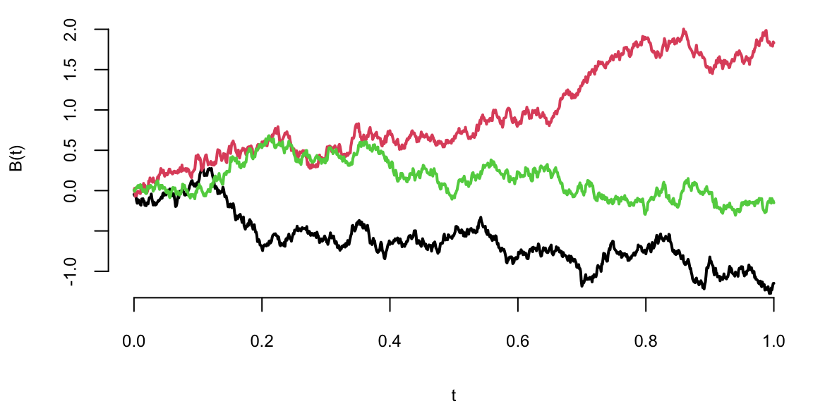
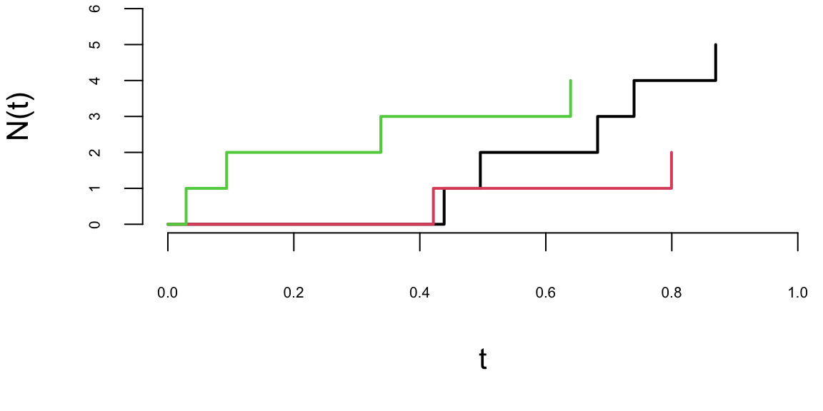
A Poisson process models random events occurring independently at a constant average rate—customer arrivals, call center traffic, or goals in a soccer match. A counting process \(\{N_t, t \geq 0\}\) is a Poisson process with rate \(\lambda > 0\) if:
An equivalent characterization of the Poisson process is through the inter-arrival times between consecutive events. If \(T_1, T_2, \ldots\) denote the times between successive events, then these are independent and identically distributed exponential random variables with mean \(1/\lambda\). This connection between the Poisson and exponential distributions is fundamental: the Poisson process counts events while the exponential distribution models the waiting time between events.
The Poisson process can be viewed from two complementary perspectives. From a continuous-time viewpoint, we track the evolution of the counting process \(N_t\) as time progresses, asking questions about the probability of observing a certain number of events by time \(t\) or the distribution of event times. From a discrete count data perspective, we observe the number of events that occurred during a fixed time interval and use this to make inferences about the underlying rate parameter \(\lambda\).
The connection between these perspectives is crucial for applications. In many real-world scenarios, we observe event counts over fixed intervals (discrete perspective) but need to make predictions about future events or the timing of the next event (continuous perspective). The Poisson process framework unifies these views, allowing us to seamlessly move between counting events and modeling their temporal dynamics.
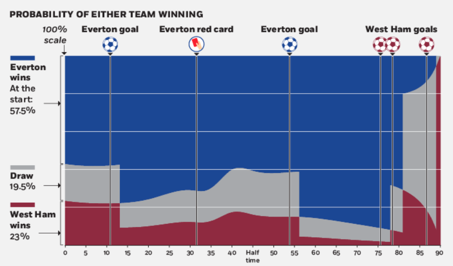
Example 7.4 (EPL Betting) Feng, Polson, and Xu (2016) employ a Skellam process (a difference of Poisson random variables) to model real-time betting odds for English Premier League (EPL) soccer games. Given a matrix of market odds on all possible score outcomes, we estimate the expected scoring rates for each team. The expected scoring rates then define the implied volatility of an EPL game. As events in the game evolve, they re-estimate the expected scoring rates and our implied volatility measure to provide a dynamic representation of the market’s expectation of the game outcome. They use real-time market odds data for a game between Everton and West Ham in the 2015-2016 season. We show how the implied volatility for the outcome evolves as goals, red cards, and corner kicks occur.
Gambling on soccer is a global industry with revenues of over $1 trillion a year (see “Football Betting - the Global Gambling Industry worth Billions,” BBC Sport). Betting on the result of a soccer match is a rapidly growing market, and online real-time odds exist (Betfair, Bet365, Ladbrokes). Market odds for all possible score outcomes (\(0-0, 1-0, 0-1, 2-0, \ldots\)) as well as outright win, lose, and draw are available in real time. In this paper, we employ a two-parameter probability model based on a Skellam process and a non-linear objective function to extract the expected scoring rates for each team from the odds matrix. The expected scoring rates then define the implied volatility of the game.
Skellam Process
To model the outcome of a soccer game between team A and team B, we let the difference in scores, \(N_t = N_{A,t} - N_{B,t}\), where \(N_{A,t}\) and \(N_{B,t}\) are the team scores at time point \(t\). Negative values of \(N_t\) indicate that team A is behind. We begin at \(N(0) = 0\) and end at time one with \(N_1\) representing the final score difference. The probability \(\mathbb{P}(N_1 > 0)\) represents the ex-ante odds of team A winning. Half-time score betting, which is common in Europe, is available for the distribution of \(N_{1/2}\).
Then we find a probabilistic model for the distribution of \(N_1\) given \(N_t = \ell\), where \(\ell\) is the current lead. This model, together with the current market odds, can be used to infer the expected scoring rates of the two teams and then to define the implied volatility of the outcome of the match. We let \(\lambda^A\) and \(\lambda^B\) denote the expected scoring rates for the whole game. We allow for the possibility that the scoring abilities (and their market expectations) are time-varying, in which case we denote the expected scoring rates after time \(t\) by \(\lambda^A_t\) and \(\lambda^B_t\), respectively, instead of \(\lambda^A(1-t)\) and \(\lambda^B(1-t)\).
The Skellam distribution is defined as the difference between two independent Poisson variables given by:
\[
\begin{aligned}
N_{A,t} &= W_{A,t} + W_t \\
N_{B,t} &= W_{B,t} + W_t
\end{aligned}
\]
where \(W_{A,t}\), \(W_{B,t}\), and \(W_t\) are independent processes with:
\[
W_{A,t} \sim \text{Poisson}(\lambda^A t), \quad W_{B,t} \sim \text{Poisson}(\lambda^B t).
\]
Here \(W_t\) is a Poisson process used to induce a correlation between the numbers of goals scored.
\[
N_t = N_{A,t} - N_{B,t} \sim \text{Skellam}(\lambda^A t, \lambda^B t).
\tag{7.2}\]
At time \(t\), we have the conditional distributions:
\[
\begin{aligned}
W_A(1) - W_{A,t} &\sim \text{Poisson}(\lambda^A(1-t)) \\
W_B(1) - W_{B,t} &\sim \text{Poisson}(\lambda^B(1-t)).
\end{aligned}
\]
Now letting \(N^*(1-t)\), the score difference of the sub-game which starts at time \(t\) and ends at time 1 and the duration is \((1-t)\). By construction, \(N_1 = N_t + N^*(1-t)\). Since \(N^*(1-t)\) and \(N_t\) are differences of two Poisson process on two disjoint time periods, by the property of Poisson process, \(N^*(1-t)\) and \(N_t\) are independent. Hence, we can re-express equation (Equation 7.2) in terms of \(N^*(1-t)\), and deduce
\[
%N^*(1-t) = W^*_A(1-t) - W^*_B(1-t) \sim Skellam(\lambda^A (1-t),\lambda^B (1-t) )
N^*(1-t) = W^*_A(1-t) - W^*_B(1-t) \sim \text{Skellam}(\lambda^A_t,\lambda^B_t)
\]
where \(W^*_A(1-t) = W_A(1) - W_{A,t}\), \(\lambda^A = \lambda^A_0\) and \(\lambda^A_t=\lambda^A(1-t)\). A natural interpretation of the expected scoring rates, \(\lambda^A_t\) and \(\lambda^B_t\), is that they reflect the “net” scoring ability of each team from time \(t\) to the end of the game. The term \(W_t\) models a common strength due to external factors, such as weather. The “net” scoring abilities of the two teams are assumed to be independent of each other as well as the common strength factor. We can calculate the probability of any particular score difference, given by \(\mathbb{P}(N_1=x|\lambda^A,\lambda^B)\), at the end of the game where the \(\lambda\)’s are estimated from the matrix of market odds. Team strength and “net” scoring ability can be influenced by various underlying factors, such as the offensive and defensive abilities of the two teams. The goal of our analysis is to only represent these parameters at every instant as a function of the market odds matrix for all scores.
Another quantity of interest is the conditional probability of winning as the game progresses. If the current lead at time \(t\) is \(\ell\), and \(N_t=\ell=N_{A,t}-N_{B,t}\), the Poisson property implied that the final score difference \((N_1|N_t=\ell)\) can be calculated by using the fact that \(N_1=N_t+N^*(1-t)\) and \(N_t\) and \(N^*(1-t)\) are independent. Specifically, conditioning on \(N_t=\ell\), we have the identity
\[ N_1=N_t+N^*(1-t)=\ell+\text{Skellam}(\lambda^A_t,\lambda^B_t). \]
We are now in a position to find the conditional distribution (\(N_1=x|N_t=\ell\)) for every time point \(t\) of the game given the current score. Simply put, we have the time homogeneous condition
\[
\begin{aligned}
\mathbb{P}(N_1=x|\lambda^A_t,\lambda^B_t,N_t=\ell) &= \mathbb{P}(N_1-N_t=x-\ell |\lambda^A_t,\lambda^B_t,N_t=\ell) \\
&= \mathbb{P}(N^* (1-t)=x-\ell |\lambda^A_t,\lambda^B_t)
\end{aligned}
\]
where \(\lambda^A_t\), \(\lambda^B_t\), \(\ell\) are given by market expectations at time \(t\). See Feng et al. for details.
Market Calibration
Our information set at time \(t\) includes the current lead \(N_t = \ell\) and the market odds for \(\{Win, Lose, Draw, Score\}_t\), where \(Score_t = \{ ( i - j ) : i, j = 0, 1, 2, ....\}\). These market odds can be used to calibrate a Skellam distribution which has only two parameters \(\lambda^A_t\) and \(\lambda^B_t\). The best fitting Skellam model with parameters \(\{\hat\lambda^A_t,\hat\lambda^B_t\}\) will then provide a better estimate of the market’s information concerning the outcome of the game than any individual market (such as win odds) as they are subject to a “vig” and liquidity.
Suppose that the fractional odds for all possible final score outcomes are given by a bookmaker. Fractional odds, commonly used in the UK, express the ratio of profit to stake. For example, odds of \(3:1\) (read as “three-to-one”) mean that for every $1 wagered, the bettor receives $3 in profit if the bet wins, plus the original $1 stake returned, for a total payout of $4. In this case, if the bookmaker offers \(3:1\) odds on a 2-1 final score, the bookmaker pays out three times the amount staked by the bettor if the outcome is indeed 2-1. This contrasts with American money-line odds, where positive numbers indicate the profit on a $100 stake (e.g., +300 means $300 profit on $100 wagered), and negative numbers indicate the stake needed to win $100.
The market implied probability makes the expected winning amount of a bet equal to 0. For fractional odds of \(3:1\), the implied probability is calculated as \(p = \frac{1}{1+3} = \frac{1}{4} = 0.25\) or 25%. We can verify this creates a fair bet: the expected winning amount is \(\mu = -1 \times (1-1/4) + 3 \times (1/4) = -0.75 + 0.75 = 0\). We denote these odds as \(odds(2,1) = 3\). To convert all the available odds to implied probabilities, we use the identity
\[ \mathbb{P}(N_A(1) = i, N_B(1) = j)=\frac{1}{1+odds(i,j)}. \]
The market odds matrix, \(O\), with elements \(o_{ij}=odds(i-1,j-1)\), \(i,j=1,2,3...\) provides all possible combinations of final scores. Odds on extreme outcomes are not offered by the bookmakers. Since the probabilities are tiny, we set them equal to 0. The sum of the possible probabilities is still larger than 1 (see Dixon and Coles (1997) and Dixon and Coles (1997)). This “excess” probability corresponds to a quantity known as the “market vig.” For example, if the sum of all the implied probabilities is 1.1, then the expected profit of the bookmaker is 10%. To account for this phenomenon, we scale the probabilities to sum to 1 before estimation.
To estimate the expected scoring rates, \(\lambda^A_t\) and \(\lambda^B_t\), for the sub-game \(N^*(1-t)\), the odds from a bookmaker should be adjusted by \(N_{A,t}\) and \(N_{B,t}\). For example, if \(N_A(0.5)=1\), \(N_B(0.5)=0\) and \(odds(2,1)=3\) at half time, these observations actually says that the odds for the second half score being 1-1 is 3 (the outcomes for the whole game and the first half are 2-1 and 1-0 respectively, thus the outcome for the second half is 1-1). The adjusted \({odds}^*\) for \(N^*(1-t)\) is calculated using the original odds as well as the current scores and given by
\[
{odds}^*(x,y)=odds(x+N_{A,t},y+N_{B,t}).
\]
At time \(t\) \((0\leq t\leq 1)\), we calculate the implied conditional probabilities of score differences using odds information
\[
\mathbb{P}(N_1=k|N_t=\ell)=\mathbb{P}(N^*(1-t)=k-\ell)=\frac{1}{c}\sum_{i-j=k-\ell}\frac{1}{1+{odds}^*(i,j)}
\]
where \(c=\sum_{i,j} \frac{1}{1+{odds}^*(i,j)}\) is a scale factor, \(\ell=N_{A,t}-N_{B,t}\), \(i,j\geq 0\) and \(k=0,\pm 1,\pm 2\ldots\).
Example: Everton vs West Ham (3/5/2016)
Table below shows the implied Skellam probabilities.
Table 7.4 shows the raw data of odds right the game. We need to transform odds data into probabilities. For example, for the outcome 0-0, 11/1 is equivalent to a probability of 1/12. Then we can calculate the marginal probability of every score difference from -4 to 5. We neglect those extreme scores with small probabilities and rescale the sum of event probabilities to one.
Table 7.5 shows the model implied probability for the outcome of score differences before the game, compared with the market implied probability. As we see, the Skellam model appears to have longer tails. Different from independent Poisson modeling in Dixon and Coles (1997), our model is more flexible with the correlation between two teams. However, the trade-off of flexibility is that we only know the probability of score difference instead of the exact scores.
Figure 7.5 examines the behavior of the two teams and represent the market predictions on the final result. Notably, we see the probability change of win/draw/loss for important events during the game: goals scoring and a red card penalty. In such a dramatic game, the winning probability of Everton gets raised to 90% before the first goal of West Ham in 78th minutes. The first two goals scored by West Ham in the space of 3 minutes completely reverses the probability of winning. The probability of draw gets raised to 90% until we see the last-gasp goal of West Ham that decides the game.
Figure 7.5 plots the path of implied volatility throughout the course of the game. Instead of a downward sloping line, we see changes in the implied volatility as critical moments occur in the game. The implied volatility path provides a visualization of the conditional variation of the market prediction for the score difference. For example, when Everton lost a player by a red card penalty at 34th minute, our estimates \(\hat\lambda^A_t\) and \(\hat\lambda^B_t\) change accordingly. There is a jump in implied volatility and our model captures the market expectation adjustment about the game prediction. The change in \(\hat\lambda_A\) and \(\hat\lambda_B\) are consistent with the findings of Vecer, Kopriva, and Ichiba (2009) where the scoring intensity of the penalized team drops while the scoring intensity of the opposing team increases. When a goal is scored in the 13th minute, we see the increase of \(\hat\lambda^B_t\) and the market expects that the underdog team is pressing to come back into the game, an effect that has been well-documented in the literature. Another important effect that we observe at the end of the game is that as goals are scored (in the 78th and 81st minutes), the markets expectation is that the implied volatility increases again as one might expect.
Figure 7.6 compares the updating implied volatility of the game with implied volatilities of fixed \((\lambda^A+\lambda^B)\). At the beginning of the game, the red line (updating implied volatility) is under the “(\(\lambda^A+\lambda^B=4)\)”-blue line; while at the end of the game, it’s above the “(\(\lambda^A+\lambda^B=8)\)”-blue line. As we expect, the value of \((\hat\lambda^A_t + \hat\lambda^B_t)/(1-t)\) in Table 7.6 increases throughout the game, implying that the game became more and more intense and the market continuously updates its belief in the odds.