3 Bayesian Learning

“A Wise man proportions his beliefs to the evidence.”—David Hume

Statistics makes use of parametric families of distributions and often assumes that observed samples $y = (y_1,\ldots,y_n)$ are independent and identically distributed observations from a distribution with density function parametrized by $\theta$, the notation is $y\mid \theta \sim p(y \mid \theta)$. The functional form of $p(y \mid \theta)$ is assumed to be known, but the value of $\theta$ is unknown. The goal of statistical inference is to estimate $\theta$ from the observed data \[ y = (y_1,\ldots,y_n). \]

The main tasks in statistical inference include estimation, hypothesis testing, and prediction. Estimation involves using the observed sample to infer the value of the unknown parameter $\theta$, either by providing a single best guess (denoted as $\hat{\theta}$) or by constructing an interval $[a, b]$ that is likely to contain the true value of $\theta$ with a specified probability. Hypothesis testing focuses on evaluating specific claims or hypotheses about the value of $\theta$; for instance, we might be interested in determining whether $\theta$ is equal to a particular value $\theta_0$. Prediction, on the other hand, is concerned with forecasting the value of a future observation $y_{n+1}$ based on the data already observed, $y_1, \ldots, y_n$ via a model $p(y_{n+1} \mid y_1, \ldots, y_n)$.

In this section, we present a general framework for statistical inference, known as Bayesian inference, which is based on the use of probability distributions to represent uncertainty and make inferences about unknown parameters. We will use Bayes’ rule to update our beliefs about the parameters of a model based on new evidence or data. Bayesian inference provides a principled approach to statistical modeling and decision-making.

Bayesian analysis always starts with specifying the two main components of the model:

Prior $p(\theta)$ represents your beliefs or knowledge about the parameters before observing any data. This distribution encapsulates the uncertainty about the parameters.
Likelihood Function (Data Likelihood): $p(y \mid \theta)$ describes the likelihood of observing the given data given the current values of the parameters. When we have independent and identically distributed $y = (y_1, \ldots, y_n)$, the likelihood function is given by \[ p(y \mid \theta) = \prod_{i=1}^n p(y_i \mid \theta). \]

The estimation problem is also called Bayesian parameter learning; the goal is then to update the probability distribution over the parameters of the model as new data become available. Suppose that you are interested in the values of $k$ unknown quantities \[ \theta = (\theta_1, \ldots, \theta_k). \] Then learning is done by updating the prior distribution over the parameters of the model as new data become available and calculating the posterior distribution over the parameters. The posterior distribution represents the updated beliefs about the parameters after incorporating the observed data. It combines the prior distribution and the likelihood function using Bayes’ theorem: \[ p( \theta \mid y ) = \frac{p(y \mid \theta)p( \theta)}{p(y)} = \frac{\text{Likelihood} \times \text{Prior}}{\text{Marginal}}. \] The left-hand side $p( \theta \mid y )$ is the posterior distribution, and $p(y)$ is the probability of the observed data (also known as the total probability) given by \[ p(y) = \int p(y \mid \theta)p( \theta)d \theta \]

Nice feature of the Bayes approach is that you can use the posterior distribution obtained from one round of observation as the prior distribution for the next round when more data become available. This process can be iteratively repeated as new evidence is acquired. It makes sequential learning possible.

The downstream tasks then use the posterior distribution. For example, if we want to predict the value of a future observation $y_{n+1}$ based on the data already observed, $y_1, \ldots, y_n$ via a model $p(y_{n+1} \mid y_1, \ldots, y_n, \theta)$, we can use the posterior distribution to calculate the expected value of $y_{n+1}$ as \[ p(y_{n+1} \mid y_1, \ldots, y_n) = \int p(y_{n+1} \mid y_1, \ldots, y_n, \theta)p(\theta \mid y_1, \ldots, y_n)d \theta. \] You can think of prediction as a mixture of the conditional distributions $p(y_{n+1} \mid y_1, \ldots, y_n, \theta)$ weighted by the posterior distribution $p(\theta \mid y_1, \ldots, y_n)$.

A simple hypothesis test then involves calculating the probability of the observed data under the null hypothesis $H_0$ as \[ p(y \mid H_0) = \int p(y \mid \theta)p(\theta \mid H_0)d \theta. \]

The downside of the Bayes approach is the requirement to calculate the marginal likelihood $p(y)$, which often requires calculating high-dimensional integrals that are intractable (do not have closed-form solutions). However, often, Bayesian analysis can be performed without calculating the marginal likelihood, in this case, we omit the total probability in the denominator on the right-hand side and write Bayes’ rule as \[ \text{Posterior} \propto \text{Likelihood} \times \text{Prior}. \]

The choice of prior distribution can significantly impact the ease of computation and the interpretation of the posterior distribution. Conjugate priors are a special type of prior distribution that, when combined with a specific likelihood function, result in a posterior distribution that belongs to the same family as the prior. This property simplifies the computation of the posterior distribution, and allows for analytical solutions.

Common examples of conjugate priors include:

Normal distribution with known variance: If the likelihood is a normal distribution with known variance, then a normal distribution is a conjugate prior for the mean.
Binomial distribution: If the likelihood is a binomial distribution, then a beta distribution is a conjugate prior for the probability of success.
Poisson distribution: If the likelihood is a Poisson distribution, then a Gamma distribution is a conjugate prior for the rate parameter.

Using conjugate priors simplifies the Bayesian analysis, especially in cases where analytical solutions are desirable. However, the choice of a conjugate prior is often a modeling assumption, and in some cases, non-conjugate priors may be more appropriate for capturing the true underlying uncertainty in the problem. The blind use of conjugate priors can lead to misleading results. We should never ignore the absence of evidence for use of a specific model.

3.1 Exchangeability and the Bayesian View of Probability Models

At the basis of all statistical problems is a potential sample of data, $y=\left( y_{1},\ldots,y_{T}\right)$, and assumptions over the data generating process such as independence, a model or models, and parameters. How should one view the relationship between models, parameters, and samples of data? How should one define a model and parameters? These questions have fundamental implications for statistical inference and can be answered from different perspectives. We will discuss de Finetti’s representation theorem which provides a formal connection between data, models, and parameters.

To understand the issues, consider the simple example of an experiment consisting of tosses of a simple thumb tack in ideal “laboratory” conditions.¹ The outcome of the experiment can be defined as a random variable $y_{i},$ where $y_{i}=1$ if the $i^{th}$ toss was a heads (the tack lands on the spike portion) and $y_{i}=0$ if the tack lands tails (on its flat portion). How do we model these random variables? The frequentist or objective approach assumes tosses are independent and identically distributed. In this setting, independence implies that \[ P\left( y_{2}=1,y_{1}=1\right) =P\left( y_{2}=1\right) P\left( y_{1}=1\right). \]

Given this, are thumbtack tosses independent? Without conditioning on the unknown parameter $\theta$, the answer is no: observing many heads tells us something about $\theta$, which in turn predicts future tosses. Independence implies that \[ P\left( y_{2}=1 \mid y_{1}=1\right) =P\left( y_{2}=1\right), \] which means that observing $y_{1}=1$ does not affect the probability that $y_{2}=1$. To see the implications of this simple fact, suppose that the results of 500 tosses were available. If the tosses were independent, then \[ P\left( y_{501}=1\right) =P\left( y_{501}=1\mid {\textstyle\sum\nolimits_{t=1}^{500}}y_{t}=1\right) =P\left( y_{501}=1\mid {\textstyle\sum\nolimits_{t=1}^{500}}y_{t}=499\right). \] It is hard to imagine that anyone would believe this–nearly every observer would state that the second probability is near zero and the third probability is near 1, as the first 500 tosses contain a lot of information. Thus, the tosses are not independent.

To see the resolution of this apparent paradox, introduce a parameter, $\theta$, which is the probability that a thumb tack toss is heads. If $\theta$ were known, then it is true that, conditional on the value of this parameter, the tosses are independent and \[ P\left( y_{2}=1\mid y_{1}=1,\theta\right) =P\left(y_{2}=1\mid \theta\right) =\theta. \] Thus, the traditional usage of independence and independent sampling requires that “true” parameter values are known. With unknown probabilities, statements about future tosses are heavily influenced by previous observations, clearly violating the independence assumption. Ironically, if the data were really independent, we would not need samples in the first place to estimate parameters because the probabilities would already be known! Given this, if you were now presented with a thumb tack from a box that was to be repeatedly tossed, do you think that the tosses are independent?

This example highlights the tenuous foundations, an odd circularity, and the internal inconsistency of the frequentist approach that proceeds under the assumption of a fixed “true” parameter. All frequentist procedures are founded on the assumption of known parameter values: sampling distributions of estimators are computed conditional on $\theta$; confidence intervals consist of calculations of the form: $P\left( f\left( y_{1}, \ldots ,y_{T}\right) \in\left( a,b\right) \mid\theta\right)$; and asymptotics also all rely on the assumption of known parameter values. None of these calculations are possible without assuming the known parameters.

In the frequentist approach, even though the parameter is completely unknown to the researcher, $\theta$ is not a random variable, does not have a distribution, and therefore inference is not governed by the rules of probability. Given this “fixed, but unknown” definition, it is impossible to discuss concepts like “parameter uncertainty.” This strongly violates our intuition, since things that are not known are typically thought of as random.

The Bayesian approach avoids this internal inconsistency by shedding the strong assumption of independence and assumption of a fixed but unknown parameter. Instead, it assumes that $\theta$ is a random variable and describes the uncertainty about $\theta$ using a probability distribution, $p\left( \theta\right)$ (the prior). The joint distribution of the data is then \[ p(y_{1}, \ldots ,y_{T}) = \int p(y_{1}, \ldots ,y_{T} \mid \theta) p(\theta)d\theta = \int\prod_{t=1}^Tp(y_t\mid \theta) p( \theta)d\theta. \] Notice that the right-hand-side does not depend on the order of the data, and the joint distribution of the data is the same for all potential orderings. This is a natural assumption about the symmetry of the data, and is called exchangeability. The Bayesian approach makes no assumptions about the order in which the data may arrive, and each observation has the same marginal distribution, $P\left( y_{i}=1\right) =P\left(y_{j}=1\right)$ for any $i$ and $j$.

Thus, we replace the independence assumption with a weaker and more natural assumption of exchangeability: a collection of random variables, $y_{1}, \ldots ,y_{T}$, is exchangeable if the distribution of $y_{1}, \ldots ,y_{T}$ is the same as the distribution of any permutation $y_{\pi_{1}}, \ldots ,y_{\pi_{T}}$, where $\pi=\left( \pi_{1}, \ldots ,\pi_{T}\right)$ is a permutation of the integers $1$ to $T$. Independent events are always exchangeable, but the converse is not true. Notice the differences between the assumptions in the Bayesian and frequentist approach: the Bayesian makes assumptions over potentially realized data, and there is no need to invent the construct of a fixed but unknown parameter, since exchangeability makes no reference to parameters.

In the case of the tack throwing experiment, exchangeability states that the ordering of heads and tails does not matter. Thus, if the experiment of 8 tosses generated 4 heads, it does not matter if the ordering was $\left(1,0,1,0,1,0,1,0\right)$ or $\left( 0,1,1,0,1,0,0,1\right)$. This is a natural assumption about the symmetry of the tack tosses, capturing the idea that the information in any toss or sequence of tosses is the same as any other–the idea of a truly random sample. It is important to note that exchangeability is a property that applies prior to viewing the data. After observation, data are no longer random variables, but realizations of random variables.

Bruno de Finetti introduced the notion of exchangeability, and then asked a simple question: “What do exchangeable sequences of random variables look like?” The answer to this question is given in the famous de Finetti’s theorem, which also defines models, parameters, and provides important linkages between frequentist and classical statistics.

de Finetti’s Representation Theorem

de Finetti’s representation theorem provides the theoretical connection between data, models, and parameters. It is stated first in the simplest setting, where the observed data take two values, either zero or one, and then extended below.

Theorem 3.1 (de Finetti’s Representation Theorem) Let $\left( Y_{1},Y_{2},\ldots\right)$ be an infinite sequence of 0-1 exchangeable random variables with joint density $p\left(Y_{1}, \ldots ,Y_{n}\right)$. Then there exists a distribution $P$ such that \[ P(Y_{1}=y_1,\ldots,Y_{n}=y_n)=\int\prod_{i=1}^{n}\theta^{y_{i}}(1-\theta)^{1-y_{i}}dP(\theta)=\int\prod_{i=1}^{n}p\left( y_{i} \mid \theta\right) dP(\theta) \tag{3.1}\] where \[ P(\theta)=\lim_{n\rightarrow\infty}\text{Prob}\left[ \frac{1}{n}\sum_{t=1}^{n}Y_{t}\leq\theta\right] \text{ and }\theta=\lim_{n\rightarrow\infty}\frac{1}{n}\sum_{t=1}^{n}Y_{t}. \] If the distribution function or measure admits a density with respect to Lebesgue measure, then $dP(\theta)=p\left( \theta\right) d\theta$.

Heath and Sudderth (1976) provide a general version and simple proof. For general spaces $\mathcal{Y}$, we have \[ P(Y_1 \le y_1, \ldots, Y_n \le y_n) = \int_{\mathcal{F}} \prod_{i=1}^{n} F(y_i) \, \mu(dF) \] where $\mu(\cdot)$ is a measure over the space of distributions, $\mathcal{F}$. In the parametric case, $F_\theta$, then $\mu(d\theta) = p(\theta) d\theta$ and $p(\theta)$ is the typical prior density. The predictive $p(Y_{n+1} \mid y_1, \ldots, y_n)$ is then a marginal over $F_\theta$ and the posterior $p(\theta \mid y_1, \ldots, y_n)$ which is updated via Bayes’ theorem.

de Finetti’s representation theorem has deep implications for understanding models from a subjectivist perspective and in relating subjectivist to frequentist theories of inference. The theorem is interpreted as follows:

Under exchangeability, parameters exist, and one can act as if the $y_{i}$’s are drawn independently from a Bernoulli distribution with parameter $\theta$. That is, they are draws from the model $p\left(y_{i} \mid \theta\right) =\theta^{y_{i}}(1-\theta)^{1-y_{i}},$ generating a likelihood function $p\left( y \mid \theta\right) =\prod_{i=1}^{n}p\left(y_{i} \mid \theta\right)$. Formally, the likelihood function is defined via the density $p\left( y \mid \theta\right)$, viewed as a function of $\theta$ for a fixed sample $y=\left( y_{1}, \ldots ,y_{n}\right)$. More "likely" parameter values generate higher likelihood values, thus the name. The maximum likelihood estimate (MLE) is \[ \widehat{\theta}_{\mathrm{MLE}}=\arg\underset{\theta\in\Theta}{\max}\text{ }p\left(y \mid \theta\right) =\arg\underset{\theta\in\Theta}{\max}\ln p\left(y \mid \theta\right), \] where $\Theta$ is the parameter space.
Parameters are random variables. The limit $\theta=\underset {n\rightarrow\infty}{\lim}n^{-1}\sum_{i=1}^{n}y_{i}$ exists but is a random variable. This can be contrasted with the strong law of large numbers that requires independence and implies that $n^{-1}\sum_{i=1}^{n}y_{i}$ converges almost surely to a fixed value, $\theta_{0}$. From this, one can interpret a parameter $\theta$ as a limit of observables and justifies the frequentist interpretation of $\theta$ as a limiting frequency of 1’s.
The distribution $P\left( \theta\right)$ or density $p\left(\theta\right)$ can be interpreted as beliefs about the limiting frequency $\theta$ prior to viewing the data. After viewing the data, beliefs are updated via Bayes’ rule resulting in the posterior distribution, $p(\theta \mid y_{1},\ldots,y_{n})$.

Since the likelihood function is fixed in this case, any distribution of observed data can be generated by varying the prior distribution.

The main implication of de Finetti’s theorem is a complete justification for Bayesian practice of treating the parameters as random variables and specifying a likelihood and parameter distribution. Stated differently, a “model” consists of both a likelihood and a prior distribution over the parameters. Thus, parameters as random variables and priors are a necessity for statistical inference, and not some extraneous component motivated by philosophical concerns.

More general versions of de Finetti’s theorem are available. A general version is as follows. If $\left\{ Y_{i}\right\} _{i\geq1}$, $Y_{i}\in\mathbb{R}$, is a sequence of infinitely exchangeable random variables, then there exists a probability measure $P$ on the space of all distribution functions, such that \[ p(Y_{1}\le y_{1},\ldots,Y_{n}\le y_{n})=\int\prod_{i=1}^{n}F\left( y_{i}\right) P(dF) \] with mixing measure \[ P\left( F\right) =\underset{n\rightarrow\infty}{\lim}P(F_{n}), \] where $F_{n}$ is the empirical distribution of the data. At this level of generality, the distribution function is infinite-dimensional. In practice, additional subjective assumptions are needed that usually restrict the distribution function to finite-dimensional spaces, which implies that the distribution function is indexed by a parameter vector $\theta$: \[ p(Y_{1}\le y_{1},\ldots,Y_{n}\le y_{n})=\int\prod_{i=1}^{n}p\left( Y_{i} \mid \theta\right) dP\left( \theta\right). \] To operationalize this result, the researcher needs to choose the likelihood function and the prior distribution of the parameters.

Posterior Empirical CDF

Let $m = \{ f_\theta ( y ) : y \in \mathcal{Y} \}$ be a model. When necessary we index the parameters in model $m$, as $\theta_m$. Let $y = ( y_1 , \ldots , y_n )$ be a vector of signals. The conditional likelihood, under $m$, is given by $f_\theta(y) = \prod_{i=1}^n f_\theta ( y_i )$. We also allow for the possibility that the data are generated from a model $f$ that does not belong to the family of models $f_\theta$.

Given a prior measure, $\Pi ( d F )$, over $\mathcal{F}$ the set of distributions, we can calculate the predictive density \[ f_n ( y_{n+1} | y_1 , \ldots , y_n ) = \int f (y) \Pi_n ( d F ) \; \text{where}\; \Pi_n ( d f ) = \frac{ \prod_{i=1}^n f( y_i ) \Pi( d f ) }{ \int \prod_{i=1}^n f( y_i ) \Pi( d f ) } \] Under the family, $f_\theta$, we can calculate the parameter posterior as \[ p( \theta \mid y ) = \frac{ \prod_{i=1}^n f_\theta ( y_i ) p(\theta) d \theta }{ m(y) } \; \text{where}\; m(y) = \int f_\theta (y) p( \theta ) d \theta \] Here $p(\theta)$ is a prior distribution over parameters and $m(y)$ is the marginal distribution of the data implied by the model. There are many applications in Bayesian non-parametric statistics.

At first glance, de Finetti’s theorem may seem to suggest that there is a single model or likelihood function. This is not the case however, as models can be viewed in the same manner as parameters. Denoting a model specification by $\mathcal{M}$, then de Finetti’s theorem would imply that \[\begin{align*} p(y_{1},\ldots,y_{n}) & =\int\prod_{i=1}^{n}p\left( y_{i} \mid \theta ,\mathcal{M}\right) p\left( \theta \mid \mathcal{M}\right) p\left(\mathcal{M}\right) d\theta d\mathcal{M}\\ & =\int p(y_{1},\ldots,y_{n} \mid \mathcal{M})p\left( \mathcal{M}\right) d\mathcal{M}, \end{align*}\] in the case of a continuum of models. Thus, under the mild assumption of exchangeability, it is as if the $y_{i}$’s are generated from $p\left( y_{i} \mid \theta,\mathcal{M}\right)$, conditional on the random variables $\theta$ and $\mathcal{M}$, where $p\left( \theta \mid \mathcal{M}\right)$ are the beliefs over $\theta$ in model $\mathcal{M}$, and $p\left(\mathcal{M}\right)$ are the beliefs over model specifications.

Subjective probability is a more general definition of probability than the frequentist definition, as it can be used for all types of events, both repeatable and unrepeatable events. A subjectivist has no issues discussing the probability of an election result, even though the underlying conditions has not been observed before. As Ramsey (1926) frames it, probability is simply one’s willingness to bet on an event with a counterparty.

The event does not even have to be uncertain in nature. For example, the probability of me having coins in my pocket will depend on who is asked to make the assessment. I, knowing the contents of my pocket, will say the probability is 0. However, if you are asked to make the assessment, you will say the probability is 1/2, as you do not know the contents of my pocket. This is a classic example of subjectivist probability.

Similarly, consider the number of people currently in Antarctica. This number is fixed and deterministic at any given moment, yet different individuals will assign different probability distributions to this quantity based on their knowledge. A researcher who recently reviewed Antarctic population statistics might have a tight distribution centered around the correct value, while someone with no such knowledge might have a much wider distribution. A logistics coordinator for a polar research station would have precise information about personnel at their specific facility but uncertainty about other stations. Each of these represents valid subjective probabilities over the same underlying fixed quantity, illustrating how probability in the Bayesian sense quantifies personal uncertainty rather than intrinsic randomness.

The main difficulty in operationalizing subjective probability is the process of actually quantifying subjective beliefs into numeric probabilities. One practical approach is to elicit probabilities through a sequence of carefully designed bets.

Consider eliciting someone’s probability distribution over the number of people in Antarctica. We could start by asking: “Would you accept a bet that pays $100 if the number is below 5,000, and you pay $50 if it’s above 5,000?” If they accept, this suggests they believe $P(\text{population} < 5000) > 1/3$. We then adjust the threshold and payoffs systematically. For instance, we might ask about betting on the population being below 2,000, or below 1,000, gradually narrowing down probability mass at different intervals.

For continuous quantities, we can elicit a full distribution through a sequence of binary bets about quantiles. By asking someone to specify values $q_{0.25}, q_{0.5}, q_{0.75}$ such that they are indifferent between bets paying equal amounts if the true value falls below or above each threshold, we construct their 25th, 50th, and 75th percentiles. This process, known as probability elicitation, transforms abstract beliefs into concrete probability distributions by observing revealed preferences through betting behavior.

The betting framework provides two key advantages. First, it forces coherence: if someone states inconsistent probabilities (such as $P(A) + P(\neg A) \neq 1$), an adversary could construct a Dutch book—a set of bets that guarantees a loss regardless of the outcome. The threat of sure loss incentivizes rational probability assignments. Second, betting naturally handles non-repeatable events. We can elicit probabilities about tomorrow’s Supreme Court decision or next quarter’s GDP growth, neither of which has a frequentist interpretation.

Instead of using repetitive experiments, subjective probabilities can be measured using betting odds, which have been used for centuries to gauge the uncertainty over an event. The probability attributed to winning a coin toss is revealed by the type of odds one would accept to bet. Notice the difference between the frequentist and Bayesian approach. Instead of defining the probabilities via an infinite repeated experiment, the Bayesian approach elicits probabilities from an individual’s observed behavior.

3.2 Sufficient Statistic

In Bayesian inference, we need to compute the posterior over unknown model parameters $\theta$, given data $y$. The posterior density is denoted by $p(\theta \mid y)$. A map from data $y = (y_1, \ldots, y_n)$ to a statistic $S(y)$ is called a sufficient statistic for $\theta$ if the conditional distribution of $y$ given $S(y)$ is independent of $\theta$: \[ p(y\mid S(y),\theta) = p(y\mid S(y)). \] This implies that $S(y)$ captures all the information in the data relevant to $\theta$. Because the statistic is a deterministic function of the data, the likelihood factorizes as: \[ p(y\mid \theta) = p(S(y)\mid \theta)p(y\mid S(y)). \]

There is a deep connection between the posterior mean and sufficient statistics in the exponential family. Kolmogorov (1942) showed that if $S^*(y)$ is a minimal sufficient statistic, then the posterior expectation $\E{\theta \mid y}$ is a function of $S^*(y)$. This provides a theoretical foundation for using summary statistics in simplified models.

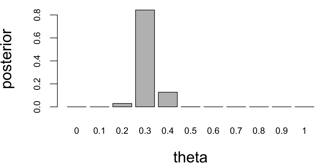
Example 3.1 (Posterior Distribution for Coin Toss) What if we gamble against unfair coin flips or the person who performs the flips is trained to get the side he wants? In this case, we need to estimate the probability of tails $\theta$ from the data. Suppose we have observed 10 flips \[ \{H, T, H, H, H, T, H, T, H, H\}, \] and only three of them were tails. What is the probability that the next flip will be tail? The frequency-based answer would be $3/10 = 0.3$. However, the Bayes approach gives us more flexibility. Suppose we have a prior belief that the coin is fair, but we are not sure. We model this belief by a prior distribution. Let’s discretize the variable $\theta$ and assign prior probabilities to each value of $\theta$, the prior distribution is shown in Figure 3.1 (left panel).

theta <- seq(0, 1, by = 0.1)
prior <- c(0, 0.024, 0.077, 0.132, 0.173, 0.188, 0.173, 0.132, 0.077, 0.024, 0)

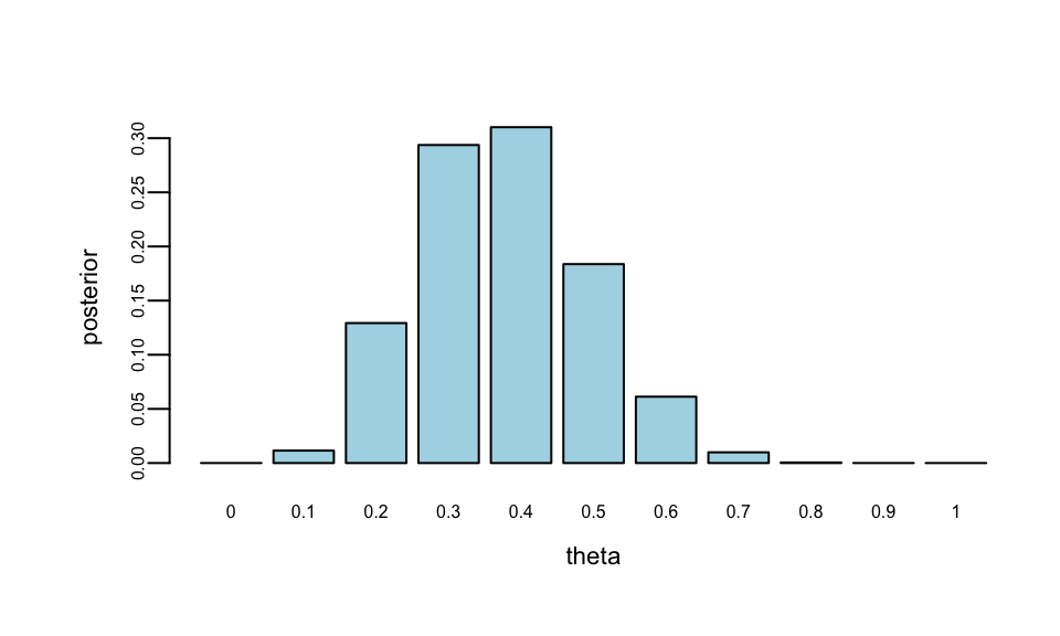
We put most of the mass on the fair assumption ($\theta = 0.5$) and zero mass on the extreme values $\theta = 0$ and $\theta = 1$. Our mass is exponentially decaying as we move away from 0.5. This is a reasonable assumption, since we are not sure about the fairness of the coin. Now, we can use Bayes’ rule to update our prior belief. The posterior distribution then combines the likelihood shown in Figure 3.1 (middle panel) and the prior distribution as shown in Figure 3.1 (right panel). \[ p(\theta \mid y) = \frac{p(y \mid \theta) p(\theta)}{p(y)}. \] The denominator is the marginal likelihood, which is given by \[ p(y) = \sum_{\theta} p(y \mid \theta) p(\theta). \] The likelihood is given by the Binomial distribution \[ p(y \mid \theta) \propto \theta^3 (1 - \theta)^7. \] Notice that the posterior distribution depends only on the number of positive and negative cases. Those numbers are sufficient for the inference about $\theta$.

par(mar = c(4, 4, 3, 1))
barplot(prior, names.arg = theta, xlab = "theta", ylab = "prior", col = "lightblue")

likelihood <- function(theta, n, Y) {
  theta^Y * (1 - theta)^(n - Y)
}
posterior <- likelihood(theta, 10, 3) * prior
posterior <- posterior / sum(posterior) # normalize
barplot(posterior, names.arg = theta, xlab = "theta", ylab = "posterior", col = "lightblue")

posterior <- likelihood(theta, 100, 30) * prior
posterior <- posterior / sum(posterior) # normalize
barplot(posterior, names.arg = theta, xlab = "theta", ylab = "posterior", col = "lightblue")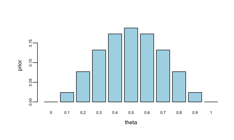

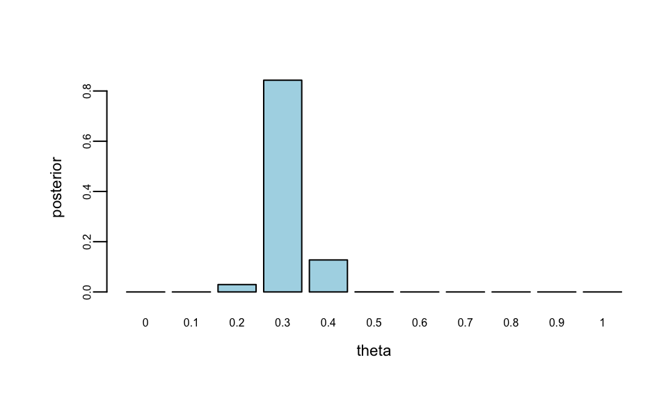
If you are to keep collecting more observations and say observe a sequence of 100 flips and 30 of them were tails, then the posterior distribution will be more concentrated around the value of $\theta = 0.3$, as shown in Figure 3.1 (right panel).

This demonstrates that for large sample sizes, the frequentist approach and the Bayesian approach agree.

3.3 Beta-Binomial Model

The Beta-Binomial Bayesian model is a statistical model that is used when we are interested in learning about a proportion or probability of success, denoted by $p$. This model is used, for example, when dealing with binary data in A/B testing.

In the Beta-Binomial model, we assume that the observed data are generated from a Binomial distribution with parameter $\theta$ and $m$ trials. The probability of success $\theta$ in each of $m$ Bernoulli trials is not fixed but randomly drawn from a Beta distribution. Thus, the model is given by \[ y_i \mid \theta \sim Binomial(m,\theta) ~\text{(likelihood)}, \quad \theta \sim Beta(\alpha,\beta) ~\text{(prior)}. \]

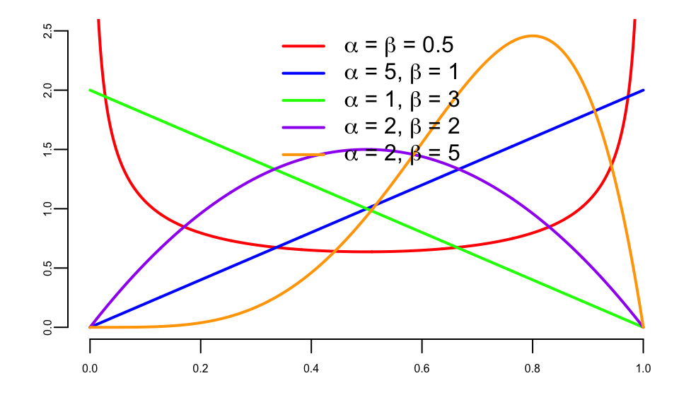
The Beta distribution is a family of continuous probability distributions defined on the interval [0,1] and has two parameters, alpha ($\alpha$) and beta ($\beta$), that appear as exponents of the variable and its complement to 1, respectively, and control the shape of the distribution. The Beta distribution is frequently used in Bayesian statistics, empirical Bayes methods, and classical statistics to model random variables with values falling inside a finite interval.

The probability density function (PDF) of the Beta distribution is given by: \[ Beta(y; \alpha, \beta) = \frac{y^{\alpha - 1}(1 - y)^{\beta - 1}}{B(\alpha, \beta)} \] where $y \in [0, 1]$, $\alpha > 0$, $\beta > 0$, and $B(\alpha, \beta)$ is the beta function. It is simply a normalizing constant \[ B\left( \alpha,\beta\right) =\int_{0}^{1}y^{\alpha-1}\left( 1-y\right)^{\beta-1}dy . \]

The mean and variance of the Beta distribution are given by: \[ \begin{aligned} \mu &= \frac{\alpha}{\alpha + \beta} \\ \sigma^2 &= \frac{\alpha\beta}{(\alpha + \beta)^2(\alpha + \beta + 1)} \end{aligned} \] where $\mu$ is the mean and $\sigma^2$ is the variance.

Figure 3.2 illustrates the Beta distribution for different values of $\alpha$ and $\beta$.

The Beta-Binomial model is one of the simplest Bayesian models and is widely used in various fields including epidemiology, intelligence testing, and marketing. It provides the tools we need to study the proportion of interest, $\theta$, in a variety of settings.

The nice property of the Beta-Binomial model is that the posterior \[ p(\theta \mid y) = \dfrac{p(y \mid \theta)p(\theta)}{p(y)} \] $p(\theta\mid y)$ is yet another Beta distribution. Beta is called a conjugate prior for the Binomial likelihood and is a very useful property.

Conjugate Prior

A prior is called a conjugate prior for a likelihood function if the posterior distribution is of the same family as the prior distribution.

When $m=1$ (observations follow the Bernoulli distribution), the posterior is given by \[ p(\theta\mid Y) = Beta(Y+\alpha, n-Y+\beta) \] where $Y$ is the number of successful outcomes \[ Y = \sum_{i=1}^n y_i, \] where $y_i \mid \theta \sim Bernoulli(\theta)$.

Here the count of successful outcome $Y$ acts as a sufficient statistic for the parameter $\theta$. This means that the posterior distribution depends on the data only through the sufficient statistic $Y$. This is a very useful property and is a consequence of the conjugacy of the Beta prior and Binomial likelihood.

In the general case where each observation follows a Binomial distribution with $m$ trials, i.e., $y_i \mid \theta \sim Binomial(m,\theta)$, the total number of successes is \[ Y = \sum_{i=1}^n y_i, \] and the posterior is \[ \theta\mid Y \sim Beta(Y+\alpha, nm-Y+\beta), \] where $n$ is the number of observations and $nm$ is the total number of Bernoulli trials.

The posterior mean and variance are \[ \E{\theta\mid Y} =\frac{\alpha_{n}}{\alpha_{n}+\beta_{n}} \;\text{ and }\; \Var{ \theta\mid Y} =\frac{\alpha_{n}\beta_{n}}{\left( \alpha_{n}+\beta_{n}\right) ^{2}\left( \alpha_{n}+\beta_{n}+1\right) }\text{,} \] where $\alpha_{n} = \alpha + Y$ and $\beta_{n} = \beta + n - Y$.

Example 3.2 (Black Swans) A related problem is the Black Swan inference problem. Suppose that after $n$ trials, where $n$ is large, you have only seen successes and that you assess the probability of the next trial being a success as $(T+1)/(T+2)$, that is, almost certain. This is a model of observing White Swans and having never seen a Black Swan. Taleb (2007) makes it sound as if the rules of probability are not rich enough to be able to handle Black Swan events. There is a related class of problems in finance known as Peso problems where countries decide to devalue their currencies, and there is little prior evidence from recent history that such an event is going to happen.

To obtain such a probability assessment, we use a Binomial/Beta conjugate Bayes updating model. The key point is that it can also explain that there is still a large probability of a Black Swan event to happen sometime in the future. An independence model has difficulty doing this.

The Bayes Learning Beta-Binomial model will have no problem. We model with $y_{t}=0$ or $1$, with probability $P\left( y_{t}=1\mid \theta\right) =\theta$. This is the classic Bernoulli “coin-flipping” model and is a component of more general specifications such as regime switching or outlier-type models.

Let $Y = \sum_{t=1}^{T}y_{t}$ be the number of observed successful outcomes. The likelihood for a sequence of Bernoulli observations is then \[ p\left( y\mid \theta\right) =\prod_{t=1}^{T}p\left( y_{t}\mid \theta\right) =\theta^{Y}\left( 1-\theta\right)^{T-Y}. \] The maximum likelihood estimator is the sample mean, $\widehat{\theta} = T^{-1}Y$. This makes little sense when you just observe white swans. It predicts $\hat{\theta} = 1$ and gets shocked when it sees a black swan (zero probability event). Bayes, on the other hand, allows for “learning”.

Bayes’ rule then tells us how to combine the likelihood and prior to obtain a posterior distribution, namely $\theta \mid Y=y$. What do we believe about $\theta$ given a sequence of observations? By conjugacy (see Exercise 3.1), the posterior distribution is again a Beta distribution with \[ p\left( \theta\mid y\right) \sim Beta\left( \alpha_{n},\beta_{n}\right) \; \mathrm{ and} \; \alpha_{n}=\alpha+Y , \beta_{n}=\beta+T-Y. \]

Suppose we have observed $T=100$ white swans and no black swans ($Y=100$). Using a uniform prior $Beta(1,1)$, the posterior is $Beta(101,1)$. The predictive probability that the next swan is white is the posterior mean: \[ P(y_{T+1} = 1 \mid Y=100) = \E{\theta \mid Y} = \frac{\alpha_n}{\alpha_n + \beta_n} = \frac{101}{102} \approx 0.99. \] What about the probability of seeing at least one black swan in the next 100 observations? We compute this by integrating over the posterior: \[ P(\text{at least one black swan in next } 100 \mid Y) = \int_0^1 \left[1 - \theta^{100}\right] p(\theta \mid Y) d\theta. \]

## P(next swan is white) = 0.99
## P(at least one black swan in next 100) = 0.5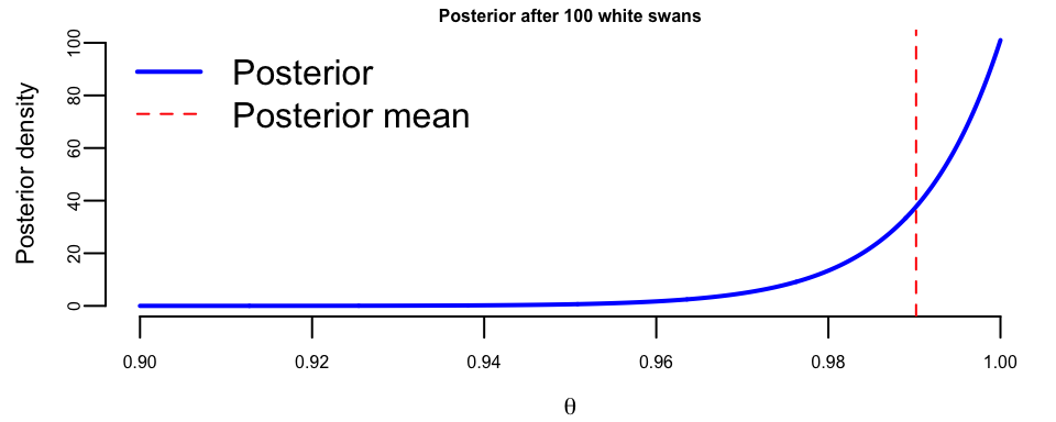

Figure 3.3: Posterior distribution after observing 100 white swans.

Despite never having observed a black swan, the Bayesian approach assigns approximately 49.9% probability to seeing at least one black swan in the next 100 trials. This illustrates how Bayesian learning naturally handles rare events by maintaining uncertainty about $\theta$ through the posterior distribution.

Example 3.3 (Clinical Trials) Consider a problem of designing clinical trials in which $K$ possible drugs $a\in 1,\dots,K$ need to be tested. The outcome of the treatment with drug $a$ is binary $y(a) \in \{0,1\}$. We use Bernoulli distribution with mean $f(a)$ to model the outcome. Thus, the full probabilistic model is described by $w = f(1),\dots,f(K)$. Say we have observed a sample $D = \{y_1,\dots,y_n\}$. We would like to compute posterior distribution over $w$. We start with a Beta prior \[ p(w\mid \alpha,\beta) = \prod_{a=1}^K Beta(w_a\mid \alpha,\beta) \] Then the posterior distribution is given by \[ p(w\mid D) = \prod_{a=1}^K Beta(w_a\mid \alpha + n_{a,1},\beta + n_{a,0}) \]

This setup allows us to perform sequential design of experiments. The simplest version of it is called Thompson sampling. After observing $n$ patients, we draw a single sample $\tilde w$ from the posterior and then maximize the resulting surrogate \[ a_{n+1} = \arg\max_{a} f_{\tilde w}(a), ~~~ \tilde{w} \sim p(w\mid D) \]

Example 3.4 (Shrinkage and Baseball Batting Averages) The batter-pitcher match-up is a fundamental element of a baseball game. There are detailed baseball records that are examined regularly by fans and professionals. These data provide a good illustration of Bayesian hierarchical methods. There is a great deal of prior information concerning the overall ability of a player. However, we only see a small amount of data about a particular batter-pitcher match-up. Given the relatively small sample size, to determine our optimal estimator, we build a hierarchical model taking into account the within pitcher variation.

Let’s analyze the variability in Jeter’s $2006$ season. Let $p_{i}$ denote Jeter’s ability against pitcher $i$ and assume that $p_{i}$ varies across the population of pitchers according to a particular probability distribution $(p_{i} \mid \alpha,\beta)\sim Be(\alpha,\beta)$. To account for extra-binomial variation, we use a hierarchical model for the observed number of hits $y_{i}$ of the form \[ (y_{i} \mid p_{i})\sim Bin(T_{i},p_{i})\;\;\mathrm{with}\;\;p_{i}\sim Be(\alpha,\beta) \] where $T_{i}$ is the number of at-bats against pitcher $i$. A priori we have a prior mean given by $\E{p_{i}}=\alpha/(\alpha+\beta)=\bar{p}$. The extra heterogeneity leads to a prior variance $\Var{p_{i}}=\bar{p}(1-\bar{p})\phi$ where $\phi=(\alpha+\beta+1)^{-1}$. Hence $\phi$ measures how concentrated the beta distribution is around its mean, $\phi=0$ means highly concentrated and $\phi=1$ means widely dispersed.

This model assumes that each player $i$ has a true ability $p_{i}$ that is drawn from a common distribution. The model is hierarchical in the sense that the parameters $\alpha$ and $\beta$ are estimated from the data. The model is also a shrinkage model in the sense that the estimates of $p_{i}$ are shrunk towards the overall mean $\bar{p}_{i}$. In reality, we don’t know that each $p_i$ exists. We also don’t know if it follows a Binomial distribution with the Beta prior. We are making a model assumption. However, the model is a good approximation to the data and is a good way to estimate the parameters.

Stern et al. (2007) estimates the parameter $\hat{\phi} = 0.002$ for Derek Jeter, showing that his ability varies a bit but not very much across the population of pitchers. The effect of the shrinkage is not surprising. The extremes are shrunk the most, with the highest degree of shrinkage occurring for the match-ups that have the smallest sample sizes. The amount of shrinkage is related to the large amount of prior information concerning Jeter’s overall batting average. Overall Jeter’s performance is extremely consistent across pitchers, as seen from his estimates. Jeter had a season $.308$ average. We see that his Bayes estimates vary from $.311$ to $.327$ and that he is very consistent. If all players had a similar record, then the assumption of a constant batting average would make sense.

Pitcher	At-bats	Hits	ObsAvg	EstAvg	95% Int
R. Mendoza	6	5	.833	.322	(.282, .394)
H. Nomo	20	12	.600	.326	(.289, .407)
A.J.Burnett	5	3	.600	.320	(.275, .381)
E. Milton	28	14	.500	.324	(.291, .397)
D. Cone	8	4	.500	.320	(.218, .381)
R. Lopez	45	21	.467	.326	(.291, .401)
K. Escobar	39	16	.410	.322	(.281, .386)
J. Wettland	5	2	.400	.318	(.275, .375)
T. Wakefield	81	26	.321	.318	(.279, .364)
P. Martinez	83	21	.253	.312	(.254, .347)
K. Benson	8	2	.250	.317	(.264, .368)
T. Hudson	24	6	.250	.315	(.260, .362)
J. Smoltz	5	1	.200	.314	(.253, .355)
F. Garcia	25	5	.200	.314	(.253, .355)
B. Radke	41	8	.195	.311	(.247, .347)
D. Kolb	5	0	.000	.316	(.258, .363)
J. Julio	13	0	.000	.312	(.243, .350 )
Total	6530	2061	.316

Some major league managers believe strongly in the importance of such data (Tony La Russa, Three days in August). One interesting example is the following. On Aug 29, 2006, Kenny Lofton (career $.299$ average, and current $.308$ average for $2006$ season) was facing the pitcher Milton (current record $1$ for $19$). He was rested and replaced by a $.273$ hitter. Is putting in a weaker player really a better bet? Was this just an over-reaction to bad luck in the Lofton-Milton match-up? Statistically, from Lofton’s record against Milton we have $P\left( \leq 1\;\mathrm{hit\;in}\ 19\;\mathrm{attempts} \mid p=0.3\right) =0.01$ an unlikely $1$-in-$100$ event. However, we have not taken into account the multiplicity of different batter-pitcher match-ups. We know that Lofton’s batting percentage will vary across different pitchers, it’s just a question of how much? A hierarchical analysis of Lofton’s variability gave a $\phi=0.008$—four times larger than Jeter’s $\phi=0.002$. Lofton has batting estimates that vary from $.265$ to $.340$, with the lowest being against Milton. Hence, the optimal estimate for a pitch against Milton is $.265<.275$ and resting Lofton against Milton is justified by this analysis.

3.4 Poisson Model for Count Data

The Poisson distribution is obtained as a result of the Binomial when $p$ is small and $n$ is large. In applications, the Poisson models count data. Suppose we want to model the arrival rate of users to one of our stores. Let $\lambda = np$, which is fixed and take the limit as $n \rightarrow \infty$. There is a relationship between $p(x)$ and $p(x+1)$ given by \[ \dfrac{p(x+1)}{p(x)}= \dfrac{\left(\dfrac{n}{x+1}\right)p^{x+1}(1-p)^{n-x-1}}{\left(\dfrac{n}{x}\right)p^{x}(1-p)^{n-x}} \approx \dfrac{np}{x+1} \] If we approximate $p(x+1)\approx \lambda p(x)/(x+1)$ with $\lambda=np$, then we obtain the Poisson pdf given by $p(x) = p(0)\lambda^x/x!$. To ensure that $\sum_{x=0}^\infty p(x) = 1$, we set \[ f(0) = \dfrac{1}{\sum_{x=0}^{\infty}\lambda^x/x!} = e^{-\lambda}. \] The above equality follows from the power series property of the exponent function \[ e^{\lambda} = \sum_{x=0}^{\infty}\dfrac{\lambda^x}{x!} \] The Poisson distribution counts the occurrence of events. Given a rate parameter, denoted by $\lambda$, we calculate probabilities as follows \[ p( X = x ) = \frac{ e^{-\lambda} \lambda^x }{x!} \; \mathrm{ where} \; x=0,1,2,3, \ldots \] For $n$ independent Poisson observations $x_1,\ldots,x_n$, the sufficient statistic for $\lambda$ is the sum $\sum_{i=1}^n x_i$. The mean and variance of the Poisson are given by:

Poisson Distribution	Parameters
Expected value	$\mu = \E{X} = \lambda$
Variance	$\sigma^2 = \Var{X} = \lambda$

Here $\lambda$ denotes the rate of occurrence of an event.

Consider the problem of modeling soccer scores in the English Premier League (EPL) games. We use data from Betfair, a website which posts odds on many football games. The goal is to calculate odds for the possible scores in a match. \[ 0-0, \; 1-0, \; 0-1, \; 1-1, \; 2-0, \ldots \]

Another question we might ask, is what’s the odds of a team winning? This is given by $P\left ( X> Y \right )$. The odds of a draw are given by $P \left ( X = Y \right )$. Here $X$ is the number of goals scored by the home team, and $Y$ is the number of goals scored by the away team.

Professional sports bettors rely on sophisticated statistical models to predict the outcomes. Instead, we present a simple but useful model for predicting outcomes of EPL games. We follow the methodology given in Spiegelhalter and Ng (2009).

To make the discussion more concrete, we will use data from the English Premier League (EPL) 2014/2015 season and model the game between Manchester United and Hull City.

First, load the data and then model the number of goals scored using Poisson distribution for each team.

home_team_name	away_team_name	home_score	guest_score
Arsenal	Liverpool	3	4
Bournemouth	Manchester United	1	3
Burnley	Swansea	0	1
Chelsea	West Ham	2	1
Crystal Palace	West Bromwich Albion	0	1
Everton	Tottenham	1	1

Let’s compare the empirical distribution across the number of goals scored by Manchester United to the Poisson distribution.

Histogram vs Poisson Model Prediction of Goals Scored by MU.

Hence the historical data fit closely to a Poisson distribution, the parameter $\lambda$ describes the average number of goals scored, and we calculate it by calculating the sample mean, the maximum likelihood estimate. A Bayesian method where we assume that $\lambda$ has a Gamma prior is also available. This lets you incorporate outside information into the predictive model.

Now we will use Poisson model and Monte Carlo simulations to predict possible outcomes of the MU vs Hull games. First, we estimate the rate parameter for goals by MU lmb_mu and goals by Hull lmb_h. Each team played a home and away game with every other team; thus 38 total games was played by all teams. We calculate the average by dividing total number of goals scored by the number of games

Team	GF_H	GF_A	GA_H	GA_A
Hull	28	9	35	45
Manchester United	26	28	12	17

Summarizing the data.

lmb_mu <- (26 + 28) / 38
lmb_h <- (28 + 9) / 38

Now we simulate 100 games between the teams

set.seed(19) # Yzerman
x <- rpois(100, lmb_mu)
y <- rpois(100, lmb_h)
knitr::kable(table(x, y))

	0	1	2	3	4
0	6	6	4	2	2
1	16	12	6	0	0
2	10	10	3	2	0
3	3	7	4	2	0
4	0	1	3	0	0
6	0	0	0	1	0

From our simulation that sum(x>y): 55 number of times MU wins and sum(x==y): 23 there is a draw. The actual outcome was 0-0 (Hull at MU) and 0-1 (Mu at Hull). Thus our model gives a reasonable prediction.

The model can be improved by calculating different averages for home and away games. For example, Hull does much better at home games compared to away games. Further, we can include the characteristics of the opponent team to account for interactions between attack strength (number of scored) and defense weakness of the opponent. Now we modify our value of expected goals for each of the teams by calculating \[ \hat \lambda = \lambda \times \text{Defense weakness} \]

Let’s model the MU at Hull game. The average away goals for MU $28/19 = 1.4736842$, and the defense weakness of Hull is $35/19 = 1.8421053$; thus the adjusted expected number of goals to be scored by MU is 2.7146814. Similarly, the adjusted number of goals Hull is expected to score is $28/19 \times 17/19 = 1.3185596$

As a result of the simulation, we obtain the following count matrix of possible outcomes, shown in Figure 3.4.

set.seed(1)
x <- rpois(100, 28 / 19 * 35 / 19)
y <- rpois(100, 28 / 19 * 17 / 19)
image(z = table(x, y), x = 0:7, y = 0:5, xlab = "MU Score", ylab = "Hull Score")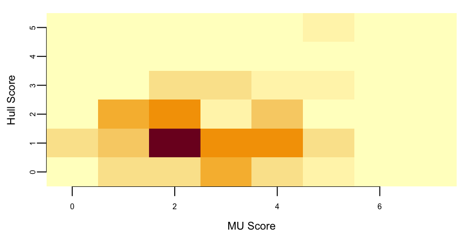

Figure 3.4: Simulation of MU vs Hull game.

Now we can calculate the number of times MU wins:

sum(x > y)
## 67

A model is only as good as its predictions. Let’s see how well our model predicted the outcome of the MU vs Hull game. The actual outcome was 0-1 (MU at Hull). The model predicted that most likely MU would score 1-2 (16 games out of 100). In our simulation 0-1 was the third most probable outcome (8 games out of 100). Man U wins 67 games out of 100; we should bet when odds ratio is below 67 to 100.

3.5 Poisson-Gamma: Learning about an Intensity

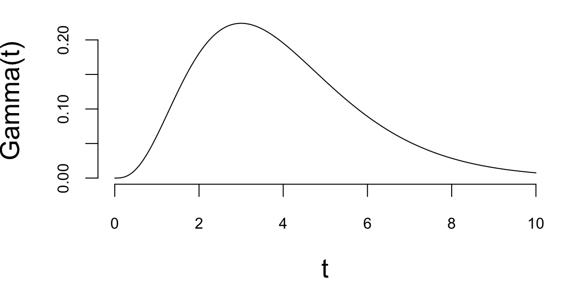
Consider a continuous-time stochastic process, $\left\{ N_{t}\right\} _{t\geq0}$, with $N_{0}=0$, counting the number of events that have occurred up to time $t$. The process is constant between event times, and jumps by one at event times: $\Delta N_{t}=N_{t}-N_{t-}=1,$ where $N_{t-}$ is the limit from the left. The probability of an event over the next short time interval, $\Delta t$ is $\lambda\Delta t$, and $N_{t}$ is called a Poisson process because \[ P\left[ N_{t}=k\right] =\frac{e^{-\lambda t}\left( \lambda t\right) ^{k}}{k!}\text{ for }k=1,\ldots \] which is the Poisson distribution; thus $N_{t}\sim Poi\left(\lambda t\right)$. A more general version of the Poisson process is a Cox process, or doubly stochastic point process.

Here, there is additional conditioning information in the form of state variables, $\left\{X_{t}\right\}_{t>0}$. The process now has two sources of randomness, one associated with the discontinuous jumps and another in the form of random state variables, $\left\{X_{t}\right\}_{t>0}$, that drive the intensity of the process. The intensity of the Cox process is $\lambda_{t}=\int_{0}^{t}\lambda\left( X_{s}\right) ds$, which is formally defined as \[ P\left[ N_{t}-N_{s}=k \mid \left\{ X_{u}\right\} _{s\leq u\leq t}\right] =\frac{\left( \int_{s}^{t}\lambda\left( X_{s}\right) ds\right) ^{k}\exp\left( -\int_{s}^{t}\lambda\left( X_{s}\right) ds\right)}{k!}, ~ \forall k \] Cox processes are very useful extensions to Poisson processes and are the basic building blocks of reduced form models of defaultable bonds.

The inference problem is to learn about $\lambda$ from a continuous-record of observations up to time $t$. The likelihood function is given by \[ p\left( N_{t}=k \mid \lambda\right) =\frac{\left( \lambda t\right) ^{k}% \exp\left( -\lambda t\right) }{k!}, \] and the MLE is $\widehat{\lambda}=N_{t}/t$. Notice that the total count $N_t$ and elapsed time $t$ together form the sufficient statistic for $\lambda$, since the likelihood depends on the data only through these two quantities. The MLE has the unattractive property that prior to the first event $\left\{ t:N_{t}=0\right\}$, the MLE is 0, despite the fact that the model explicitly assumes that events are possible. This problem often arises in credit risk contexts, where it would seem odd to assume that the probability of default is zero just because a default has not yet occurred.

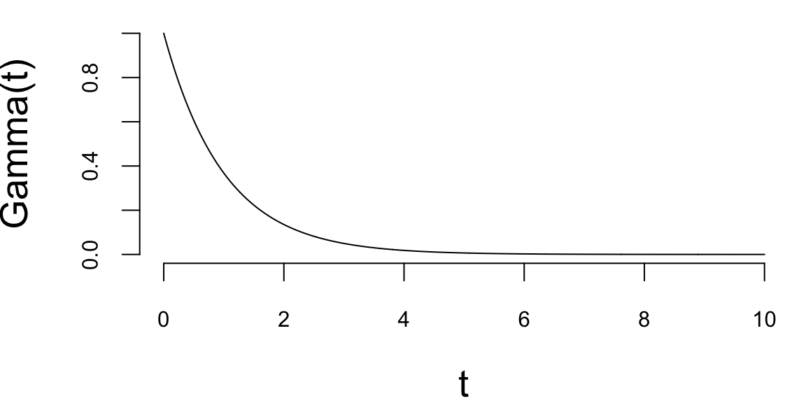
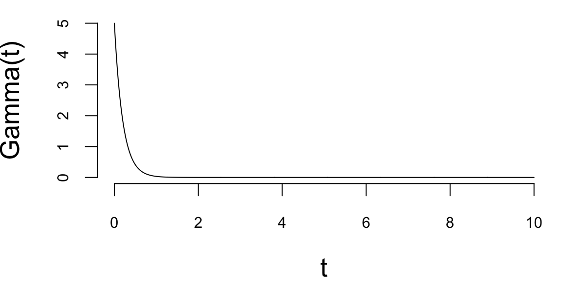
A natural prior for this model is the Gamma distribution, which has the following pdf \[ p\left( \lambda \mid a,A\right) =\frac{A^{a}}{\Gamma(a) }\lambda^{a-1}\exp\left( -A\lambda\right) \text{.} \tag{3.2}\] Like the beta distribution, a Gamma prior distribution allows for a variety of prior shapes and is parameterized by two hyperparameters. Combining the prior and likelihood, the posterior is also Gamma: \[ p\left( \lambda \mid N_{t}\right) \propto\frac{\left( \lambda\right) ^{N_{t}+a-1}\exp\left( -\lambda\left( t+A\right) \right) }{N_{t}!}% \sim\mathcal{G}\left( a_{t},A_{t}\right) , \] where $a_{t}=N_{t}+a$ and $A_{t}=t+A$. The expected intensity, based on information up to time $t$, is \[ \E{\lambda \mid N_{t}} =\frac{a_{t}}{A_{t}}=\frac{N_{t}% +a}{t+A}=w_{t}\frac{N_{t}}{t}+\left( 1-w_{t}\right) \frac{a}{A}, \] where the second line expresses the posterior mean in shrinkage form as a weighted average of the MLE and the prior mean, where $w_{t}=t/(t+A)$. In large samples, $w_{t}\rightarrow1$ and $\E{\lambda \mid N_{t}} \approx N_{t}/t=\widehat{\lambda}$.

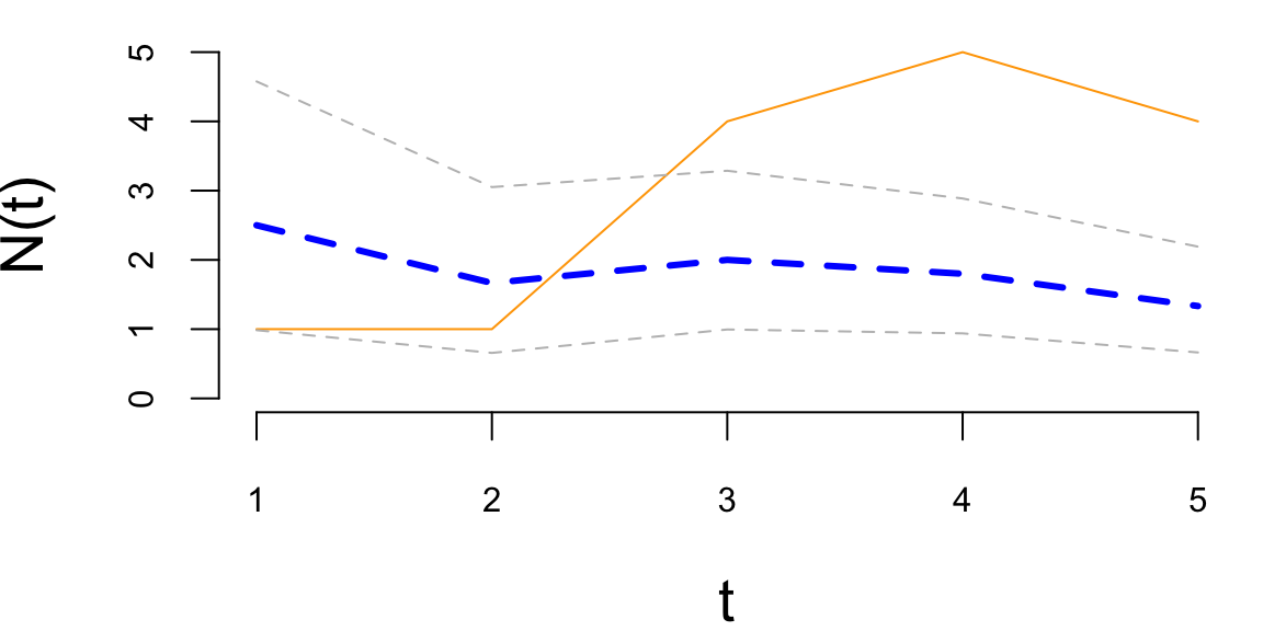
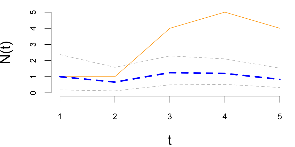
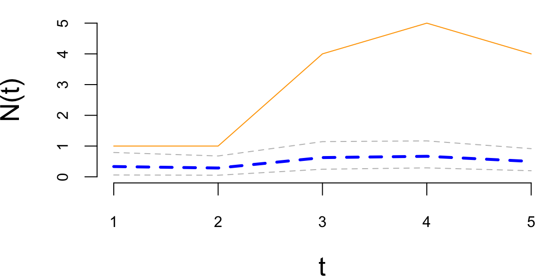
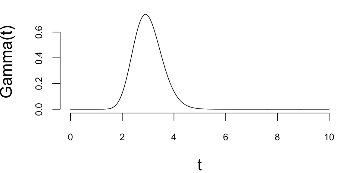
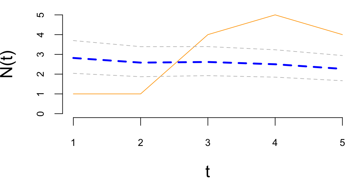
To understand the updating mechanics, Figure 3.5 (right column) displays a simulated sample path, posterior means, and (5%,95%) posterior quantiles for various prior configurations. In this case, time is measured in years, and the intensity used to simulate the data is $\lambda=1$, implying on average one event per year. The four prior configurations embody different beliefs. In the first case, in the middle left panel, $a=4$ and $A=1$ capture a high-activity prior that posits that jumps occur, on average, four times per year, and there is substantial prior uncertainty over the arrival rate, as the (5%,95%) prior quantiles are (1.37,7.75). In the second case, it captures a prior that is centered over the true value with modest prior uncertainty. The third case captures a low-activity prior, with a prior mean of 0.2 jumps/year. The fourth case captures a dogmatic prior that posits that jumps occur three times per year, with high confidence in these beliefs.

The priors were chosen to highlight different potential paths for Bayesian learning. The first thing to note from the priors is the discontinuity upward at event times, and the exponential decrease during periods of no events, both of which are generic properties of Bayesian learning in this model. If one thinks of the events as rare, this implies rapid revisions in beliefs at event times and a constant drop in estimates of the intensity in periods of no events. For the high-activity prior and the sample path observed, the posterior begins well above $\lambda=1$, and slowly decreases, getting close to $\lambda=1$ at the end of the sample. This can be somewhat contrasted with the low-activity prior, which has drastic revisions upward at jump times. In the dogmatic case, there is little updating at event times. The prior parameters control how rapidly beliefs change, with noticeable differences across the priors.

In all cases, the orange line shows the cumulative event count $N_t$, the blue dashed line represents the posterior mean of $\lambda$, and the grey dashed lines indicate the 5% and 95% posterior quantiles. The discontinuous upward jumps at event times and exponential decay during quiet periods are characteristic features of Bayesian learning in Poisson processes.

(a) High-activity: a = 4, A = 1; 4 events/year, Substantial prior uncertainty

Poisson event models are often embedded as portion of more complicated model to capture rare events such as stock market crashes, volatility surges, currency revaluations, or defaults. In these cases, prior distributions are often important–even essential–since it is common to build models with events that could, but have not yet occurred. These events are often called ‘Peso’ events. For example, in the case of modeling corporate defaults, a researcher wants to allow for a jump to default. This requires positing a prior distribution that places non-zero probability on an event occurring. Classical statistical methods have difficulties dealing with these situations since the MLE of the jump probability is zero until the first event occurs.

3.6 Exponential-Gamma Model

The Exponential distribution is often used to model waiting times between events, such as the time between independent arrivals in a Poisson process. The probability density function (PDF) is defined as: \[ p(x \mid \lambda) = \lambda e^{-\lambda x}, \quad x \geq 0 \] where $\lambda > 0$ is the rate parameter (inverse of the mean).

The Exponential-Gamma model assumes that the data follow an exponential distribution, and the rate parameter $\lambda$ follows a Gamma prior distribution. \[\begin{align*} \lambda &\sim \text{Gamma}(\alpha, \beta) \\ y_i \mid \lambda &\sim \text{Exponential}(\lambda) \end{align*}\]

The probability density function of the Gamma prior is: \[ p(\lambda \mid \alpha, \beta) = \frac{\beta^\alpha}{\Gamma(\alpha)} \lambda^{\alpha-1} e^{-\beta\lambda} \]

Given $n$ observations $y = (y_1, \ldots, y_n)$, the likelihood depends on the data only through the count $n$ and the sum $\sum_{i=1}^n y_i$, which form the sufficient statistics for $\lambda$. The posterior distribution of $\lambda$ is: \[ p(\lambda\mid y) \propto p(y \mid \lambda) p(\lambda) \propto \left( \prod_{i=1}^n \lambda e^{-\lambda y_i} \right) \lambda^{\alpha - 1} e^{-\beta\lambda} = \lambda^{\alpha + n - 1} e^{-(\beta + \sum y_i)\lambda} \] This is a Gamma distribution with updated parameters: \[ \lambda \mid y \sim \text{Gamma}\left(\alpha + n, \beta + \sum_{i=1}^n y_i\right). \] The posterior mean is: \[ \E{\lambda \mid y} = \frac{\alpha + n}{\beta + \sum y_i}. \]

This model is widely used in reliability engineering (failure rates) and survival analysis, where the rate of events is uncertain and varies across populations.

The Normal or Gaussian distribution is central to probability and statistical inference. Suppose that we are trying to predict tomorrow’s return on the S&P500. There’s a number of questions that come to mind

What is the random variable of interest?
How can we describe our uncertainty about tomorrow’s outcome?
Instead of listing all possible values we’ll work with intervals instead. The probability of an interval is defined by the area under the probability density function.

Returns are continuous (as opposed to discrete) random variables. Hence a normal distribution would be appropriate - but on what scale? We will see that on the log-scale a Normal distribution provides a good approximation.

The most widely used model for a continuous random variable is the normal distribution. Standard normal random variable $Z$ has the following properties

The standard Normal has mean $0$ and has a variance $1$, and is written as \[ Z \sim N(0,1) \] Then, we have the probability statements of interest \[\begin{align*} P(-1 <Z< 1) &=0.68\\ P(-1.96 <Z< 1.96) &=0.95\\ \end{align*}\] In R, we can find probabilities pnorm(1.96): 0.9750021 and quantiles qnorm(0.9750): 1.959964. The quantile function qnorm is the inverse of pnorm.

A random variable that follows normal distribution with general mean and variance $X \sim \mbox{N}(\mu, \sigma^2)$, has the following properties \[\begin{align*} p(\mu - 2.58 \sigma < X < \mu + 2.58 \sigma) &=0.99 \\ p(\mu - 1.96 \sigma < X < \mu + 1.96 \sigma) &=0.95 \, . \end{align*}\] The chance that $X$ will be within $2.58 \sigma$ of its mean is $99\%$, and the chance that it will be within $2\sigma$ of its mean is about $95\%$.

The probability model is written $X \sim N(\mu,\sigma^2)$, where $\mu$ is the mean and $\sigma^2$ is the variance. This can be transformed to a standardized normal via \[ Z =\frac{X-\mu}{\sigma} \sim N(0,1). \] For a Normal distribution, we know that $X \in [\mu-1.96\sigma,\mu+1.96\sigma]$ with probability 95%. This is a specific property of the Normal curve (the “Empirical Rule”). For any distribution, regardless of shape, we can use Chebyshev’s Inequality to bound the probability mass. It states that at least $100(1-1/k^2)$% of values lie within $k$ standard deviations of the mean:

At least 75% probability lies within $2\sigma$ ($k=2$).
At least 89% probability lies within $3\sigma$ ($k=3$).
At least $100(1-1/m^2)$% lies within $m\times \sigma$ of the mean $\mu$.

While the Normal distribution guarantees 95% within $2\sigma$, Chebyshev guarantees only 75%, reflecting the uncertainty given a lack of distributional assumptions.

Example 3.5 (Google Stock 2019) Consider observations of daily log-returns of a Google stock for 2019 Daily log-return on day $t$ is calculated by taking a logarithm of the ratio of the price at close of day $t$ and at close of day $t-1$ \[ y_t = \log\left(\dfrac{P_t}{P_{t-1}}\right) \] For example on January 3 of 2017, the open price is 778.81 and the close price was 786.140; then the log-return is $\log(786.140/778.81) = 0.0094$. It was empirically observed that log-returns follow a Normal distribution. This observation is a basis for Black-Scholes model with is used to evaluate future returns of a stock.

p <- read.csv("../data/GOOG2019.csv")$Adj.Close
n <- length(p)
r <- log(p[2:n] / p[1:(n - 1)])
hist(r, breaks = 30, col = "lightblue", main = "")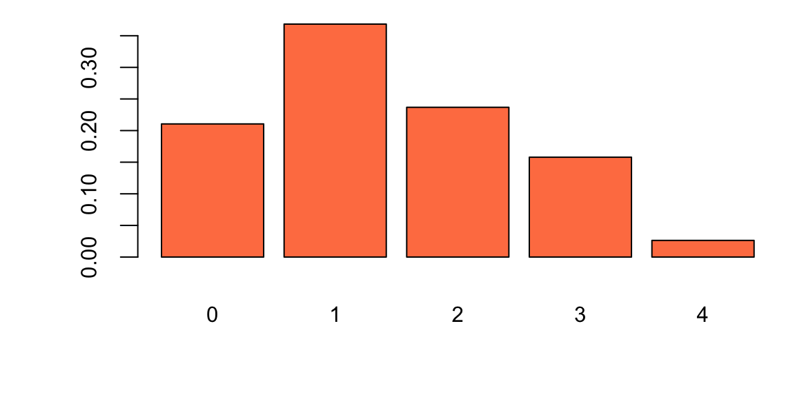

Observations on the far right correspond to the days when positive news was released, and on the far left correspond to bad news. Typically, those are days when the quarterly earnings reports are released.

To estimate the expected value $\mu$ (return) and standard deviation $\sigma$ (a measure of risk), we simply calculate their sample counterparts \[ \bar{x} = \frac{1}{n} \sum_{i=1}^n x_i, ~\mathrm{ and }~ s^2 = \frac{1}{n-1} \sum_{i=1}^n (x_i - \bar{x} )^2 \] The empirical (or sample) values $\bar x$ and $s^2$ are called the sample mean and sample variance. Here simply view them as our best guess about the mean and variance of the normal distribution model; then our probabilistic model for the next day’s return is then given by \[ R \sim N(\bar x, s^2). \]

Say we are interested in investing into Google and would like to calculated the expected return of our investment as well as the risk associated with this investment. We assume that the behavior of the returns in the future will be the same as in 2019.

n <- length(r)
rbar <- sum(r) / n
print(rbar)
## 0.00098
s2 <- sum((r - rbar)^2) / (n - 1)
print(s2)
## 0.00023
x <- seq(-0.08, 0.08, length.out = 200)
hist(r, breaks = 30, col = "lightblue", freq = F, main = "", xlab = "")
lines(x, dnorm(x, rbar, sqrt(s2)), col = "red", lwd = 3)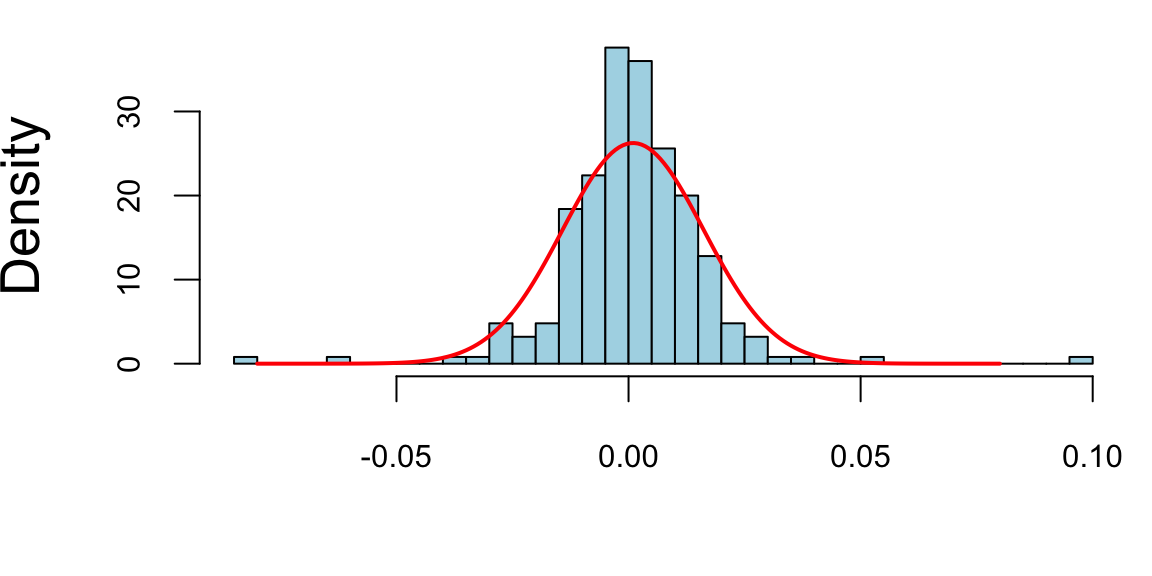

Histogram (blue) and fitted normal curve (red) of for the Google stock daily return data.

Now, assume I invest all my portfolio into Google. I can predict my annual return to be $251 \times 0.0009798$ = 0.2459348, and the risk (volatility) of my investment is $\sqrt{s^2}$ = 1.5198424% a year.

I can predict the risk of losing 3% or more in one day using my model is 1.93%.

pnorm(log(1 - 0.03), rbar, sqrt(s2)) * 100
## 1.9

mean(spret)
## 0.012
sd(spret)
## 0.043

3.7 Normal with Unknown Mean

Let $Y$ be a random variable with a normal distribution, $Y \sim N(\mu, \sigma^2)$. The mean $\mu$ is unknown, but the variance $\sigma^2$ is known. The likelihood function is given by \[ p(y \mid \mu) = \frac{1}{\sqrt{2\pi\sigma^2}}\exp\left(-\frac{1}{2\sigma^2}(y-\mu)^2\right) \] The MLE of $\mu$ is $\hat{\mu} = \bar{y}$, the sample mean. Normal prior for the mean parameter $\mu$ is conjugate to the normal likelihood. \[ \mu \sim N(\mu_0, \sigma_0^2) \] The posterior distribution is also normal. \[ p(\mu \mid y) \sim N(\mu_n, \sigma_n^2) \]

where \[ \mu_n = \frac{\sigma^2}{n\sigma_0^2 + \sigma^2}\mu_0 + \frac{n\sigma_0^2}{n\sigma_0^2 + \sigma^2}\bar{y} \] and \[ \sigma_n^2 = \frac{\sigma^2\sigma_0^2}{n\sigma_0^2 + \sigma^2} \] The posterior mean is a weighted average of the prior mean and the sample mean, with the weights being proportional to the precision of the prior and the likelihood. The posterior variance is smaller than the prior variance, and the sample size $n$ appears in the denominator. The posterior mean is a shrinkage estimator of the sample mean, and the amount of shrinkage is controlled by the prior variance $\sigma_0^2$. A couple of observations \[ \frac{\sigma^2}{n\sigma_0^2 + \sigma^2} \rightarrow 0 \text{ and } \frac{n\sigma_0^2}{n\sigma_0^2 + \sigma^2}\rightarrow 1, \text{ as } n \rightarrow \infty. \] Further, \[ \frac{\sigma^2\sigma_0^2}{n\sigma_0^2 + \sigma^2} \rightarrow 0 \text{ as } n \rightarrow \infty. \]

Example 3.6 (Stylized Example) Assuming the prior distribution $\mu \sim N(-1,1)$, say we observed $y=2$, and we want to update our beliefs about $\mu$. The likelihood function is $p(y \mid \mu) = N(\mu,2^2)$, and the posterior distribution is \[ p(\mu \mid y) \propto p(y \mid \mu) p(\mu) = N(y\mid \mu,2^2) N(\mu\mid -1,1) = N(-0.4,0.894^2). \]

## "Posterior mean: -0.400000, Posterior standard deviation: 0.894427"

Graphically we can represent this as follows

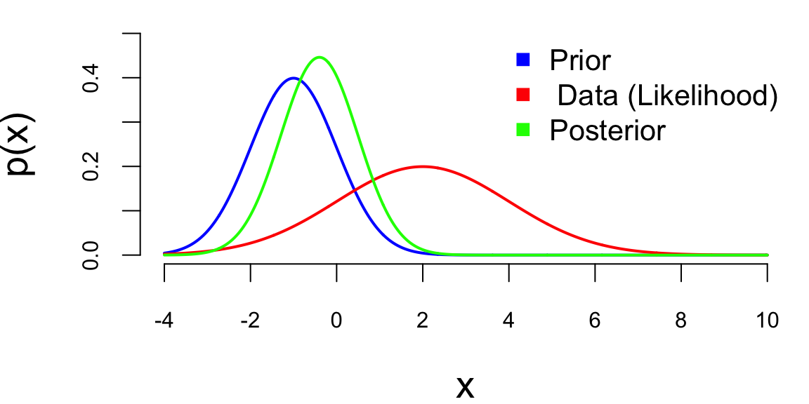
Note: the posterior mean is between those of prior and likelihood and posterior variance is lower than variance of both prior and likelihood; this is effect of combining information from data and prior!

More generally, when we observe $n$ independent and identically distributed (i.i.d.) data points $y_1,\ldots,y_n$ from a normal distribution with known variance $\sigma^2$, the likelihood function is given by \[ p(y \mid \mu) = N(\bar y\mid \mu,\sigma^2/n),~ \text{where}~ \bar y = \frac{1}{n}\sum_{i=1}^n y_i. \] Note that average over the observed data $\bar y = \mathrm{Ave}(y_1,\ldots,y_n)$ is the sufficient statistics for the mean $\mu$. The prior distribution is given by \[ p(\mu) = N(\mu\mid \mu_0,\sigma_0^2) \] The posterior distribution is given by \[ \begin{split} p(\mu\mid y) & \propto \exp\Bigg[{\frac{-\mu^2+2\mu\mu_0-\mu_0^2}{2\sigma_0^2}}\Bigg]\exp\Bigg[{\frac{-\mu^2+2\mu\bar{y}-\bar{y}^2}{2\sigma^2/n}}\Bigg] \\ & \propto \exp\Bigg[{\frac{-\mu^2+2\mu\mu_0}{2\sigma_0^2}}\Bigg]\exp\Bigg[{\frac{-\mu^2+2\mu\bar{y}}{2\sigma^2/n}}\Bigg]. \\ \end{split} \] Now we combine the terms \[ \begin{split} p(\mu\mid y) & \propto \exp\Bigg[{\frac{(-\mu^2+2\mu\mu_0)\sigma^2 +(-\mu^2+2\mu\bar{y})n\sigma_0^2}{2\sigma_0^2\sigma^2}}\Bigg]. \\ \end{split} \] Now re-arrange and combine $\mu^2$ and $\mu$ terms \[ \begin{split} p(\mu\mid y) & \propto \exp\Bigg[{\frac{-\mu^2(n\sigma_0^2+\sigma^2)+2\mu(\mu_0\sigma^2+ \bar{y}n\sigma_0^2) }{2\sigma_0^2\sigma^2}}\Bigg] \\ & \propto \exp\Bigg[{\frac{-\mu^2+2\mu\left(\frac{\mu_0\sigma^2 + \bar{y}n\sigma_0^2}{n\sigma_0^2+\sigma^2}\right) }{2(\sigma_0^2\sigma^2) /(n\sigma_0^2+\sigma^2)}}\Bigg]. \\ \end{split} \] Now we add constants which do not depend upon $\mu$ to complete the square in the numerator: \[ \begin{split} p(\mu\mid y) & \propto \exp\Bigg[{\frac{-\bigg(\mu - \frac{\mu_0\sigma^2 + \bar{y}n\sigma_0^2}{n\sigma_0^2+\sigma^2}\bigg)^2 }{2(\sigma_0^2\sigma^2) /(n\sigma_0^2+\sigma^2)}}\Bigg]. \\ \end{split} \] Finally we get the posterior mean \[ \mu_n = \frac{\mu_0\sigma^2+ \bar{y}n\sigma_0^2}{n\sigma_0^2+\sigma^2} = \mu_0\frac{\sigma^2}{n\sigma_0^2+\sigma^2} + \bar{y}\frac{n\sigma_0^2}{n\sigma_0^2+\sigma^2} \] and the posterior variance \[ \sigma_n^2 = \frac{\sigma_0^2\sigma^2}{n\sigma_0^2+\sigma^2}. \]

Example 3.7 (Chicago Bears 2014–2015 Season) The Chicago Bears are a professional American football team based in Chicago, Illinois. The Bears were a young team in 2014–2015 and were last in their division. This season the Chicago Bears suffered back-to-back $50$-points defeats and lost to Patriots and Packers.

Patriots-Bears $51-23$
Packers-Bears $55-14$

Their next game was at home against the Minnesota Vikings. Current line against the Vikings was $-3.5$ points. Slightly over a field goal. What’s the Bayes approach to learning the line? We use hierarchical data and Bayes learning to update our beliefs in light of new information. The current average win/lose this year can be modeled as a normal distribution with mean $\mu$ and standard deviation $\sigma$. We assume that $\mu$ is normally distributed with mean $\mu_0$ and standard deviation $\tau$. \[\begin{align*} \bar{y} \mid \mu & \sim N \left ( \mu , \frac{\sigma^2}{n} \right ) \sim N \left ( \mu , \frac{18.34^2}{9} \right )\\ \mu & \sim N( 0 , \tau^2 ) \end{align*}\] Here $n =9$ games so far. With $s = 18.34$ points. We assume the pre-season prior mean $\mu_0 = 0$, standard deviation $\tau = 4$. Base on the observed data so-far: $\bar{y} = -9.22$.

The Bayes Shrinkage estimator is then \[ \E{\mu \mid \tau, \bar y} = \frac{ \tau^2 }{ \tau^2 + \frac{\sigma^2}{n} }\bar{y} . \]

The shrinkage factor is $0.3$! That’s quite a bit of shrinkage. Why? Our updated estimator is \[ \E{\mu \mid \bar{y}, \tau} = -2.76 > -3.5 \] where current line is $-3.5$.

Based on our hierarchical model, this is an over-reaction. One point change on the line is about $3$% on a probability scale.
Alternatively, calculate a market-based $\tau$ given line $=-3.5$. \[ w = \frac{3.5}{9.22} = 0.38, \quad \tau^2 = \frac{w}{1-w}\,\frac{\sigma^2}{n} \approx 22.9. \]
The market-based $\tau$ is $\approx 4.8$ points.

bears <- c(-3, 8, 8, -21, -7, 14, -13, -28, -41)
print(mean(bears))
## -9.2
print(sd(bears))
## 18
tau <- 4
sig2 <- sd(bears) * sd(bears) / 9
print(tau^2 / (sig2 + tau^2))
## 0.3
print(0.29997 * -9.22)
## -2.8
print(pnorm(-2.76 / 18))
## 0.44

Home advantage is worth $3$ points. The actual result of the game is Bears 21, Vikings 13.

Posterior Predictive

After estimating the parameters, using the posterior distribution, we often want to predict future observations. This is done using the posterior predictive distribution. The posterior predictive distribution is the distribution of a new observation $y_{n+1}$ given the observed data $y_1,\ldots,y_n$. The posterior predictive distribution is given by

\[\begin{align*} p(y_{n+1} \mid & y_1,\ldots,y_n) = \int p(y_{n+1} \mid \mu) p(\mu \mid y_1,\ldots,y_n) d\mu \\ & = \int N(y_{n+1} \mid \mu, \sigma^2) N(\mu \mid \mu_n, \sigma_n^2) d\mu = N(y_{n+1} \mid \mu_n, \sigma_n^2 + \sigma^2). \end{align*}\] This follows from the general properties of the Gaussian distribution

3.8 Normal with Unknown Variance

Consider another example, when mean $\mu$ is fixed, and variance is a random variable which follows some distribution $\sigma^2 \sim p(\sigma^2)$. Given an observed sample $y$, we can update the distribution over variance using Bayes’ rule \[ p(\sigma^2 \mid y) = \dfrac{p(y\mid \sigma^2 )p(\sigma^2)}{p(y)}. \] Now, the total probability in the denominator can be calculated as \[ p(y) = \int p(y\mid \sigma^2 )p(\sigma^2) d\sigma^2. \]

A conjugate prior that leads to analytically calculable integral for variance under the normal likelihood is the inverse Gamma. When the mean $\mu$ is known, the sufficient statistic for $\sigma^2$ is the sum of squared deviations $\sum_{i=1}^n(y_i - \mu)^2$. Thus, if \[ \sigma^2 \mid \alpha,\beta \sim IG(\alpha,\beta) = \dfrac{\beta^{\alpha}}{\Gamma(\alpha)}\sigma^{2(-\alpha-1)}\exp\left(-\dfrac{\beta}{\sigma^2}\right) \] and \[ y \mid \mu,\sigma^2 \sim N(\mu,\sigma^2) \] Then the posterior distribution is another inverse Gamma $IG(\alpha_{\mathrm{posterior}},\beta_{\mathrm{posterior}})$, with \[ \alpha_{\mathrm{posterior}} = \alpha + \dfrac{1}{2}, ~~\beta_{\mathrm{posterior}} = \beta + \dfrac{(y-\mu)^2}{2}. \]

Now, the predictive distribution over $y$ can be calculated by \[ p(y_{new}\mid y) = \int p(y_{new},\sigma^2\mid y)p(\sigma^2\mid y)d\sigma^2. \] Which happens to be a $t$-distribution with $2\alpha_{\mathrm{posterior}}$ degrees of freedom, mean $\mu$ and variance $\beta_{\mathrm{posterior}}/(\alpha_{\mathrm{posterior}}-1)$.

The Normal-Gamma Model

Now, consider the case when both mean and variance are unknown. To simplify the formulas, we work with precision $\tau = 1/\sigma^2$. The Normal-Gamma distribution is a conjugate prior for a Normal likelihood with unknown mean and precision. Given data $y = \{y_1,\ldots,y_n\}$, we assume: \[ y_i \mid \theta, \tau \sim N(\theta, 1/\tau) \]

For this model, the sufficient statistics are the sample mean $\bar{y} = n^{-1}\sum_{i=1}^n y_i$, the sample size $n$, and the sum of squared deviations $\sum_{i=1}^n(y_i - \bar{y})^2$. The Normal-Gamma prior distribution is defined as: \[ \theta\mid \mu,\tau,\nu \sim N(\mu, 1/(\tau \nu)), \quad \tau \mid \alpha, \beta \sim \text{Gamma}(\alpha, \beta). \] Conditional on precision $\tau$, the mean $\theta$ is Normal with precision $\nu\tau$. The marginal distribution of $\tau$ is Gamma. Note that $\theta$ and $\tau$ are not independent in the joint prior.

Given the likelihood: \[ p(y\mid \theta, \tau) \propto \tau^{n/2}\exp\left(-\frac{\tau}{2}\sum_{i=1}^n(y_i-\theta)^2\right) \] and the prior, the posterior distribution is also Normal-Gamma with parameters: \[ \begin{aligned} \mu_n &= \dfrac{\nu\mu + n\bar{y}}{\nu+n},\\ \nu_n &= \nu+n,\\ \alpha_n &= \alpha + \dfrac{n}{2},\\ \beta_n &= \beta + \dfrac{1}{2}\sum_{i=1}^n(y_i-\bar{y})^2 + \dfrac{n\nu}{2(\nu+n)}(\bar{y}-\mu)^2. \end{aligned} \] where $\bar{y} = n^{-1}\sum_{i=1}^n y_i$ is the sample mean and $n$ is the sample size. The posterior distribution is a normal-Gamma distribution with parameters $\mu_n, \nu_n, \alpha_n, \beta_n$.

Credible Intervals for Normal-Gamma Model Posterior Parameters

The precision posterior follows a Gamma distribution with parameters $\alpha_n, \beta_n$, thus we can use quantiles of the Gamma distribution to calculate credible intervals. A symmetric $100(1-c)%$ credible interval $[g_{c/2},g_{1-c/2}]$ is given by $c/2$ and $1-c/2$ quantiles of the gamma distribution. To find credible interval for the variance $v = 1/\tau$, we simply use \[ [1/g_{1-c/2},1/g_{c/2}]. \] and for standard deviation $s = \sqrt{v}$ we use \[ [\sqrt{1/g_{1-c/2}},\sqrt{1/g_{c/2}}]. \] To find credible interval over the mean $\theta$, we need to integrate out the precision $\tau^{-2}$ from the posterior distribution. The marginal distribution of $\theta$ is a Student’s $t$-distribution with parameters center at $\mu_n$, variance $\beta_n/(\nu_n\alpha_n)$, and degrees of freedom $2\alpha_n$.

3.9 Multivariate Normal

We write $X \sim N(\mu,\Sigma)$ for a $d$-dimensional multivariate normal random vector with mean vector $\mu \in \mathbb{R}^d$ and covariance matrix $\Sigma \in \mathbb{R}^{d\times d}$, where $\Sigma$ is symmetric and positive definite. If the linear algebra below is unfamiliar (transpose, inverse, determinant, positive definiteness), see Appendix A. Its density is \[ p(x\mid \mu,\Sigma) = \frac{1}{(2\pi)^{d/2}|\Sigma|^{1/2}}\exp\left(-\frac{1}{2}(x-\mu)^\top \Sigma^{-1}(x-\mu)\right), \qquad x\in\mathbb{R}^d. \] The multivariate normal is the workhorse distribution for joint modeling, conditioning, and linear transformations.

In the multivariate case, the normal-normal model is \[ \theta \sim N(\mu_0,\Sigma_0), \quad y \mid \theta \sim N(\theta,\Sigma). \] For a single multivariate observation, $y$ itself serves as the sufficient statistic for $\theta$. More generally, for $n$ independent observations $y_1,\ldots,y_n$, the sample mean $\bar{y} = n^{-1}\sum_{i=1}^n y_i$ is the sufficient statistic. The posterior distribution is \[ \theta \mid y \sim N(\mu_1,\Sigma_1), \] where \[ \Sigma_1 = (\Sigma_0^{-1} + \Sigma^{-1})^{-1}, \quad \mu_1 = \Sigma_1(\Sigma_0^{-1}\mu_0 + \Sigma^{-1}y). \] The predictive distribution is \[ y_{new} \mid y \sim N(\mu_1,\Sigma_1 + \Sigma). \]

Example 3.8 (Satya Nadella: CEO of Microsoft) In 2014, Satya Nadella became the CEO of Microsoft. The stock price of Microsoft has been on a steady rise since then. Suppose that you are a portfolio manager and you are interested in analyzing the returns of Microsoft stock compared to the market.

Suppose you are managing a portfolio with two positions stock of Microsoft (MSFT) and an index fund that follows S&P500 index and tracks overall market performance. We are interested in estimating the mean returns of the positions in our portfolio. You believe that the returns are normally distributed and are related to each other. You have prior beliefs about these returns, which are also normally distributed. We will use what is called the empirical prior for the mean returns. This is a prior that is based on historical data. The empirical prior is a good choice when you have a lot of historical data and you believe that the future mean returns will be similar to the historical mean returns. We assume the prior for the mean returns is a bivariate normal distribution; let $\mu_0 = (\mu_{M}, \mu_{S})$ represent the prior mean returns for the stocks. The covariance matrix $\Sigma_0$ captures your beliefs about the variability and the relationship between these stocks’ returns in the prior. We will use the sample mean and covariance matrix of the historical returns as the prior mean and covariance matrix. The prior covariance matrix is given by \[ \Sigma_0 = \begin{bmatrix} \sigma_{M}^2 & \sigma_{MS} \\ \sigma_{MS} & \sigma_{S}^2 \end{bmatrix}, \] where $\sigma_{M}^2$ and $\sigma_{S}^2$ are the sample variances of the historical returns of MSFT and SPY, respectively, and $\sigma_{MS}$ is the sample covariance of the historical returns of MSFT and SPY. The prior mean is given by \[ \mu_0 = \begin{bmatrix} \mu_{M} \\ \mu_{S} \end{bmatrix}, \] where $\mu_{M}$ and $\mu_{S}$ are the sample means of the historical returns of MSFT and SPY, respectively. The likelihood of observing the data, given the mean returns, is also a bivariate normal distribution. The mean of this distribution is the true (but unknown) mean returns $\mu = [\mu_A, \mu_B]$. The covariance matrix $\Sigma$ of the likelihood represents the uncertainty in your data. We will use the sample mean and covariance matrix of the observed returns as the likelihood mean and covariance matrix. The likelihood covariance matrix is given by \[ \Sigma = \begin{bmatrix} \sigma_{M}^2 & \sigma_{MS} \\ \sigma_{MS} & \sigma_{S}^2 \end{bmatrix}, \] where $\sigma_{M}^2$ and $\sigma_{S}^2$ are the sample variances of the observed returns of MSFT and SPY, respectively, and $\sigma_{MS}$ is the sample covariance of the observed returns of MSFT and SPY. The likelihood mean is given by \[ \mu = \begin{bmatrix} \mu_{M} \\ \mu_{S} \end{bmatrix}, \] where $\mu_{M}$ and $\mu_{S}$ are the sample means of the observed returns of MSFT and SPY, respectively. In a Bayesian framework, you update your beliefs (prior) about the mean returns using the observed data (likelihood). The posterior distribution, which combines your prior beliefs and the new information from the data, is also a bivariate normal distribution. The mean $\mu_{\text{post}}$ and covariance $\Sigma_{\text{post}}$ of the posterior are calculated using Bayesian updating formulas, which involve $\mu_0$, $\Sigma_0$, $\mu$, and $\Sigma$. Because both the prior and the likelihood describe a sample mean of many daily returns rather than a single return, each covariance is scaled by its number of observations ($\Sigma_0/n_{\text{prior}}$ and $\Sigma/n_{\text{obs}}$), so that the data precision grows with the sample size.

We use observed returns prior to Nadella’s becoming CEO as our prior and analyze the returns post 2014. Thus, our observed data include the July 2015–Dec 2023 period. We assume the likelihood of observing these data, given the mean returns, is also a bivariate normal distribution. The mean of this distribution is the true (but unknown) mean returns. The covariance matrix $Sigma$ of the likelihood represents the uncertainty in your data and is calculated from the overall observed returns data from 2001 to 2023.

getSymbols(c("MSFT", "SPY"), from = "2001-01-01", to = "2023-12-31")
s <- 3666 # 2015-07-30
prior <- 1:s
obs <- s:nrow(MSFT) # post covid
# obs = 5476:nrow(MSFT) # 2022-10-06 bull run if 22-23
a <- as.numeric(dailyReturn(MSFT))
c <- as.numeric(dailyReturn(SPY))
# Prior on the mean return: prior-period covariance scaled to the sample mean
n_prior <- length(prior)
mu0 <- c(mean(a[prior]), mean(c[prior]))
Sigma0 <- cov(data.frame(a = a[prior], c = c[prior])) / n_prior
# Data: the sample mean of n_obs returns has covariance Sigma / n_obs
n_obs <- length(obs)
mu <- c(mean(a[obs]), mean(c[obs]))
Sigma <- cov(data.frame(a = a, c = c)) / n_obs
# Posterior
SigmaPost <- solve(solve(Sigma0) + solve(Sigma))
muPost <- SigmaPost %*% (solve(Sigma0) %*% mu0 + solve(Sigma) %*% mu)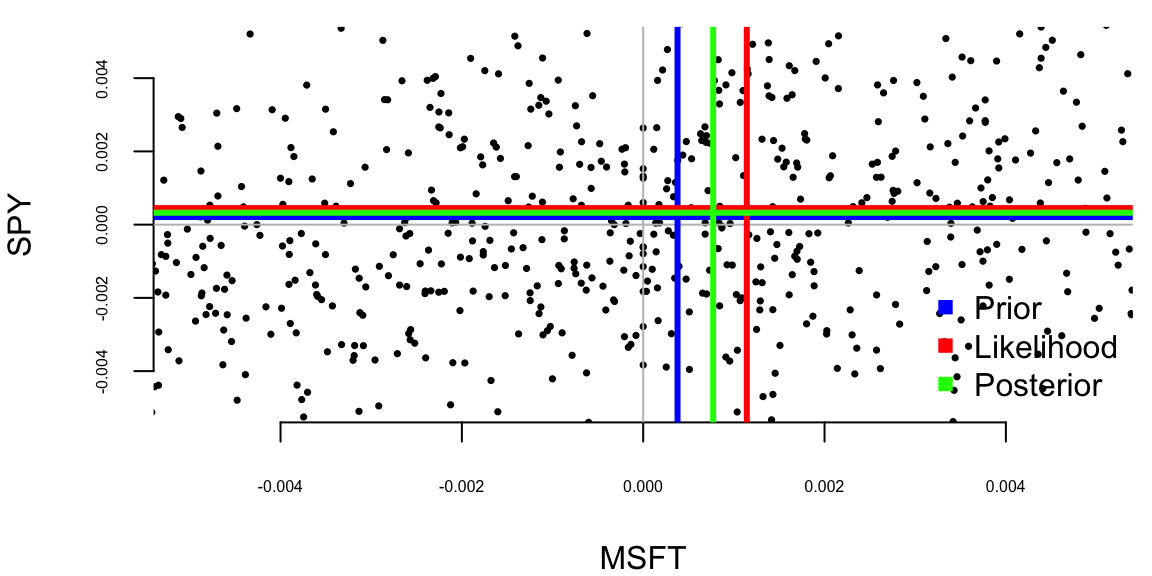

Figure 3.7: Plotting Portfolio Updating with MSFT and SPY.

We can see the posterior mean for SPY is close to the prior mean, while the posterior mean for MSFT is further away. The performance of MSFT was significantly better past 2015 compared to SPY. The posterior mean (green) represents mean reversion value. We can think of it a expected mean return if the performance of MSFT starts reverting to its historical averages.

This model is particularly powerful because it can be extended to more dimensions (more stocks) and can include more complex relationships between the variables. It’s often used in finance, econometrics, and other fields where understanding the joint behavior of multiple normally-distributed variables is important.

3.10 Mixtures of Conjugate Priors

A mixture of conjugate priors combines multiple conjugate components with weights $\pi_k$, creating a more flexible prior when no single conjugate family fits the problem. It is most useful when the data are generated from a mixture of distributions, each component arising from a different subpopulation.

If $p_1(x),\ldots,p_k(x)$ are proper density functions and $\pi_1,\ldots,\pi_k$ are non-negative weights that sum to 1, then the mixture distribution is given by \[ p(x) = \sum_{i=1}^k \pi_i p_i(x). \] It is easy to show that $p(x)$ is a proper density. Indeed, given domain $x\in A\subset \mathbb{R}$ we have \[ \int_A p(x)dx = \sum_{i=1}^k \pi_i \int_A p_i(x)dx = \sum_{i=1}^k \pi_i = 1. \]

Assume our prior is a mixture of distributions, that is \[ \theta \sim p(\theta) = \sum_{k=1}^K \pi_k p_k(\theta). \] Then the posterior is also a mixture of normal distributions, that is \[ p(\theta\mid y) = p(y\mid \theta)\sum_{k=1}^K \pi_k p_k(\theta)/Z. \] We introduce a normalizing constant for each component \[ Z_k = \int p(y\mid \theta)p_k(\theta)d\theta. \] then \[ p_k(\theta\mid y) = p_k(\theta)p(y\mid \theta)/Z_k \] is a proper distribution and our posterior is a mixture of these distributions \[ p(\theta\mid y) = \sum_{k=1}^K \pi_k Z_k p_k(\theta\mid y)/Z. \] Meaning that we need to require \[ \dfrac{\sum_{k=1}^K \pi_k Z_k}{Z} = 1, \quad \text{or} \quad Z = \sum_{k=1}^K \pi_k Z_k. \] Then the posterior density is a mixture \[ p(\theta\mid y) = \sum_{k=1}^K \hat \pi_k p_k(\theta \mid y). \]

Consider an example of a mixture of two normal distributions. The prior distribution is a mixture of two normal distributions, that is \[ \mu \sim 0.5 N(0,1) + 0.5 N(5,1). \] The likelihood is a normal distribution with mean $\mu$ and variance 1, that is \[ y \mid \mu \sim N(\mu,1). \] The posterior distribution is a mixture of two normal distributions, that is \[ p(\mu \mid y) \propto \phi(y\mid \mu,1) \left(0.5 \phi(\mu\mid 0,1) + 0.5 \phi(\mu\mid 5,1)\right), \] where $\phi(x\mid \mu,\sigma^2)$ is the normal distribution with mean $\mu$ and variance $\sigma^2$. We can calculate it using a property of a normal distribution \[ \phi(x\mid \mu_1,\sigma_1^2)\phi(x\mid \mu_2,\sigma_2^2) = \phi(x\mid \mu_3,\sigma_3^2)\phi(\mu_1-\mu_2\mid 0,\sigma_1^2+\sigma_2^2) \] where \[ \mu_3 = \dfrac{\mu_1/\sigma_1^2 + \mu_2/\sigma_2^2}{1/\sigma_1^2 + 1/\sigma_2^2}, \quad \sigma_3^2 = \dfrac{1}{1/\sigma_1^2 + 1/\sigma_2^2}. \]

Given, we observed $y = 2$, we can calculate the posterior distribution for $\mu$

mu0 <- c(0, 5)
sigma02 <- c(1, 1)
w0 <- c(0.5, 0.5)
y <- 2
mu3 <- (mu0 / sigma02 + y) / (1 / sigma02 + 1)
sigma3 <- 1 / (1 / sigma02 + 1)
Z <- dnorm(y - mu0, 0, sqrt(1 + sigma02)) * w0
w <- Z / sum(Z)
# To add a new line in sprintf, use "\n" inside the format string.
print("Component parameters:")
## "Component parameters:"
sprintf(
  "Mean = (%1.1f,%2.1f)  Var = (%1.1f,%1.1f)  weights = (%1.2f,%1.2f)",
  mu3[1], mu3[2], sigma3[1], sigma3[2], w[1], w[2]
)
## "Mean = (1.0,3.5)  Var = (0.5,0.5)  weights = (0.78,0.22)"

Table 3.1 collects the densities, means, and variances of the random variables used most often in the chapters that follow.

Table 3.1: Summary table of commonly used random variables.

Name	$\theta$	PDF	Mean	Variance	Support
Normal	$\mu, \sigma^2$	$\frac{1}{\sqrt{2\pi\sigma^2}}\exp\left(-\frac{(x-\mu)^2}{2\sigma^2}\right)$	$\mu$	$\sigma^2$	$x \in \mathbb{R}$
Exponential	$\lambda$	$\lambda e^{-\lambda x}$	$\frac{1}{\lambda}$	$\frac{1}{\lambda^2}$	$x \geq 0$
Gamma	$\alpha, \beta$	$\frac{\beta^\alpha}{\Gamma(\alpha)}x^{\alpha-1}e^{-\beta x}$	$\frac{\alpha}{\beta}$	$\frac{\alpha}{\beta^2}$	$x \geq 0$
Poisson	$\lambda$	$\frac{e^{-\lambda}\lambda^x}{x!}$	$\lambda$	$\lambda$	$x \in \mathbb{N}$
Binomial	$n, p$	$\binom{n}{x}p^x(1-p)^{n-x}$	$np$	$np(1-p)$	$x \in \{0, 1, \ldots, n\}$
Bernoulli	$p$	$p^x(1-p)^{1-x}$	$p$	$p(1-p)$	$x \in \{0, 1\}$
Multinomial	$n, \boldsymbol{p}$	$\frac{n!}{x_1!x_2!\cdots x_k!}p_1^{x_1}p_2^{x_2}\cdots p_k^{x_k}$	$np_i$	$np_i(1-p_i)$	$\sum x_i = n, x_i \in \{0,1,\dots,n\}$
Beta	$\alpha, \beta$	$\frac{\Gamma(\alpha + \beta)}{\Gamma(\alpha)\Gamma(\beta)}x^{\alpha-1}(1-x)^{\beta-1}$	$\frac{\alpha}{\alpha + \beta}$	$\frac{\alpha\beta}{(\alpha + \beta)^2(\alpha + \beta + 1)}$	$x \in [0, 1]$
Inverse Gamma	$\alpha, \beta$	$\frac{\beta^\alpha}{\Gamma(\alpha)}x^{-\alpha-1}e^{-\frac{\beta}{x}}$	$\frac{\beta}{\alpha-1}$	$\frac{\beta^2}{(\alpha-1)^2(\alpha-2)}$	$x > 0$

Table 3.2 summarizes the conjugate prior distributions for common likelihoods. Thus far, we’ve considered the Normal-Normal model with both known and unknown variance as well as Poisson-Gamma and Beta Binomial. The other pairs are left as an exercise. Given observed data $x = (x_1,\ldots,x_n)$ and $s = \sum_{i=1}^nx_i$, $\bar x = s/n$. For each conjugate pair, the table lists the sufficient statistics that summarize all information in the data relevant to the parameter. The posterior depends on the data only through these sufficient statistics, which is a key property of conjugate families.

Table 3.2: Conjugate prior table for common likelihoods.

Likelihood	Prior	Prior Parameters	Model Parameters	Sufficient Statistics	Posterior Parameters
Normal (known $\sigma^2$)	Normal	$\mu_0, \sigma^2_0$	$\mu$	$\bar x, n$	$\frac{n\sigma^2_0 \bar x + \sigma^2 \mu_0}{\sigma^2 + n\sigma^2_0},~\frac{\sigma^2\sigma_0^2}{n\sigma_0^2+\sigma^2}$
Normal (known $\mu$)	Inverse Gamma	$\alpha,\beta$	$\sigma^2$	$\sum(x_i-\mu)^2, n$	$\alpha+n/2, \beta + \frac{1}{2}\sum(x_i-\mu)^2$
Binomial ($m$ trials)	Beta	$\alpha, \beta$	$p$	$s, n$	$\alpha + s, \beta + nm - s$
Poisson	Gamma	$\alpha, \beta$	$\lambda$	$s, n$	$\alpha + s, \beta + n$
Exponential	Gamma	$\alpha, \beta$	$\lambda$	$s, n$	$\alpha + n, \beta + s$
Multinomial	Dirichlet	$\alpha \in \mathbb{R}^k$	$p \in \mathbb{R}^k$	$s_j$ for each category $j$	$\alpha+s$
Normal	Normal-inverse gamma	$\mu_0, \nu, \alpha, \beta$	$\mu, \sigma$	$\bar x, \sum(x_i-\bar x)^2, n$	$\frac{\nu\mu_0+n\bar{x}}{\nu+n} ,\, \nu+n,\, \alpha+\frac{n}{2} ,\,$ $\beta + \tfrac{1}{2} \sum_{i=1}^n (x_i - \bar{x})^2 + \frac{n\nu}{\nu+n}\frac{(\bar{x}-\mu_0)^2}{2}$

These conjugate relationships simplify Bayesian calculations by ensuring that the posterior distributions are in the same family as the priors.

3.11 Bayesian Computation: When Conjugacy Breaks

Conjugate priors are powerful because they keep the posterior in a familiar family and allow analytic updating. But most realistic Bayesian models are not conjugate: likelihoods can be non-Gaussian, priors can encode structure (sparsity, hierarchy), and predictors can enter through nonlinear functions. In those settings, the posterior still exists, but we cannot usually write it down in closed form.

The default remedy is approximation by simulation. The unifying idea is simple: if we can draw samples $\theta^{(1)},\ldots,\theta^{(N)} \sim p(\theta\mid y)$, then posterior summaries become Monte Carlo averages. For example, for any function $g(\theta)$, \[ \E{g(\theta)\mid y} \approx \frac{1}{N}\sum_{n=1}^N g(\theta^{(n)}). \] This is the same law-of-large-numbers logic discussed in Chapter 1, but applied to posterior distributions rather than to a known data-generating distribution.

Posterior Consistency and the Law of Large Numbers

The law of large numbers provides theoretical justification for Bayesian learning. As we collect more data, the posterior distribution concentrates around the true parameter value, regardless of the prior. This phenomenon, known as posterior consistency, follows from the fact that the likelihood function—being a product of many terms—is dominated by the data for large samples.

Consider estimating the mean $\mu$ of a normal distribution from i.i.d. observations $x_1, \ldots, x_n \sim N(\mu, \sigma^2)$ with a prior $\mu \sim N(\mu_0, \tau_0^2)$. The posterior mean is:

\[ \E{\mu \mid x_1, \ldots, x_n} = \frac{\tau_0^{-2}\mu_0 + n\sigma^{-2}\bar{x}_n}{\tau_0^{-2} + n\sigma^{-2}} \]

As $n \to \infty$, the data term $n\sigma^{-2}\bar{x}_n$ dominates, and by the law of large numbers, $\bar{x}_n \to \mu$ almost surely. Thus:

\[ \E{\mu \mid x_1, \ldots, x_n} \to \mu \quad \text{almost surely}. \]

The posterior concentrates at $\mu$, regardless of the prior $\mu_0$. The prior matters for small samples but becomes negligible for large samples—a reassuring property that ensures different researchers with different priors eventually reach consensus as evidence accumulates.

Monte Carlo Methods

Monte Carlo simulation is also justified by the law of large numbers. To approximate an expectation $\E{f(x)}$ where $x \sim p(x)$, we draw i.i.d. samples $x_1, \ldots, x_n \sim p(x)$ and compute: \[ \hat{\mu}_n = \frac{1}{n}\sum_{i=1}^n f(x_i) \approx \E{f(x)} \]

By the strong law of large numbers, $\hat{\mu}_n \to \E{f(X)}$ almost surely as $n \to \infty$, provided $\E{|f(X)|} < \infty$. The approximation error decreases at rate $O_p(n^{-1/2})$ by the central limit theorem, giving us both convergence guarantees and quantifiable uncertainty.

The formal development of Monte Carlo methods emerged from the Manhattan Project during World War II, when Stanislaw Ulam, recovering from illness in 1946, realized that complex probability problems could be solved by simulating random processes rather than through analytical calculations. Ulam shared this insight with John von Neumann, who recognized its potential for solving neutron diffusion problems critical to nuclear weapons design and implemented the algorithms on early electronic computers like ENIAC. Nicholas Metropolis coined the term “Monte Carlo” as a reference to the Monaco casino, and the first unclassified paper appeared in 1949 (Metropolis and Ulam 1949). The 1953 Metropolis algorithm (Metropolis et al. 1953) extended the method beyond simple averaging to sampling from complex distributions—precisely the situation in Bayesian inference—laying the groundwork for modern MCMC. The law of large numbers had existed for centuries, but only the combination of electronic computing and wartime urgency transformed this theoretical principle into the practical computational tool that underpins contemporary Bayesian statistics (Metropolis 1987).

Markov Chain Monte Carlo

Markov chain Monte Carlo (MCMC) methods extend Monte Carlo simulation to settings where samples are dependent but ergodic. For an ergodic Markov chain with stationary distribution $\pi(x)$, the ergodic theorem guarantees:

\[ \frac{1}{n}\sum_{i=1}^n f(x_i) \to \E[\pi]{f(x)} \quad \text{almost surely} \]

where $x_i$ are states visited by the chain. This justifies using MCMC to approximate posterior expectations in Bayesian inference, even though consecutive samples are correlated; see Polson (1996) for a formal analysis.

MCMC methods provide a powerful framework for sampling from complex distributions that cannot be sampled directly. The key insight is to construct a Markov chain $P(x, y)$ describing the transition probability from state $x$ to state $y$, such that the desired posterior distribution $\pi$ is the equilibrium (stationary) distribution of the chain.

Formally, a distribution $\pi$ is stationary for a Markov chain with transition kernel $P(x, y)$ if: \[ \pi(y) = \int \pi(x) P(x, y) dx \]

Once we establish that $\pi$ is stationary, we can generate samples $x^{(1)}, x^{(2)}, \ldots$ by simulating the Markov chain for sufficiently many iterations. By the ergodic theorem, time averages along the chain converge to expectations under $\pi$: \[ \frac{1}{n}\sum_{i=1}^n f(x^{(i)}) \to \E[\pi]{f(x)} \quad \text{almost surely} \]

The key feature of MCMC is that we only need to know the ratio of densities $\pi(y)/\pi(x)$, making it perfect for Bayesian inference where normalizing constants are often intractable. Two fundamental MCMC algorithms illustrate this principle:

Metropolis-Hastings Algorithm

The Metropolis-Hastings algorithm constructs a reversible Markov chain by proposing a candidate point $y$ and accepting it with probability: \[ P(x, y) = \min\left(\frac{\pi(y)}{\pi(x)}, 1\right) \]

It is straightforward to verify that this chain is time-reversible (satisfies detailed balance): \[ \pi(x)P(x, y) = \min(\pi(y), \pi(x)) = \pi(y)P(y, x) \]

This implies that $\pi$ satisfies the stationarity condition: \[ \sum_x \pi(x)P(x, y) = \pi(y) \]

and is therefore the equilibrium distribution of the chain.

Gibbs Sampler

The Gibbs sampler is a special case of the Metropolis-Hastings algorithm where the acceptance probability is always one. It is particularly useful for multivariate distributions where we can easily sample from conditional distributions. The Gibbs sampler cycles through coordinates, sampling each variable conditional on the current values of all others.

For a state vector $x = (x_1, \ldots, x_p)$, one iteration of the Gibbs sampler updates: \[ x_j^{(t+1)} \sim \pi(x_j \mid x_1^{(t+1)}, \ldots, x_{j-1}^{(t+1)}, x_{j+1}^{(t)}, \ldots, x_p^{(t)}) \]

The Gibbs sampler is time-reversible due to the Clifford-Hammersley theorem, which guarantees that the joint distribution is the unique stationary distribution. This makes the Gibbs sampler a special case of the multivariate coordinate-by-coordinate sampler where the acceptance probability is always one.

Both algorithms transform the problem of computing complex integrals into a problem of simulating a carefully constructed stochastic process. The variance-mean mixture representations discussed in Chapter 17 exploit exactly this principle: by introducing auxiliary variables, they convert intractable posterior distributions into forms amenable to Gibbs sampling with conjugate conditional distributions.

Posterior predictive simulation is the recurring workflow that connects computation back to modeling. To forecast or to check fit, we first draw parameters from the posterior and then simulate replicated or future data: \[ \theta^{(n)} \sim p(\theta\mid y),\qquad \tilde y^{(n)} \sim p(\tilde y\mid \theta^{(n)}). \] Repeating this produces an empirical approximation to the posterior predictive distribution $p(\tilde y\mid y)$ and makes uncertainty propagation concrete: parameter uncertainty becomes predictive uncertainty.

Later chapters return to this pattern in different guises: sampling-based Bayesian inference (e.g., for logistic regression), approximate inference for scalable models, and simulation-based decision making. The key takeaway here is that conjugacy is a convenience, not a requirement; when the algebra ends, simulation provides the continuation.

Exercises

Pen-and-Pencil

Exercise 3.1 (Beta-Binomial for Allais Gambles) We’ve collected data on people’s preferences in the two Allais gambles. For this problem, we will assume that responses are independent and identically distributed, and the probability is $\theta$ that a person chooses both B in the first gamble and C in the second gamble.

Assume that the prior distribution for $\theta$ is Beta(1, 3). Find the prior mean and standard deviation for $\theta$. Find a 95% symmetric tail area credible interval for the prior probability that a person would choose B and C. Do you think this is a reasonable prior distribution to use for this problem? Why or why not?
In 2009, 19 out of 47 respondents chose B and C. Find the posterior distribution for the probability $\theta$ that a person in this population would choose B and C.
Find the posterior mean and standard deviation. Find a 95% symmetric tail area credible interval for $\theta$.
Make a triplot of the prior distribution, normalized likelihood, and posterior distribution.
Comment on your results.

Exercise 3.2 (Poisson for Car Counts) Times were recorded at which vehicles passed a fixed point on the M1 motorway in Bedfordshire, England on March 23, 1985.2 The total time was broken into 21 intervals of length 15 seconds. The number of cars passing in each interval was counted. The result was:

This can be summarized in the following table, that shows 3 intervals with zero cars, 5 intervals with 1 car, 7 intervals with 2 cars, 3 intervals with 3 cars, and 3 intervals with 4 cars.

## cnt
## 0 1 2 3 4 
## 3 5 7 3 3

Do you think a Poisson distribution provides a good model for the count data? Justify your answer.
Assume that $\Lambda$, the rate parameter of the Poisson distribution for counts (and the inverse of the mean of the exponential distribution for inter-arrival times), has a discrete uniform prior distribution on 20 equally spaced values between $(0.2, 0.4,\ldots 3.8, 4.0)$ cars per 15-second interval. Find the posterior distribution of $\Lambda$.
Find the posterior mean and standard deviation of $\Lambda$.
Discuss what your results mean in terms of traffic on this motorway.

Exercise 3.3 (Car Count Part 2) This problem continues analysis of the automobile traffic data. As before, assume that counts of cars per 15-second interval are independent and identically distributed Poisson random variables with unknown mean $\Lambda$.

Assume that $\Lambda$, the rate parameter of the Poisson distribution for counts, has a continuous gamma prior distribution for $\Lambda$ with shape 1 and scale 10e6. (The gamma distribution with shape 1 tends to a uniform distribution as the scale tends to $\infty$, so this prior distribution is “almost” uniform.) Find the posterior distribution of $\Lambda$. State the distribution type and hyperparameters.
Find the posterior mean and standard deviation of $\Lambda$. Compare your results to Part I. Discuss.
Find a 95% symmetric tail area posterior credible interval for $\Lambda$. Find a 95% symmetric tail area posterior credible interval for $\theta$, the mean time between vehicle arrivals.
Find the predictive distribution for the number of cars passing in the next minute. Name the family of distributions and the parameters of the predictive distribution. Find the mean and standard deviation of the predictive distribution. Find the probability that more than 10 cars will pass in the next minute. (Hint: one minute is four 15-second time intervals.)

Exercise 3.4 (Mixture of Beta Priors for a Defect Rate) A quality engineer models the defect probability $\theta$ of a new production line. Historical experience combines two competing beliefs into a mixture prior: with probability $\pi_1 = 0.3$ the line behaves like past typical lines, $\theta \sim \text{Beta}(2,2)$ (centered near 0.5), and with probability $\pi_2 = 0.7$ it behaves like past high-defect lines, $\theta \sim \text{Beta}(5,1)$ (mass rising toward 1). The prior is therefore \[ \theta \sim \pi_1\,\text{Beta}(2,2) + \pi_2\,\text{Beta}(5,1). \] You inspect $n=10$ units from the new line and find $y=4$ defective.

For each component $k=1,2$, use ordinary Beta-Binomial conjugacy to find the component-specific posterior $\text{Beta}(\alpha_k^*, \beta_k^*)$.
The mixture-posterior result derived in the section Mixtures of Conjugate Priors requires, for each component, the normalizing constant $Z_k = \int p(y\mid\theta)\,p_k(\theta)\,d\theta$. Show that here $Z_k$ is the Beta-Binomial marginal probability \[ Z_k = \binom{n}{y}\frac{B(\alpha_k+y,\ \beta_k+n-y)}{B(\alpha_k,\beta_k)}, \] and compute $Z_1$ and $Z_2$ numerically.
Compute the updated mixture weights $\hat\pi_k = \pi_k Z_k / \sum_j \pi_j Z_j$ and write out the full posterior $p(\theta\mid y) = \hat\pi_1\,\text{Beta}(\theta\mid\alpha_1^*,\beta_1^*) + \hat\pi_2\,\text{Beta}(\theta\mid\alpha_2^*,\beta_2^*)$.
Using curve() and dbeta(), plot the prior mixture density and the posterior mixture density on the same axes. Which component dominates the posterior? Does that match the fact that the observed defect rate $4/10=0.4$ sits close to the $\text{Beta}(2,2)$ component and far from the mode of $\text{Beta}(5,1)$?
Check part (c) by numerically integrating the unnormalized posterior contribution of each mixture term with R’s integrate(), and confirm the two pieces reproduce $\hat\pi_1$ and $\hat\pi_2$.

Exercise 3.5 (De Finetti’s Exchangeability Theorem)

Define what it means for a sequence of random variables $Y_1,\ldots,Y_n$ to be exchangeable. Contrast this with the assumption that the $Y_i$ are independent and identically distributed (i.i.d.): explain why every i.i.d. sequence is exchangeable, and state whether the converse holds (does exchangeable imply independent?).
State de Finetti’s representation theorem for an infinite exchangeable sequence of 0-1 random variables (1). From a Bayesian point of view, what does the mixing distribution $P(\theta)$ in the theorem represent, and what is $\theta$?
Polya urn. An urn starts with 1 red ball and 1 blue ball. At each step, draw a ball uniformly at random, record its color, then return it to the urn along with one additional ball of the same color. Let $Y_i=1$ if the $i$-th draw is red and $Y_i=0$ otherwise.
1. Compute $P(Y_2=1\mid Y_1=1)$ and $P(Y_2=1)$, and use these to show that $Y_1$ and $Y_2$ are not independent.
2. Show directly that $(Y_1,Y_2)$ is nonetheless exchangeable, i.e., that $P(Y_1=1,Y_2=0)=P(Y_1=0,Y_2=1)$.
Generalize part (c): show that every specific sequence of $n$ draws containing exactly $k$ reds has the same probability, $k!(n-k)!/(n+1)!$, regardless of the order in which the reds and blues appear. This proves the full sequence is exchangeable, not just the first two draws. Sum over the $\binom{n}{k}$ orderings to find $P(K_n=k)$, where $K_n=\sum_{i=1}^n Y_i$ is the number of reds in $n$ draws. What is the name of this distribution?
Part (d) shows the Polya urn generates data as if $P(K_n=k)=\int_0^1\binom{n}{k}\theta^k(1-\theta)^{n-k}p(\theta)\,d\theta$, for some mixing density $p(\theta)$. Compare your answer in part (d) to the Beta-Binomial predictive distribution (used elsewhere in this chapter) to identify $p(\theta)$. What does this tell you about the de Finetti mixing measure for the Polya urn: conditional on $\theta$, how do the draws behave, and what is $\theta$ in the limit $n\to\infty$?

Computing

Exercise 3.6 (Lung Disease) Chronic obstructive pulmonary disease (COPD) is a common lung disease characterized by difficulty in breathing. A substantial proportion of COPD patients admitted to emergency medical facilities are released as outpatients. A randomized, double-blind, placebo-controlled study examined the incidence of relapse in COPD patients released as outpatients as a function of whether the patients received treatment with corticosteroids. A total of 147 patients were enrolled in the study and were randomly assigned to treatment or placebo group on discharge from an emergency facility. Seven patients were lost from the study prior to follow-up. For the remaining 140 patients, the table below summarizes the primary outcome of the study, relapse within 30 days of discharge.

	Relapse	No Relapse	Total
Treatment	19	51	70
Placebo	30	40	70
Total	49	91	140

Let $Y_1$ and $Y_2$ be the number of patients who relapse in the treatment and placebo groups, respectively. Assume $Y_1$ and $Y_2$ are independent Binomial(70,$\theta_i$ ) distributions, for $i=1,2$. Assume $\theta_1$ and $\theta_2$ have independent Beta prior distributions with shape parameters 1/2 and 1/2 (this is the Jeffreys prior distribution). Find the joint posterior distribution for $\theta_1$ and $\theta_2$. Name the distribution type and its hyperparameters.
Generate 5000 random pairs $(\theta_1, \theta_2)$, $k=1,\ldots,5000$ from the joint posterior distribution. Use this random sample to estimate the posterior probability that the rate of relapse is lower for treatment than for placebo. Discuss your results.

Exercise 3.7 (Normal-Normal (Capstone)) Concentrations of the pollutants aldrin and hexachlorobenzene (HCB) in nanograms per liter were measured in ten surface water samples, ten mid-depth water samples, and ten bottom samples from the Wolf River in Tennessee. The samples were taken downstream from an abandoned dump site previously used by the pesticide industry. The full data set can be found at http://www.biostat.umn.edu/~lynn/iid/wolf.river.dat. For this problem, we consider only HCB measurements taken at the bottom and the surface. The question of interest is whether the distribution of HCB concentration depends on the depth at which the measurement was taken. The data for this problem are given below.

Surface	Bottom
3.74	5.44
4.61	6.88
4.00	5.37
4.67	5.44
4.87	5.03
5.12	6.48
4.52	3.89
5.29	5.85
5.74	6.85
5.48	7.16

Assume the observations are independent normal random variables with unknown depth-specific means $\theta_s$ and $\theta_b$ and precisions $\rho_s = 1/\sigma^2_s$ and $\rho_b = 1/\sigma_b^2$. Assume independent improper reference priors for the surface and bottom parameters: \[ g(\theta_s,\theta_b ,\rho_s,\rho_b ) = g(\theta_s,\rho_s)g(\theta_b ,\rho_b) \propto \rho_s^{-1}\rho_b^{-1}. \]

This prior can be treated as the product of two normal-gamma priors with $\mu_s = \mu_b = 0$, $\sigma_s \rightarrow 0$ and $\sigma_b \rightarrow 0$, $a_s = a_b = -1/2$, and $b_s = b_b \rightarrow 0$. (These are not valid normal-gamma distributions, but you can use the usual Bayesian conjugate updating rule to find the posterior distribution.) Find the joint posterior distribution for the parameters $(\theta_s,\theta_b,\rho_s,\rho_b)$. Find 90% posterior credible intervals for $(\theta_s,\theta_b,\rho_s,\rho_b)$. Comment on your results.
Use direct Monte Carlo to sample 10,000 observations from the joint posterior distribution of $(\theta_s,\theta_b,\rho_s,\rho_b)$. Use your Monte Carlo samples to estimate 90% posterior credible intervals for all four parameters. Compare with the result of part a.
Use your direct Monte Carlo sample to estimate the probability that the mean bottom concentration $\theta_b$ is higher than the mean surface concentration $\theta_s$ and to estimate the probability that the standard deviation $\sigma_b$ of the bottom concentrations is higher than the standard deviation $\sigma_s$ of the surface concentrations.
Comment on your analysis. What are your conclusions about the distributions of surface and bottom concentrations? Is the assumption of normality reasonable? Are the means different for surface and bottom? The standard deviations?
Find the predictive distribution for the sample mean of a future sample of size 10 from the surface and a future sample of size 10 from the bottom. Find 95% credible intervals on the sample mean of each future sample. Repeat for future samples of size 40. Compare your results and discuss.
Use direct Monte Carlo to estimate the predictive distribution for the difference in the two sample means for 10 future surface and bottom samples. Plot a kernel density estimator for the density function for the difference in means. Find a 95% credible interval for the difference in the two sample means. Repeat for future samples of 40 surface and 40 bottom observations. Comment on your results.
Repeat part e, but use a model in which the standard deviation is known and equal to the sample standard deviation, and the depth-specific means $\theta_s$ and $\theta_b$ have a uniform prior distribution. Compare the 95% credible intervals for the future sample means for the known and unknown standard deviation models. Discuss.
Assume that experts have provided the following prior information based on previous studies.

The unknown means $\theta_s$ and $\theta_b$ are independent and normally distributed with mean $\mu$ and standard deviation $\tau$. The unknown precisions $\rho_s$ and $\rho_b$ are independent of $\theta_s$ and $\theta_b$ and have gamma distributions with shape $a$ and scale $b$.
Experts specified a 95% prior credible interval of [3, 9] for $\theta_s$ and $\theta_b$. A good fit to this credible interval is obtained by setting the prior mean to $\mu =6$ and the prior standard deviation to $\tau=1.5$.
A 95% prior credible interval of [0.75, 2.0] is given for the unknown standard deviations $\Sigma_s$ and $\Sigma_b$. This translates to a credible interval of [0.25, 1.8] for $\rho_s = \Sigma_s^{-2}$ and $\rho_b = \Sigma_b^{-2}$. A good fit to this credible interval is obtained by setting the prior shape to $a = 4.5$ and the prior scale to $b = 0.19$. Find the following conditional distributions: $p(\theta_s \mid D,\theta_b,\rho_s,\rho_b)$, $p(\theta_b \mid D,\theta_s,\rho_s,\rho_b)$, $p(\rho_s \mid D,\theta_s,\theta_b,\rho_b)$, $p(\rho_b \mid D, \theta_s,\theta_b,\rho_s)$

Using the distributions you found, draw 10,000 Gibbs samples of $(\theta_s,\theta_b,\rho_s,\rho_b)$. Estimate 90% credible intervals for $(\theta_s,\theta_b,\rho_s^{-1/2},\rho_b^{-1/2})$ and $\theta_b-\theta_s$.

Do a traceplot of $\theta_b-\theta_s$. Find the autocorrelation function of $\theta_b-\theta_s$ and the effective sample size for your Monte Carlo sample for $\theta_b-\theta_s$.
Comment on your results. Compare with parts a, b, and c.

Exercise 3.8 (Gibbs: Bird Feeders (Capstone)) A biologist counts the number of sparrows visiting six bird feeders placed on a given day.

Feeder	Number of Birds
1	11
2	22
3	13
4	24
5	19
6	16

Assume that the bird counts are independent Poisson random variables with feeder- dependent means $\lambda_i$, for $i=1,\ldots,6$.
Assume that the means $\lambda_i$ are independent and identically distributed gamma random variables with shape $a$ and scale $b$ (or equivalently, shape $a$ and mean $m = ab$)
The mean $m = ab$ of the Gamma distribution is uniformly distributed on a grid of 200 equally spaced values starting at 5 and ending at 40.
The shape $a$ is independent of the mean $m$ and has a distribution that takes values on a grid of 200 equally spaced points starting at 1 and ending at 50, with prior probabilities proportional to a gamma density with shape $1$ and scale $5$.

Use Gibbs sampling to draw 10000 samples from the joint posterior distribution of the mean $m$, the shape parameter $a$, and the six mean parameters $\lambda_i$, $i=1,\ldots,6$, conditional on the observed bird counts. Using your sample, calculate 95% credible intervals for the mean m, the shape a, and the six mean parameters $\lambda_i$, $i=1,\ldots,6$.
Find the effective sample size for the Monte Carlo samples of the mean m, the shape parameter a, and the six mean parameters $\lambda_i$, $i=1,\ldots,6$.
Do traceplots for the mean m, the shape parameter a, and the six rate parameters $\lambda_i$, $i=1,\ldots,6$.
The fourth feeder had the highest bird count, and the first feeder had the lowest bird count. Use your Monte Carlo sample to estimate the posterior probability that the first feeder has a smaller mean bird count than the fourth feeder. Explain how you obtained your estimate.
Discuss your results.

Exercise 3.9 (Poisson Distribution for EPL) We will analyze EPL data. Use epl.R as a starting script. This script uses football-data.org API to download the results for two EPL teams: Manchester United and Chelsea. Model the GoalsHome and GoalsAway for each of the teams using Poisson distribution. Given these distributions, calculate the following

What’s the probability of a nil-nil (0 - 0) draw?
What’s the probability that MU wins the match?
Discuss how could you improve your model based on four Poisson distributions.
Use R and random number simulation to provide empirical answers. Using a random sample of size N = 10,000, check and see how close you get to the theoretical answers you’ve found to the questions posed above. Provide histograms of the distributions you simulate.

Hint: The difference of two Poisson random variables follows a Skellam distribution, defined in skellam package. You can use dskellam to calculate the probability of a draw. You can use rpois to simulate draws from Poisson distribution.

Exercise 3.10 (Tarone Study) Tarone (1982) reports data from 71 studies on tumor incidence in rats

In one of the studies, 2 out of 13 rats had tumors. Assume there are 20 possible tumor probabilities: $0.025, 0.075,\ldots, 0.975$. Assume that the tumor probability is uniformly distributed. Find the posterior distribution for the tumor probability given the data for this study.
Repeat Part a for a second study in which 1 in 18 rats had a tumor.
Parts a and b assumed that each study had a different tumor probability, and that these tumor probabilities were uniformly distributed a priori. Now, assume the tumor probabilities are the same for the two studies, and that this probability has a uniform prior distribution. Find the posterior distribution for the common tumor probability given the combined results from the two studies.
Compare the three distributions for Parts a, b, and c. Comment on your results.

Exercise 3.11 (Poisson MLE vs Bayes) You are developing tools for monitoring number of advertisemnt clicks on a website. You have observed the following data:

which represents the number of clicks every minute over the last 20 minutes. You assume that the number of clicks per minute follows a Poisson distribution with parameter $\lambda$.

Plot likelihood function for $\lambda$.
Estimate $\lambda$ using Maximum Likelihood Estimation (MLE). MLE is the value of $\lambda$ that maximizes the likelihood function or log-likelihood function. Maximizing likelihood is equivalent to maximizing the log-likelihood function (log is a monotonically increasing function).
Using barplot, plot the predicted vs observed probabilities for number of clicks from 1 to 7. Is the model a good fit?
Assume that you know that historically, the average number of clicks per minute is 4 and variance is also 4. Those numbers were calculated over a long period of time. You can use this information as a prior. Assume that the prior distribution is $Gamma(\alpha,\beta)$. What would be appropriate values for $\alpha$ and $\beta$ that would represent this prior information?
Find the posterior distribution for $\lambda$ and calculate the Bayesian estimate for $\lambda$ as the expectation over the posterior.
After collecting data for a few days, you realized that about 20% of the observations are zero. How this information would change your prior distribution? This is an open-ended question.

Hint: For part c, you can use the following code to calculate the predicted probabilities for the number of clicks from 0 to 5.

Exercise 3.12 (Exponential Distribution) Let $x_1, x_2,\ldots, x_N$ be an independent sample from the exponential distribution with density $p (x | \lambda) = \lambda\exp (-\lambda x)$, $x \ge 0$, $\lambda> 0$. Find the maximum likelihood estimate $\lambda_{\text{ML}}$. Choose the conjugate prior distribution $p (\lambda)$, and find the posterior distribution $p (\lambda | x_1,\ldots, x_N)$ and calculate the Bayesian estimate for $\lambda$ as the expectation over the posterior.

Exercise 3.13 (Bernoulli Bayes) We have $N$ Bernoulli trials with success probability in each trial being equal to $q$, we observed $k$ successes. Find the conjugate distribution $p (q)$. Find the posterior distribution $p (q | k, N)$ and its expectation.

Exercise 3.14 (Exponential Family (Gamma)) Write density function of Gamma distribution in a standard exponential family form. Find $Ex$ and $E\log x$ by differentiating the normalizing constant.

Exercise 3.15 (Exponential Family (Binomial)) Write density function of Binomial distribution in a standard exponential family form. Find $Ex$ and $Var x$ by differentiating the normalizing constant.

Exercise 3.16 (Emily, Car, Stock Market, Sweepstakes, Vacation and Bayes)

Emily is taking Bayesian Analysis course. She believes she will get an A with probability 0.6, a B with probability 0.3, and a C or less with probability 0.1. At the end of semester, she will get a car as a present from her (very) rich uncle depending on her class performance. For getting an A in the course, Emily will get a car with probability 0.8, for B with probability 0.5, and for anything less than B, she will get a car with probability of 0.2. These are the probabilities if the market is bullish. If the market is bearish, the uncle is less likely to make expensive presents, and the above probabilities are 0.5, 0.3, and 0.1, respectively. The probabilities of bullish and bearish market are equal, 0.5 each. If Emily gets a car, she would travel to Redington Shores with probability 0.7, or stay on campus with probability 0.3. If she does not get a car, these two probabilities are 0.2 and 0.8, respectively. Independently, Emily may be a lucky winner of a sweepstake lottery for a free air ticket and vacation in hotel Sol at Redington Shores. The chance to win the sweepstake is 0.001, but if Emily wins, she will go to vacation with probability of 0.99, irrespective of what happened with the car.

After the semester was over, you learned that Emily is at Redington Shores.

What is the probability that she got a car?
What is the probability that she won the sweepstakes?
What is the probability that she got a B in the course?
What is the probability that the market was bearish?

Hint: You can solve this problem by any of the 3 ways: (ii) direct simulation using R, or Python, and (ii) exact calculation. Use just one of the two ways to solve it. The exact solution, although straightforward, may be quite messy.

Exercise 3.17 (Poisson: Website Visits) A web designer is analyzing traffic on a web site. Assume the number of visitors arriving at the site at a given time of day is modeled as a Poisson random variable with a rate of $\lambda$ visitors per minute. Based on prior experience with similar web sites, the following estimates are given:

There is a 90% probability that the rate is greater than 5 visitors per minute.
The rate is equally likely to be greater than or less than 14 visitors per minute.
There is a 90% probability that the rate is less than 27 visitors per minute.

Find a Gamma prior distribution for the arrival rate that fits these judgments as well as possible. Comment on your results.

Hint: there is no “right” answer to this problem. You can use trial and error to find a distribution that fits as well as possible. You can also use an optimization method such as Excel Solver to minimize a measure of how far apart the given quantiles are from the ones in the target distribution.

Exercise 3.18 (Normal-Likelihood) We observe samples of normal random variable $Y_i\mid \mu,\sigma \sim N(\mu,\sigma^2)$ with known $\sigma$, specify and plot likelihood for $\mu$

y = (-4.3,0.7,-19.4), $\sigma=10$
y = (-12,12,-4.5,0.6), $\sigma=6$
y = (-4.3,0.7,-19.4), $\sigma=2$
y = (12.4,12.1), $\sigma=5$

Hint: Remember that the normal likelihood is the product of the normal density function evaluated at each observation \[ L(\mu|y,\sigma) = \prod_{i=1}^n \dfrac{1}{\sqrt{2\pi}\sigma}e^{-(y_i-\mu)^2/2\sigma^2} = \dfrac{1}{(2\pi\sigma^2)^{n/2}}e^{-\sum_{i=1}^n(y_i-\mu)^2/2\sigma^2} \] The expression under the exponent can be simplified to \[ \sum_{i=1}^n(y_i-\mu)^2 = \sum_{i=1}^n (\mu^2 - 2\mu y_i + y_i^2) = n\mu^2 - 2\mu\sum_{i=1}^n y_i + \sum_{i=1}^n y_i^2 = n\mu^2 - 2\mu n\bar{y} + \sum_{i=1}^n y_i^2 = n(\mu^2 - 2\mu\bar{y} + \sum_{i=1}^n y_i^2) \] Now \[ \mu^2 - 2\mu\bar{y} + \sum_{i=1}^n y_i^2 = \mu^2 - 2\mu\bar{y} + \bar y^2 - \bar y^2 + \sum_{i=1}^n y_i^2 (\mu - \bar{y})^2 + \sum_{i=1}^n(y_i-\bar{y})^2 \] The last summand does not depend on $\mu$ and can be ignored. Thus, the likelihood is proportional to \[ e^{\dfrac{-(\mu - \bar{y})^2}{2\sigma^2/n}} \]

Exercise 3.19 (Normal-Normal for Lock5Data) Lock5Data package (Lock et al. 2016) includes results for a cross-sectional study of hippocampal volumes among 75 subjects (Singh et al. 2014): 25 collegiate football players with a history of concussions (FBConcuss), 25 collegiate football players that do not have a history of concussions (FBNoConcuss), and 25 control subjects. For our analysis, we’ll focus on the subjects with a history of concussions:

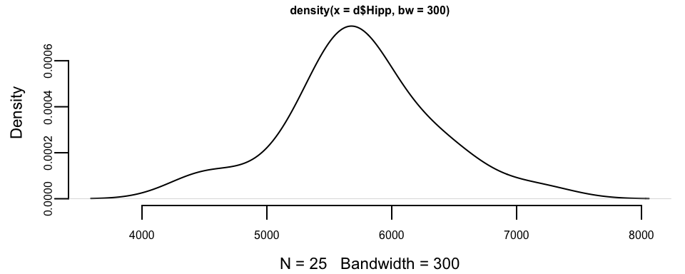
Assume that the hippocampal volumes of the subjects with a history of concussions are independent normal random variables with unknown mean $\mu$ and known standard deviation $\sigma$. Estimate $\sigma$ using the sample standard deviation of the hippocampal volumes (FBConcuss group). Calculate the likelihood for $\mu$.
Assume that $\mu$ has a normal prior distribution with mean $\mu_0$ and standard deviation $\sigma_0$. Estimate those parameters using the sample mean and standard error of the hippocampal volumes across all subjects.
Find the posterior distribution for $\mu$.
Find a 95% posterior credible interval for $\mu$.

Exercise 3.20 (Normal-Normal Chest Measurements) We have chest measurements of 10 000 men. Now, based on memories of my experience as an assistant in a gentlemen’s outfitters in my university vacations, I would suggest a prior \[ \mu \sim N(38, 9). \] Of course, it is open to question whether these men form a random sample from the whole population, but unless I am given information to the contrary I would stick to the prior I have just quoted, except that I might be inclined to increase the variance. My data show that the mean turned out to be 39.8 with a standard deviation of 2.0 for the sample of 10 000.

Calculate the posterior mean for the chest measurements of men in this population
Calculate the predictive distribution for the next observation $x_{n+1}$

Exercise 3.21 (Bayesian Portfolio Updating with Correlated Assets) Coca-Cola (KO) and PepsiCo (PEP) are close competitors whose daily returns are highly correlated, unlike the independent parameter pairs in the Lung Disease and Wolf River problems, where the two groups’ parameters are updated separately. Here you extend the conjugate update from the section Multivariate Normal to the genuinely multivariate case, where the relationship between two parameters must be tracked with a full covariance matrix, as in Example 3.8.

Using quantmod::getSymbols(c("KO","PEP"), from="2015-01-01", to="2023-12-31") and dailyReturn(), compute daily log returns for both stocks. Split the sample into a prior-formation window (2015-01-01 through 2019-12-31, $n_0$ trading days) and a data window (2020-01-01 through 2023-12-31, $n_1$ trading days).
From the prior window compute the sample mean return vector and sample covariance matrix. Specify the prior $\theta \sim N(\mu_0, \Sigma_0)$ for the long-run mean daily returns $\theta=(\theta_{KO}, \theta_{PEP})$, taking $\mu_0$ equal to the prior-window sample mean and $\Sigma_0$ equal to the prior-window sample covariance divided by $n_0$ (the sampling covariance of an estimated mean). Do the same on the data window to get the likelihood $y\mid\theta \sim N(\theta,\Sigma)$.
Apply the multivariate Normal-Normal update to compute the posterior $\theta\mid y \sim N(\mu_1,\Sigma_1)$ with $\Sigma_1=(\Sigma_0^{-1}+\Sigma^{-1})^{-1}$ and $\mu_1 = \Sigma_1(\Sigma_0^{-1}\mu_0 + \Sigma^{-1}y)$. Report the posterior correlation implied by $\Sigma_1$.
Draw 10,000 samples from the joint posterior with MASS::mvrnorm and plot them with the 95% joint credible ellipse (radius $\sqrt{\chi^2_{2,\,0.95}}$ applied through the Cholesky factor of $\Sigma_1$). Mark $\mu_0$, $y$, and $\mu_1$, as in Example 3.8.
Use your posterior draws to estimate $\prob{\theta_{KO} > \theta_{PEP} \mid y}$, the probability that Coca-Cola’s long-run mean daily return exceeds Pepsi’s.
Repeat (c)-(e) but zero out the off-diagonal entries of $\Sigma_0$ and $\Sigma$ before updating (incorrectly treating $\theta_{KO}$ and $\theta_{PEP}$ as independent). Compare the individual posterior standard deviations of $\theta_{KO}$ and $\theta_{PEP}$ with part (c), then compare the resulting $\prob{\theta_{KO} > \theta_{PEP}}$ with part (e). Which comparison changes more, and how does \[ \Var{\theta_{KO} - \theta_{PEP}} = \Var{\theta_{KO}} + \Var{\theta_{PEP}} - 2\,\Cov{\theta_{KO}, \theta_{PEP}} \] explain the pattern?

Exercise 3.22 (Gibbs Sampler) Suppose we model data using the following model \[ \begin{aligned} y_i \sim &N(\mu,\tau^{-1})\\ \mu \sim & N(0,1)\\ \tau \sim & Gamma(2,1). \end{aligned} \]

The goal is to implement a Gibbs sampler for the posterior $\mu,\tau \mid y$, where $y = (y_1,\ldots,y_n)$ is the observed data. The Gibbs sampler iterates between two steps:

Sample $\mu_i$ from $\mu \mid \tau_{i-1}, y$
Sample $\tau_i$ from $\tau_i \mid \mu_i, y$

Show that the full conditional distributions are given by \[ \begin{aligned} \mu \mid \tau, y \sim & N\left(\dfrac{\tau n\bar y}{1+n\tau},\dfrac{1}{1+n\tau}\right)\\ \tau \mid \mu,y \sim & \mathrm{Gamma}\left(2+\dfrac{n}{2}, 1+\dfrac{1}{2}\sum_{i=1}^{n}(y_i-\mu)^2\right) \end{aligned} \]

Use these formulas to implement the Gibbs sampler. The data $y$ is in the file MCMCexampleData.txt.

Plot samples from the joint distribution over $(\mu,\tau)$ on a scatter plot. Plot histograms for marginal $\mu$ and $\tau$.

A thumb tack consists of a short pin with a flat circular head and is used to fasten items such as a piece of paper to a wall or bulletin board. A thumb tack is more interesting for these experimental discussions than a coin, since coins typically have a probability of heads equal to roughly 50%, regardless of the specifics of the coin.↩︎

Name	\(\theta\)	PDF	Mean	Variance	Support
Normal	\(\mu, \sigma^2\)	\(\frac{1}{\sqrt{2\pi\sigma^2}}\exp\left(-\frac{(x-\mu)^2}{2\sigma^2}\right)\)	\(\mu\)	\(\sigma^2\)	\(x \in \mathbb{R}\)
Exponential	\(\lambda\)	\(\lambda e^{-\lambda x}\)	\(\frac{1}{\lambda}\)	\(\frac{1}{\lambda^2}\)	\(x \geq 0\)
Gamma	\(\alpha, \beta\)	\(\frac{\beta^\alpha}{\Gamma(\alpha)}x^{\alpha-1}e^{-\beta x}\)	\(\frac{\alpha}{\beta}\)	\(\frac{\alpha}{\beta^2}\)	\(x \geq 0\)
Poisson	\(\lambda\)	\(\frac{e^{-\lambda}\lambda^x}{x!}\)	\(\lambda\)	\(\lambda\)	\(x \in \mathbb{N}\)
Binomial	\(n, p\)	\(\binom{n}{x}p^x(1-p)^{n-x}\)	\(np\)	\(np(1-p)\)	\(x \in \{0, 1, \ldots, n\}\)
Bernoulli	\(p\)	\(p^x(1-p)^{1-x}\)	\(p\)	\(p(1-p)\)	\(x \in \{0, 1\}\)
Multinomial	\(n, \boldsymbol{p}\)	\(\frac{n!}{x_1!x_2!\cdots x_k!}p_1^{x_1}p_2^{x_2}\cdots p_k^{x_k}\)	\(np_i\)	\(np_i(1-p_i)\)	\(\sum x_i = n, x_i \in \{0,1,\dots,n\}\)
Beta	\(\alpha, \beta\)	\(\frac{\Gamma(\alpha + \beta)}{\Gamma(\alpha)\Gamma(\beta)}x^{\alpha-1}(1-x)^{\beta-1}\)	\(\frac{\alpha}{\alpha + \beta}\)	\(\frac{\alpha\beta}{(\alpha + \beta)^2(\alpha + \beta + 1)}\)	\(x \in [0, 1]\)
Inverse Gamma	\(\alpha, \beta\)	\(\frac{\beta^\alpha}{\Gamma(\alpha)}x^{-\alpha-1}e^{-\frac{\beta}{x}}\)	\(\frac{\beta}{\alpha-1}\)	\(\frac{\beta^2}{(\alpha-1)^2(\alpha-2)}\)	\(x > 0\)

Likelihood	Prior	Prior Parameters	Model Parameters	Sufficient Statistics	Posterior Parameters
Normal (known \(\sigma^2\))	Normal	\(\mu_0, \sigma^2_0\)	\(\mu\)	\(\bar x, n\)	\(\frac{n\sigma^2_0 \bar x + \sigma^2 \mu_0}{\sigma^2 + n\sigma^2_0},~\frac{\sigma^2\sigma_0^2}{n\sigma_0^2+\sigma^2}\)
Normal (known \(\mu\))	Inverse Gamma	\(\alpha,\beta\)	\(\sigma^2\)	\(\sum(x_i-\mu)^2, n\)	\(\alpha+n/2, \beta + \frac{1}{2}\sum(x_i-\mu)^2\)
Binomial (\(m\) trials)	Beta	\(\alpha, \beta\)	\(p\)	\(s, n\)	\(\alpha + s, \beta + nm - s\)
Poisson	Gamma	\(\alpha, \beta\)	\(\lambda\)	\(s, n\)	\(\alpha + s, \beta + n\)
Exponential	Gamma	\(\alpha, \beta\)	\(\lambda\)	\(s, n\)	\(\alpha + n, \beta + s\)
Multinomial	Dirichlet	\(\alpha \in \mathbb{R}^k\)	\(p \in \mathbb{R}^k\)	\(s_j\) for each category \(j\)	\(\alpha+s\)
Normal	Normal-inverse gamma	\(\mu_0, \nu, \alpha, \beta\)	\(\mu, \sigma\)	\(\bar x, \sum(x_i-\bar x)^2, n\)	\(\frac{\nu\mu_0+n\bar{x}}{\nu+n} ,\, \nu+n,\, \alpha+\frac{n}{2} ,\,\) \(\beta + \tfrac{1}{2} \sum_{i=1}^n (x_i - \bar{x})^2 + \frac{n\nu}{\nu+n}\frac{(\bar{x}-\mu_0)^2}{2}\)