17  Model Selection

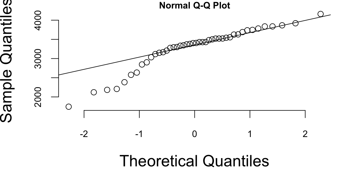
“When you have eliminated the impossible, whatever remains, however improbable, must be the truth.” - Sherlock Holmes

In the world of statistical modeling and machine learning, we face a fundamental challenge that echoes Sherlock Holmes’ famous words about eliminating the impossible to find the truth. When confronted with data, we must navigate through countless possible models, each representing a different hypothesis about the underlying relationships in our data. The art and science of model selection lies in systematically choosing the model that best captures the true signal while avoiding the trap of fitting noise.

In the next chapter (Chapter 18), we focus on regularization techniques, which can also be viewed as model selection mechanisms. Specifically, we discuss Ridge regression, LASSO, and their Bayesian interpretations. These methods offer elegant solutions to the overfitting problem by introducing penalties for model complexity, automatically balancing fit and parsimony. We saw how these frequentist approaches connect to Bayesian thinking through the lens of prior distributions and posterior inference.

This chapter explores the critical decisions involved in choosing the right model. We begin by examining the fundamental considerations that guide model selection: the bias-variance tradeoff, the challenges of overfitting and underfitting, and the practical constraints of computational resources and data quality. We’ll explore how the purpose of our analysis—whether prediction or interpretation—should influence our modeling choices, drawing on Leo Breiman’s influential distinction between the “two cultures” of statistical modeling.

The chapter then delves into practical methodologies for model evaluation and selection. We’ll cover exploratory data analysis techniques that help us understand our data before committing to a particular model form, followed by rigorous approaches to measuring out-of-sample performance through cross-validation and information criteria. These tools provide the foundation for making principled decisions about model complexity.

By the end of this chapter, you’ll have a comprehensive toolkit for approaching model selection problems, understanding when different techniques are appropriate, and implementing these methods in practice. Most importantly, you’ll develop the judgment to balance the competing demands of accuracy, interpretability, and computational efficiency that characterize real-world modeling challenges.

17.1 Fundamental Considerations in Model Selection

When building predictive models, several important considerations guide our choices. Understanding these factors helps us make informed decisions about model complexity and selection.

Model Complexity and Generalization: Choosing the right model for the relationship between \(x\) and \(y\) involves navigating a fundamental trade-off between model complexity and generalization ability. If the chosen model is too simple (e.g., linear regression when the true relationship is polynomial), it might underfit the data and fail to capture important relationships, leading to high bias and poor performance on both training and test data. Conversely, a model that is too complex (e.g., high-degree polynomials or deep neural networks with insufficient data) might overfit the data by memorizing training examples rather than learning the underlying pattern, resulting in excellent training performance but poor generalization to unseen examples. This problem becomes even more complex when dealing with non-linear relationships, high-dimensional data, or noisy data, where the optimal model complexity is not immediately obvious and may require systematic experimentation with different model architectures, regularization techniques, and hyperparameter tuning to find the right balance between capturing the true signal while avoiding noise.

Overfitting and Underfitting: Overfitting occurs when the model fits the training data too closely, capturing not only the true underlying relationship but also random noise and idiosyncrasies specific to the training dataset. This phenomenon typically manifests when a model has too many parameters relative to the amount of training data available, allowing it to essentially “memorize” the training examples rather than learning the generalizable patterns. The model may achieve excellent performance metrics on the training data (low training error) but will perform poorly on new, unseen data (high generalization error). This is because the model has learned to recognize specific noise patterns in the training data that don’t exist in the broader population. Common signs of overfitting include a large gap between training and validation/test performance, or performance that improves on training data while degrading on validation data during training iterations.

Underfitting occurs when the model is too simple and fails to capture the true relationship between \(x\) and \(y\), often due to insufficient model complexity or inadequate training. This can happen when using a model that is inherently too simple for the problem at hand (e.g., linear regression for a highly non-linear relationship), when the model hasn’t been trained for enough iterations, or when regularization is applied too aggressively. Underfitting results in poor performance on both training and test data, as the model lacks the capacity to learn the underlying patterns in the data. The model essentially misses important features or relationships that are necessary for accurate predictions. Unlike overfitting, underfitting typically shows similar poor performance across training, validation, and test sets, indicating that the model is not capturing the signal in the data regardless of the dataset.

Data Quality and Quantity: The accuracy of predictions heavily relies on the quality and quantity of the available data. If the data is noisy, inaccurate, or incomplete, it can lead to misleading predictions. A sufficient amount of data is also crucial to ensure the model can learn the underlying relationship effectively. Insufficient data can result in underfitting and poor generalization.

Data quality issues can manifest in various forms, including missing values, inconsistent formatting, labeling errors, and biased sampling. These problems are particularly acute in machine learning applications where large volumes of labeled data are required for training. To address these challenges, companies have emerged that specialize in data quality improvement and annotation services.

Companies like Scale AI and Toloka provide platforms that help organizations improve data quality through human-in-the-loop annotation and validation processes. These platforms employ large networks of human annotators who can perform tasks such as image labeling, text classification, data validation, and quality control. Scale AI, for example, offers services for creating high-quality training datasets through human annotation, with built-in quality control mechanisms that include multiple annotators per task and consensus-based validation. Their platform can handle various data types including images, text, and video, making it suitable for computer vision, natural language processing, and other AI applications.

Toloka, similarly, provides a crowdsourcing platform that connects businesses with a global network of contributors who can perform data labeling, content moderation, and quality assessment tasks. Their platform includes quality control features such as skill-based routing, where tasks are assigned to annotators based on their demonstrated expertise, and dynamic overlap, where multiple workers verify the same data to ensure accuracy.

These platforms help address several key data quality challenges: they can identify and correct labeling errors through consensus mechanisms, handle missing data through targeted collection efforts, and ensure consistency in data formatting and annotation standards. By leveraging human expertise at scale, these services enable organizations to create more reliable training datasets, which in turn leads to better-performing machine learning models and more accurate predictions.

Model Explainability: In many applications, it is crucial to understand how the model arrives at its predictions. This is particularly important in areas like healthcare or finance, where transparency and interpretability are essential. Some models, particularly complex ones like deep neural networks, can be difficult to interpret, making it challenging to understand the rationale behind their predictions. However, modern machine learning has developed several techniques to address this challenge and make complex models more interpretable.

The importance of explainability extends beyond mere curiosity about model behavior. In healthcare applications, doctors need to understand why a model recommended a particular diagnosis or treatment plan to make informed decisions and maintain trust in the system. A model that predicts a patient has a 90% chance of having cancer but cannot explain which symptoms or test results led to this conclusion would be of limited clinical value. Similarly, in financial services, regulators require explanations for credit decisions to ensure compliance with fair lending laws and to prevent discriminatory practices. When a loan application is denied, both the applicant and regulatory bodies need to understand the specific factors that influenced this decision.

In legal and compliance contexts, explainability becomes a legal requirement. The European Union’s General Data Protection Regulation (GDPR) includes a “right to explanation” that allows individuals to request information about automated decisions that affect them. This has created a legal imperative for organizations to develop explainable AI systems. In criminal justice applications, where AI systems might be used for risk assessment or sentencing recommendations, the stakes are particularly high. Judges, lawyers, and defendants all need to understand how these systems arrive at their conclusions to ensure fair and just outcomes.

One prominent approach is the use of interpretable surrogate models, such as LIME (Local Interpretable Model-agnostic Explanations) and SHAP (SHapley Additive exPlanations). These methods work by approximating the complex model’s behavior in the vicinity of a specific prediction using simpler, more interpretable models like linear regression or decision trees. LIME, for instance, creates local explanations by sampling points around the prediction of interest and fitting a linear model to explain the model’s behavior in that neighborhood. This allows us to understand which features contributed most to a particular prediction, even for complex models like deep neural networks.

Another powerful technique is attention mechanisms, which have become increasingly popular in natural language processing and computer vision. Attention mechanisms allow models to “focus” on specific parts of the input when making predictions, providing a form of built-in interpretability. For example, in image classification tasks, attention maps can highlight which regions of an image the model is focusing on when making its prediction, making it easier to understand the model’s decision-making process.

Gradient-based methods offer another approach to model interpretability. Techniques like Grad-CAM (Gradient-weighted Class Activation Mapping) use gradients to identify which parts of the input are most important for the model’s prediction. By computing the gradient of the model’s output with respect to the input features, these methods can create heatmaps that show which features or regions contributed most to the final prediction.

For tree-based models like random forests and gradient boosting machines, built-in feature importance measures provide natural interpretability. These methods can rank features based on their contribution to the model’s predictive performance, offering insights into which variables are most important for making predictions.

Model distillation techniques represent another approach, where a complex model (the teacher) is used to train a simpler, more interpretable model (the student) that mimics the teacher’s behavior. The student model, being simpler, is easier to interpret while maintaining much of the teacher’s predictive performance.

Finally, counterfactual explanations provide a different type of interpretability by showing what changes to the input would be needed to change the model’s prediction. For example, if a loan application is rejected, a counterfactual explanation might show that the application would have been approved if the applicant’s income were $10,000 higher or if their credit score were 50 points better.

These modern interpretability techniques have made it possible to understand and explain the behavior of even the most complex models, addressing the “black box” problem that has historically limited the adoption of advanced machine learning methods in critical applications where transparency is essential.

Computational Cost: Training and using prediction models can be computationally expensive, especially for complex models with large datasets. This can limit their applicability in resource-constrained environments. Finding a balance between model complexity, accuracy, and computational cost is critical for practical applications.

The computational demands of machine learning models have been significantly addressed through the development of specialized hardware, particularly Graphics Processing Units (GPUs). Originally designed for rendering graphics in video games, GPUs have become essential for deep learning due to their parallel processing architecture. Unlike traditional Central Processing Units (CPUs) that process tasks sequentially, GPUs can perform thousands of mathematical operations simultaneously, making them ideal for the matrix multiplications and tensor operations that are fundamental to neural network training. This parallel processing capability has reduced training times from weeks to hours or even minutes for many deep learning models, democratizing access to advanced machine learning techniques.

However, the computational cost challenge extends beyond just training to the deployment phase, where models need to run efficiently in production environments. This has led to the emergence of edge computing as a crucial solution. Edge computing involves processing data and running models closer to where the data is generated, rather than sending everything to centralized cloud servers. This approach offers several advantages for machine learning applications: reduced latency for real-time predictions, lower bandwidth costs by processing data locally, and improved privacy by keeping sensitive data on local devices.

Edge computing is particularly important for applications requiring real-time decision making, such as autonomous vehicles, industrial IoT systems, and mobile applications. For example, a self-driving car cannot afford the latency of sending sensor data to a cloud server and waiting for predictions to return; it needs to process information and make decisions locally within milliseconds. Similarly, smart manufacturing systems use edge computing to monitor equipment and predict maintenance needs in real-time without the delays associated with cloud processing.

Quantization and lower precision calculations have emerged as powerful techniques for reducing computational costs while maintaining model performance. Traditional neural networks use 32-bit floating-point numbers (FP32) for all calculations, which provides high precision but requires significant computational resources and memory. Quantization reduces the precision of these numbers, typically to 16-bit (FP16), 8-bit integers (INT8), or even 4-bit integers (INT4), dramatically reducing both memory usage and computational requirements. For example, converting from FP32 to INT8 can reduce memory usage by 75% and computational cost by 2-4x, while often maintaining acceptable accuracy levels. This is particularly valuable for deployment on edge devices with limited resources, such as smartphones, IoT devices, and embedded systems. Modern hardware, including specialized AI accelerators like Google’s Tensor Processing Units (TPUs) and NVIDIA’s Tensor Cores, are specifically designed to handle these lower precision calculations efficiently, further reducing the computational cost barrier.

The trade-offs between computational cost and model performance are becoming increasingly sophisticated. Techniques like model pruning, which removes unnecessary connections from neural networks, can create smaller, faster models. Knowledge distillation allows large, complex models to transfer their knowledge to smaller, more efficient models that can run on resource-constrained devices.

These developments have created a spectrum of deployment options, from powerful cloud-based systems that can run the most complex models to lightweight edge devices that can perform basic predictions locally. The choice depends on the specific requirements of the application, including latency requirements, accuracy needs, privacy concerns, and cost constraints. As hardware continues to improve and optimization techniques become more sophisticated, the computational cost barrier to deploying machine learning models continues to decrease, opening up new possibilities for AI applications in previously inaccessible domains.

Ethical Considerations: Predictions can have significant real-world consequences, raising ethical concerns about bias, fairness, and potential misuse. It is crucial to consider the potential harms and unintended consequences of predictions and implement safeguards to mitigate them.

The ethical implications of predictive models have become increasingly prominent as these systems are deployed in critical domains such as healthcare, criminal justice, employment, and financial services. One of the most significant concerns is algorithmic bias, which can perpetuate or amplify existing societal inequalities. For example, facial recognition systems have been shown to have higher error rates for people of color, potentially leading to wrongful arrests or surveillance. Similarly, hiring algorithms trained on historical data may perpetuate gender or racial biases present in past hiring decisions, creating a feedback loop that reinforces discrimination.

Fairness in machine learning has emerged as a critical research area, with multiple definitions and approaches to ensure equitable treatment across different demographic groups. Statistical parity, equalized odds, and individual fairness are among the various fairness metrics that can be applied depending on the specific context and requirements of the application. However, achieving fairness often involves trade-offs with model accuracy, and different fairness definitions may conflict with each other, requiring careful consideration of which definition is most appropriate for a given use case.

The potential for misuse of predictive models is another significant concern. Models designed for legitimate purposes can be repurposed for harmful applications, such as using facial recognition for mass surveillance or employing predictive policing algorithms that disproportionately target certain communities. Additionally, the increasing sophistication of deepfake technology, which uses predictive models to generate realistic but fake images, videos, or audio, raises concerns about misinformation and manipulation.

Privacy concerns arise when predictive models require access to sensitive personal data. The collection, storage, and processing of personal information for training and deploying these models can violate individual privacy rights and create risks of data breaches. Differential privacy techniques, which add carefully calibrated noise to data or model outputs, have emerged as a promising approach to protect individual privacy while maintaining model utility.

Transparency and accountability are essential for addressing ethical concerns. Organizations deploying predictive models must be able to explain their decisions and be held accountable for any harms that result. This includes maintaining audit trails, implementing human oversight mechanisms, and establishing clear procedures for addressing complaints or errors. The concept of “algorithmic impact assessments” has been proposed as a framework for evaluating the potential social impacts of automated decision-making systems before deployment.

Regulatory frameworks are evolving to address these ethical challenges. The European Union’s General Data Protection Regulation (GDPR) includes provisions for automated decision-making and profiling, while various jurisdictions are developing specific regulations for AI systems. These regulations often require transparency, human oversight, and the ability to contest automated decisions.

Technical approaches to addressing ethical concerns include adversarial training to reduce bias, interpretability techniques to increase transparency, and robust testing procedures to identify potential harms before deployment. Regular monitoring and updating of deployed models is also crucial, as societal norms and legal requirements evolve over time.

Addressing these challenges requires careful consideration of the specific problem, selection of appropriate techniques, and continuous evaluation and improvement of the prediction model. It also requires collaboration between technical experts, domain specialists, ethicists, and stakeholders to ensure that predictive models serve the public good while minimizing potential harms.

17.2 Prediction vs Interpretation

Predictive models can serve two distinct purposes: prediction and interpretation. While these goals are not mutually exclusive, they often conflict with each other. The goal of interpretation is to understand the relationship between the input and output variables, which typically requires simpler, more transparent models.

A model that excels at prediction might not be suitable for interpretation. For example, a complex deep neural network might achieve high predictive accuracy but provide little insight into how the input variables influence the output. Conversely, a simple linear model might be highly interpretable but lack the flexibility to capture complex relationships in the data. A key advantage of linear models is their ability to serve both purposes effectively, unlike more complex models with many parameters that can be difficult to interpret.

Interpretation problems typically require simpler models. We prioritize models that are easy to interpret and explain, even if they have slightly lower predictive accuracy. The evaluation metrics also differ: for interpretation, we typically use the coefficient of determination (R-squared) or p-values, which provide insights into the model’s fit and the statistical significance of the estimated relationships.

The choice between using a model for prediction or interpretation depends on the specific task and desired outcome. If the primary goal is accurate predictions, a complex model with high predictive accuracy might be preferred, even if it is less interpretable. However, if understanding the underlying relationships and causal mechanisms is crucial, a simpler and more interpretable model might be chosen, even if it has slightly lower predictive accuracy. Interpretive models are commonly used in scientific research, social sciences, and other fields where understanding the underlying causes and relationships is crucial.

In practice, it’s often beneficial to consider both prediction and interpretation when building and evaluating models. However, it is not unusual to build two different models, one for prediction and one for interpretation. This allows for a more nuanced analysis of the data and can lead to better insights than using a single model for both purposes.

Breiman’s Two Cultures

Let \(x\) be a high-dimensional input containing a large set of potentially relevant data, and let \(y\) represent an output (or response) to a task that we aim to solve based on the information in \(x\). Breiman [2000] summarizes the difference between statistical and machine learning philosophy as follows:

“There are two cultures in the use of statistical modeling to reach conclusions from data. One assumes that the data are generated by a given stochastic data model. The other uses algorithmic models and treats the data mechanism as unknown.”

“The statistical community has been committed to the almost exclusive use of data models. This commitment has led to irrelevant theory, questionable conclusions, and has kept statisticians from working on a large range of interesting current problems.”

“Algorithmic modeling, both in theory and practice, has developed rapidly in fields outside statistics. It can be used both on large complex data sets and as a more accurate and informative alternative to data modeling on smaller data sets. If our goal as a field is to use data to solve problems, then we need to move away from exclusive dependence on data models and adopt a more diverse set of tools.”

This distinction highlights the fundamental difference between the traditional statistical approach, which assumes a specific data-generating process, and the machine learning approach, which focuses on finding patterns in data without making strong assumptions about the underlying mechanism.

Statistical prediction problems are of great practical and theoretical interest. Deep learning predictors offer several advantages over traditional predictors:

• Input data can include all data of possible relevance to the prediction problem at hand
• Nonlinearities and complex interactions among input data are accounted for seamlessly
• Overfitting is more easily avoided than with traditional high-dimensional procedures
• Fast, scalable computational frameworks (such as TensorFlow) are available

Tree-based models and deep learning models exemplify the “algorithmic culture” that Breiman describes. These models can capture complex, non-linear relationships in data without requiring explicit specification of the functional form. However, this flexibility comes at the cost of interpretability. While decision trees offer some interpretability through their hierarchical structure, deep neural networks are often considered “black boxes” due to their complex, multi-layered architecture.

The trade-off between interpretability and accuracy is a central theme in modern machine learning. Simple models like linear regression are highly interpretable but may lack the flexibility to capture complex patterns. Complex models like deep neural networks can achieve high accuracy but are difficult to interpret. This has led to the development of various techniques for making complex models more interpretable, including feature importance measures, attention mechanisms, and surrogate models that approximate the behavior of complex models with simpler, more interpretable ones.

17.3 What Makes a Good Predictive Model?

What makes a good model? If the goal is prediction, then the model is as good as its predictions. The easiest way to visualize the quality of predictions is to plot \(y\) versus \(\hat{y}\). Most of the time we use empirical assessment of model quality. However, sometimes theoretical bounds can be derived for a model that describe its accuracy. For example, in the case of the linear regression model, the prediction interval is defined by \[ \hat{y} \pm s\sqrt{1+\frac{1}{n}+\frac{(x-\bar{x})^2}{\sum_{i=1}^n(x_i-\bar{x})^2}} \] where \(s\) is the standard deviation of the residuals. The prediction interval is the confidence interval for the prediction. The prediction interval is wider than the confidence interval because it includes the uncertainty in the prediction.

Assume we have a predictive model \[ y = f(x) + \epsilon \] and we have some modeling assumption regarding the distribution of \(\epsilon\). For example, when we use linear regression or BART, we assume that \(\epsilon\) follows a normal distribution. One simple approach to test if observed samples \(\epsilon_1,\ldots,\epsilon_n\) follow a specific distribution is to use Exploratory Data Analysis (EDA).

The most common tools for exploratory data analysis are Q-Q plots, scatter plots, and bar plots/histograms.

A Q-Q plot compares the quantiles of your data with the quantiles of a theoretical distribution (like normal, exponential, etc.). A quantile is the fraction (or percent) of points below the given value. That is, the \(i\)-th quantile is the point \(x\) for which \(i\)% of the data lies below \(x\). On a Q-Q plot, if the two datasets come from a population with the same distribution, we should see the points forming a line that’s roughly straight. More precisely, if the two datasets \(x\) and \(y\) come from the same distribution, then the points \((x_{(i)}, y_{(i)})\) should lie roughly on the line \(y = x\). If \(y\) comes from a distribution that’s linear in \(x\), then the points \((x_{(i)}, y_{(i)})\) should lie roughly on a line, but not necessarily on the line \(y = x\).

Example 17.1 (Normal Q-Q plot) Figure 17.1 shows the normal Q-Q plot for the Data on birth weights of babies born in a Brisbane hospital on December 18, 1997. The data set contains 44 records. A more detailed description of the data set can be found in UsingR manual.

babyboom = read.csv("../data/babyboom.csv")
qqnorm(babyboom$wt, bg="lightblue"); qqline(babyboom$wt, col="red", lwd=3)

Figure 17.1: Normal Q-Q plot of baby weights

Visually, the answer to the question “Are Birth Weights Normally Distributed?” is no. We can see that on the left side of the plot the points are below the line. This indicates that the data is skewed to the left. The data is not normally distributed.

The Q-Q plots look different if we split the data based on the gender

par(mar=c(4,4,0.7,0.5), bty='n', cex.lab=1, cex.axis=0.5,cex.main=0.5,pch=21,cex=1.3)
g = babyboom %>% filter(gender=="girl") %>% pull(wt) 
b = babyboom %>% filter(gender=="boy") %>% pull(wt) 
qqnorm(g, bg="lightblue"); qqline(g, col=2)
qqnorm(b, bg="lightblue"); qqline(b, col=2)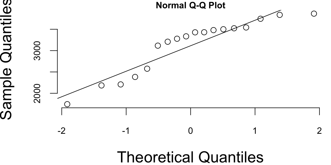

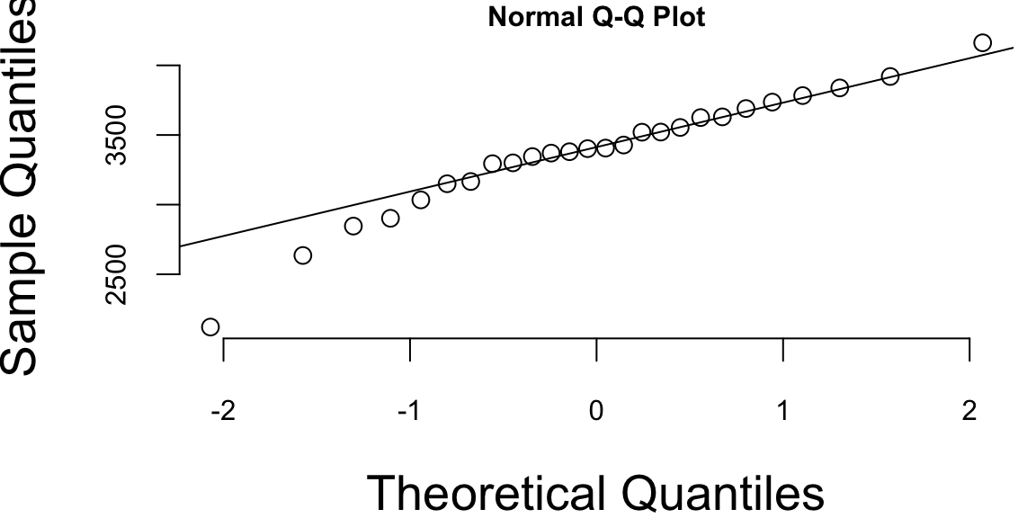
Girls

Boys

Histogram of baby weights by gender

How about the times in hours between births of babies?

hr = ceiling(babyboom$running.time/60)
BirthsByHour = tabulate(hr)
# Number of hours with 0, 1, 2, 3, 4 births
ObservedCounts = table(BirthsByHour) 
# Average number of births per hour
BirthRate=sum(BirthsByHour)/24    
# Expected counts for Poisson distribution
ExpectedCounts=dpois(0:4,BirthRate)*24    
# bind into matrix for plotting
ObsExp <- rbind(ObservedCounts,ExpectedCounts) 
barplot(ObsExp,names=0:4, beside=TRUE,legend=c("Observed","Expected"))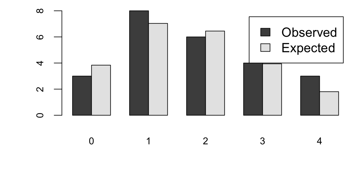

What about the Q-Q plot?

# birth intervals
birthinterval=diff(babyboom$running.time) 
 # quantiles of standard exponential distribution (rate=1)   
exponential.quantiles = qexp(ppoints(43)) 
qqplot(exponential.quantiles, birthinterval, bg="lightblue")
lmb=mean(birthinterval)
lines(exponential.quantiles,exponential.quantiles*lmb, col=2) # Overlay a line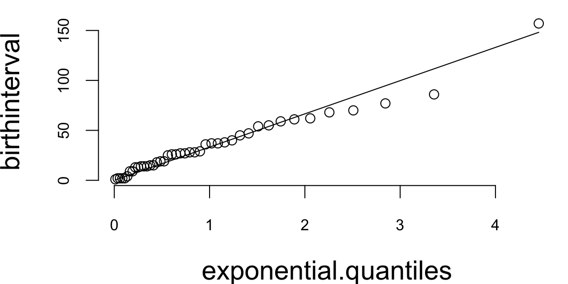

Here

• ppoints function computes the sequence of probability points
• qexp function computes the quantiles of the exponential distribution
• diff function computes the difference between consecutive elements of a vector

17.4 Out-of-Sample Performance

A parametric model that we choose to fit to data is selected from a family of functions. We then use optimization to find the best model from that family by either minimizing empirical loss or maximizing the likelihood. Finding an appropriate family of functions is a major problem called the model selection problem. For example, the choice of input variables to be included in the model is part of the model selection process. Model selection involves determining which predictors, interactions, or transformations should be included in the model to achieve the best balance between complexity and predictive accuracy. In practice, we often encounter several models for the same dataset that perform nearly identically, making the selection process challenging.

It is important to note that a good model is not necessarily the one that fits the data perfectly. Overfitting can occur when a model is overly complex, capturing noise rather than the underlying pattern. A good model strikes a balance between fitting the data well and maintaining simplicity to ensure generalizability to new, unseen data. For instance, including too many parameters can lead to a perfect fit when the number of observations equals the number of parameters, but such a model is unlikely to perform well on out-of-sample data.

The goal of model selection is not only to achieve a good fit but also to reduce complexity by excluding unnecessary parameters. This process typically involves selecting a model from a relevant class of functions while keeping in mind the trade-offs between bias, variance, and model complexity. Techniques such as cross-validation, information criteria (e.g., AIC, BIC), and regularization methods are commonly used to guide the model selection process.

The model selection task is sometimes one of the most time-consuming parts of data analysis. Unfortunately, there is no single rule to find the best model. One way to think about the model choice problem is as yet another optimization problem, with the goal of finding the best family of functions that describe the data. With a small number of predictors, we can use brute force (check all possible models). For example, with \(p\) predictors there are \(2^p\) possible models with no interactions. Thus, the number of potential function families is huge even for modest values of \(p\). One cannot consider all transformations and interactions.

Our goal is to build a model that predicts well for out-of-sample data, i.e., data that was not used for training. Ultimately, we are interested in using our models for prediction, and thus out-of-sample performance is the most important metric and should be used to choose the final model. In-sample performance is of little interest when choosing a predictive model, as one of the winners of the Netflix prize put it: “It’s like predicting how much someone will like a movie, having them watch it and tell you how much they really liked it.” Out-of-sample performance is the final judge of the quality of our model. The goal is to use data to find a pattern that we can exploit. The pattern will be “statistical” in nature. To uncover the pattern, we start with a training dataset, denoted by \[ D = (y_i,x_i)_{i=1}^n \] and to test the validity of our model, we use an out-of-sample testing dataset \[ D^* = (y_j^*, x_j^*)_{j=1}^m, \] where \(x_i\) is a set of \(p\) predictors and \(y_i\) is the response variable.

A good predictor will “generalize” well and provide low MSE out-of-sample. There are a number of methods/objective functions that we will use to find \(\hat{f}\). In a parameter-based approach, we will find a black box. There are a number of ways to build our black box model. Our goal is to find the map \(f\) that approximates the process that generated the data. For example, data could represent some physical observations, and our goal is to recover the “laws of nature” that led to those observations. One of the pitfalls is to find a map \(f\) that does not generalize. Generalization means that our model actually learned the “laws of nature” and not just identified patterns present in training. The lack of generalization of the model is called overfitting. It can be demonstrated in one dimension by remembering the fact from calculus that any set of \(n\) points can be approximated by a polynomial of degree \(n\), e.g., we can always draw a line that connects two points. Thus, in one dimension we can always find a function with zero empirical risk. However, such a function is unlikely to generalize to observations that were not in our training data. In other words, the empirical risk measure for \(D^*\) is likely to be very high. Let us illustrate that in-sample fit can be deceiving.

Example 17.2 (Hard Function) Say we want to approximate the following function \[ f(x) = \dfrac{1}{1+25x^2}. \] This function is simply a ratio of two polynomial functions and we will try to build a linear model to reconstruct this function

x = seq(-2,2,by=0.01)
y = 1/(1+25*x^2)
# Approximate with polynomial of degree 1 and 2
m1 = lm(y~x)
m2 = lm(y~poly(x,2))
# Approximate with polynomial of degree 20 and 5
m20 = lm(y~poly(x,20))
m5 = lm(y~poly(x,5))
x = seq(-3,3,by=0.01)
y = 1/(1+25*x^2)
plot(x,y,type='l',col='black',lwd=2)
lines(x,predict(m1,list(x=x)),lwd=2, col=1)
lines(x,predict(m2,poly(x,2)),lwd=2, col=2)
lines(x,predict(m5,poly(x,5)),lwd=2, col=3)
lines(x,predict(m20,poly(x,20)),lwd=2, col=4)
legend("topright", legend=c("f(x)","m1","m2","m5","m20"), col=c("black",1:4), lty=1, cex=0.8, bty='n')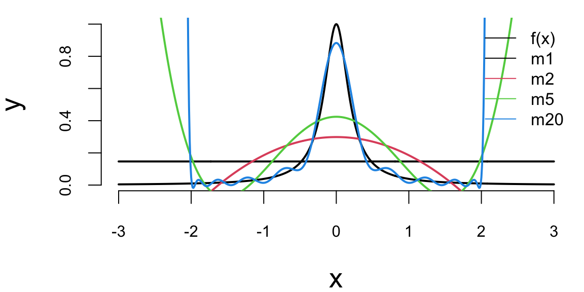

Figure 17.2: Runge-Kutta function

Figure 17.2 shows the function itself (black line) on the interval \([-3,3]\). We used observations of \(x\) from the interval \([-2,2]\) to train the data (solid line) and from \([-3,-2) \cup (2,3]\) (dotted line) to test the model and measure the out-of-sample performance. We tried four different linear functions to capture the relations. We see that linear model \(\hat{y} = \beta_0 + \beta_1 x\) is not a good model. However, as we increase the degree of the polynomial to 20, the resulting model \(\hat{y} = \beta_0 + \beta_1x + \beta_2 x^2 +\ldots+\beta_{20}x^{20}\) does fit the training dataset quite well, but does a very poor job on the test dataset. Thus, while in-sample performance is good, the out-of-sample performance is unsatisfactory. We should not use the degree 20 polynomial function as a predictive model. In practice, in-sample loss or classification rates provide us with a metric for comparing different predictors. It is worth mentioning here that there should be a penalty for overly complex rules that fit extremely well in-sample but perform poorly on out-of-sample data. As Einstein famously said, “A model should be simple, but not simpler.”

To a Bayesian, the solution to these decision problems are rather obvious: compute posterior distributions, and then make decisions by maximizing expected utility, where the posterior distribution is used to calculate the expectations. Classical solutions to these problems are different, and use repeated sampling ideas, whereby the performance of a decision rule is judged on its performance if the same decision problem were repeated infinitely. Thus, the decisions are made based on their population properties. One of the main uses of statistical decision theory is to compare different estimators or hypothesis testing procedures. This theory generates many important findings, most notably that many of the common classical estimators are “bad”,in some sense, and that Bayesian estimators are always “good”.

These results have major implications for empirical work and practical applications, as they provide a guide for forecasting.

17.5 Bias-Variance Trade-off

For any predictive model, we seek to achieve the best possible results, i.e., the smallest MSE or misclassification rate. However, model performance can vary depending on the specific training/validation split used. A model that performed well on one test set may not produce good results given additional data. Sometimes we observe situations where a small change in the data leads to a large change in the final estimated model, e.g., the parameters of the model. These results exemplify the bias/variance tradeoff, where increasing model bias can reduce variance in the final results. Similarly, low bias can result in high variance, but can also produce an oversimplification of the final model. The bias/variance concept is depicted below.

Figure 17.3: Bias-variance trade-off

Example 17.3 (Bias-variance) We demonstrate bias-variance concept using Boston housing example. We fit a model \(\mathrm{medv} = f(\mathrm{lstat})\). We use polynomial functions to approximate this relation. We fitted twelve polynomial functions with degree \(1,\ldots,12\) ten time. Each time we randomly selected 20% of sample for testing and the rest for training. We estimated in-of-sample performance (bias) and out-of-sample performance by calculating MSE on training and testing sets correspondingly. For each polynomial \(f\) we averaged MSE from each of the ten models.

Figure 17.4 (a) shows bias and variance for our twelve different models. As expected, bias increases while variance decreases as model complexity grows. On the other hand out-of-sample MSE is a U-shaped curve. The optimal model is the one that has smallest out-of-sample MSE. In our case it is polynomial of degree 5!

(a) Metrics for twelve polynomial functions fitted into Boston housing data set. As model complexity (degree of the polynomial function) increases, model variance increase and bias decreases. Out-of-sample MSE is smallest for 5th degree polynomial function, which is the optimal model in terms of bias-variance trade-off.

(b) Optimal complexity model, which is 5th degree polynomial used to predict observations from testing data set. Model predictions (red line) are compared to actual observed values of medv variable (dots)

Figure 17.4: Metrics for 12 models

Let’s take another, more formal look at the bias-variance trade-off for a linear regression problem. We are interested in the decomposition of the error \(\E{(y-\hat{y})^2}\) as a function of bias \(\E{y-\hat{y}}\) and variance \(\Var{\hat{y}}\).

Here \(\hat{y} = \hat{f}_{\beta}(x)\) is the prediction from the model, and \(y = f(x) + \epsilon\) is the true value, which is measured with noise \(\Var{\epsilon} = \sigma^2\), where \(f(x)\) is the true unknown function. The expectation above measures the squared error of our model on a random sample \(x\). \[ \begin{aligned} \E{(y - \hat{y})^2} & = \E{y^2 + \hat{y}^2 - 2 y\hat{y}} \\ & = \E{y^2} + \E{\hat{y}^2} - \E{2y\hat{y}} \\ & = \Var{y} + \E{y}^2 + \Var{\hat{y}} + \E{\hat{y}}^2 - 2f\E{\hat{y}} \\ & = \Var{y} + \Var{\hat{y}} + (f^2 - 2f\E{\hat{y}} + \E{\hat{y}}^2) \\ & = \Var{y} + \Var{\hat{y}} + (f - \E{\hat{y}})^2 \\ & = \sigma^2 + \Var{\hat{y}} + \mathrm{Bias}(\hat{y})^2\end{aligned} \] Here we used the following identity: \(\Var{X} = \E{X^2} - \E{X}^2\) and the fact that \(f\) is deterministic and \(\E{\epsilon} = 0\), thus \(\E{y} = \E{f(x)+\epsilon} = f + \E{\epsilon} = f\).

17.6 Cross-Validation

If the dataset at hand is small and we cannot dedicate a large enough sample size for testing, simply measuring error on a test dataset can lead to wrong conclusions. When the size of the testing set \(D^*\) is small, the estimated out-of-sample performance has high variance, depending on precisely which observations are included in the test set. On the other hand, when the training set \(D^*\) is a large fraction of the entire sample available, the estimated out-of-sample performance will be underestimated. Why?

A simple solution is to perform the training/testing split randomly several times and then use the average out-of-sample errors. This procedure has two parameters: the fraction of samples to be selected for testing \(p\) and the number of estimates to be performed \(K\). The resulting algorithm is as follows:

fsz = as.integer(p*n)
error = rep(0,K)
for (k in 1:K)
{
    test_ind = sample(1:n,size = fsz)
    training = d[-test_ind,]
    testing = d[test_ind,]
    m = lm(y~x, data=training)
    yhat = predict(m,newdata = testing)
    error[k] = mean((yhat-testing$y)^2)
}
res = mean(error)

Figure 17.5 shows the process of splitting the dataset randomly five times.

Cross-validation modifies the random splitting approach to use a more “disciplined” way to split the dataset for training and testing. Instead of randomly selecting training data points, CV chooses consecutive observations, and thus each data point is used once for testing. Like the random approach, CV helps address the high variance issue of out-of-sample performance estimation when the available dataset is small. Figure 17.6 shows the process of splitting the dataset five times using the cross-validation approach.

Figure 17.5: Bootstrap

Figure 17.6: Cross-validation

Training set (red) and testing set (green)

Example 17.4 (Simulated) We use simulated data set to demonstrate difference between estimated out-of-sample performance using random 20/80 split, 5-fold cross-validation and random split. We used \(x=-2,-1.99,-1.98,\ldots,2\) and \(y = 2+3x + \epsilon, ~ \epsilon \sim N(0,\sqrt{3})\). We simulated 35 datasets of size 100. For each of the simulated data sets, we fitted a linear model and estimated out-of-sample performance using three different approaches. Figure 17.7 compares empirical distribution of errors estimated from 35 samples.

Figure 17.7: Empirical comparison of simple split, cross-validation, and bootstrap approaches to estimate out-of sample performance.

As we can see the estimated out-of-sample performance by a training set approach is of high variance. While, both cross-validation and bootstrap approaches lead to better estimates, they require model to be fitted 5 times, which can be computationally costly for a complex model. On the other hand, estimate from cross-validation is of lower variance and less bias compared to the bootstrap estimate. Thus, we should prefer cross-validation.

17.7 Bayesian Model Selection

The probabilistic models of interest are the joint probability distribution \(p(D,\theta)\) (called a generative model) and \(P(Y,\theta \mid X)\) (discriminative model). Discriminative models are easier to build and are more frequently used in practice. Generative models require modeling a distribution over the set of observed variables, which makes our model more complicated. Text analysis provides an illustrative example. The task of identifying the topic of an article can be solved using a discriminative distribution. The problem of generating a new article requires a generative model.

Let \(D\) denote data. Let \(\theta_M \in \Theta_M\) denote a set of parameters under model \(M \in \mathcal{M}\). Let \(\theta_M = (\theta_1, \ldots, \theta_M)\) be the \(p\)-vector of parameters. The Bayesian approach is straightforward: implement the Bayesian paradigm by executing Bayes’ rule. This requires the laws of probability and not optimization techniques. The notion of model complexity is no different. Let \(\mathcal{M}\) denote the space of models and \(\theta\) be the parameter vector. The Bayesian paradigm simply places probabilities over parameters and models given the data, namely \(p(\theta_M, M \mid y)\), where \(y = (y_1, \ldots, y_n)\).

This has a number of decompositions. Bayes’ theorem calculates the joint posterior over parameters and models given data \(D\), namely \[ P(\theta_M,M\mid D) = P(\theta_M \mid M,D)P(M\mid D). \] Notice how this factors the posterior into two terms: the conditional posterior over parameters given the model and the posterior over models given data.

The key quantity is the weight of evidence (a.k.a. marginal distribution of the data \(D\) given the model \(M\)), defined by \[ p(D \mid M) = \int_{\Theta_M} p(D \mid \theta_M, M) p(\theta_M \mid M) d\theta_M. \] Here \(p(D \mid \theta_M, M)\) is the traditional likelihood function. The key conditional distribution, however, is the specification of the prior over parameters \(p(\theta_M \mid M)\). As this is used in the marginalization, it can affect the Bayes risk dramatically. Occam’s razor comes from the fact that this marginalization provides a weight of evidence that favors simpler models over more complex ones.

This leads to a posterior over models, which is calculated as: \[\begin{align*} P(M\mid D) & = \dfrac{P(D\mid M)P(M)}{P(D)}, \\ P(D\mid M ) & = \int_{ \Theta_M} P(D\mid \theta_M , M ) p( \theta_M | M ) d \theta_M. \end{align*}\] Notice that this requires a joint prior specification \(p(\theta_M, M) = p(\theta_M | M)p(M)\) over parameters and models. The quantity \(p(M| D)\) is the marginal posterior for model complexity given the data. There is an equivalent posterior \(p(\theta_M | D)\) for the parameters. \(p(D \mid M)\) is the evidence of the data \(D\) given the complexity (a.k.a. conditional likelihood). The full evidence is \[ p( D ) = \int p( D| M ) p(M) d M. \] This has been used to select the amount of hyperparameter regularization; see, for example, MacKay (1992).

We will see that the prior \(p(\theta_M | M)\) will lead to an Occam’s razor effect, namely that the marginal distribution will favor simpler models. Importantly, this Occam’s razor effect is not in conflict with the Bayesian double descent phenomenon, which emerges from the marginal posterior of models given data and the conditional prior specification \(p(\theta_M | M)\).

Example 17.5 (Dice Example) Let’s consider a simple example of throwing a dice. Say, there are three dice, one that has numbers 1 through 6 (regular dice), one with three sides with ones and three sides with 2s (dice 1-2), one with three sides with ones and three sides with 2s and three sides with 3s (dice 1-2-3).

Dice 1-2

Dice 1-2-3

Regular Dice

You observe outcome of one dice throw and it is 3. Which dice is it?

Two out of three explanations are plausible (dice 1-2-3 and regular dice). Intuitively, the 1-2-3 dice is more likely to produce 3 than the regular dice. Thus, if we need to choose, we would choose the 1-2-3 dice. For the sake of completeness, we can use the Bayes rule to calculate the evidence for each model.

Using Bayes’ rule: \[P(M_i | D) = \frac{P(D | M_i) P(M_i)}{P(D)}\]

where \(M_i\) represents each dice model and \(D\) is the observed data (outcome = 3).

We set equal prior probabilities for each dice: \[P(M_1) = P(M_2) = P(M_3) = \frac{1}{3}.\] Now, we calculate the likelihood for each model.

Dice Type	Probability of Rolling a 3
Regular dice (\(M_1\))	\(P(3 | M_1) = 1/6\)
Dice 1-2 (\(M_2\))	\(P(3 | M_2) = 0\)
Dice 1-2-3 (\(M_3\))	\(P(3 | M_3) = \frac{1}{3}\)

Then, the marginal likelihood is: \[ P(D) = \sum_{i=1}^{3} P(D | M_i) P(M_i) = \frac{1}{6} \cdot \frac{1}{3} + 0 \cdot \frac{1}{3} + \frac{1}{3} \cdot \frac{1}{3} = \frac{1}{6}. \]

Finally, posterior probabilities are

Dice Type	Posterior Probability
Regular dice	\(P(M_1 | D) = \frac{\frac{1}{6} \cdot \frac{1}{3}}{\frac{1}{6}}=1/3\)
Dice 1-2	\(P(M_2 | D) = \frac{0 \cdot \frac{1}{3}}{\frac{1}{6}}=0\)
Dice 1-2-3	\(P(M_3 | D) = \frac{\frac{1}{3} \cdot \frac{1}{3}}{\frac{1}{6}}=2/3\)

Given the observation of outcome 3, the dice 1-2-3 is twice as likely as the regular dice. The dice 1-2 is completely ruled out since it cannot produce a 3. This demonstrates how Bayesian model selection naturally eliminates impossible explanations and provides relative evidence for competing hypotheses.

This example demonstrates how the Bayesian paradigm provides a coherent framework to simultaneously infer parameters and model complexity. The fact that Bayesian approach selects the most probable model that explains the observed data, is called the automatic Occam’s razor. The Occam’s razor is a principle that states that the simplest explanation is the best explanation.

While performing data analysis using learning algorithms, we perform two tasks, namely training and inference which are summarized in the table below

Step	Given	Hidden	What to find
Training	\(D = (X,Y) = \{x_i,y_i\}_{i=1}^n\)	\(\theta\)	\(p(\theta \mid D)\)
Prediction	\(x_{\text{new}}\)	\(y_{\text{new}}\)	\(p(y_{\text{new}} \mid x_{\text{new}}, D)\)

The training can be performed via the Bayes rule \[ p(\theta \mid D) = \dfrac{p(Y \mid \theta,X)p(\theta)}{\int p(Y \mid \theta,X)p(\theta)d\theta}. \] Now to perform the second step (prediction), we calculate \[ p(y_{\text{new}} \mid x_{\text{new}}, D) = \int p(y_{\text{new}} \mid x_{\text{new}},\theta)p(\theta \mid D)d\theta \] Thus, full Bayesian inference requires calculating two integrals, which might be difficult. We mentioned earlier that MAP allows us to avoid those calculations by approximating the posterior with \[ p(\theta \mid D) \approx \delta(\theta_{\text{MAP}}),~~\theta_{\text{MAP}} \in \arg\max_{\theta}p(\theta \mid D) \] To calculate \(\theta_{\text{MAP}}\), we do not need to know the normalizing constant for calculating posterior, since the solution of optimization problem does not depend on this constant. Further, the second integral for inference becomes degenerate and get approximated by \[ p(y_{\text{new}} \mid x_{\text{new}}, D) = \int p(y_{\text{new}} \mid x_{\text{new}},\theta)p(\theta \mid D)d\theta \approx p(y_{\text{new}} \mid x_{\text{new}},\theta_{\text{MAP}}). \]

The Figure 17.8 below illustrates the Bayesian model selection process. The figure shows the joint distribution over parameters and data for three models. You can think of each ellipse as the region where most of the probability mass is concentrated.

Figure 17.8: Bayesian model Selection

If we project the ellipses onto the parameter space, we get the prior distributions for each model. We can see that the \(M_2\) is the most concentrated. If we project the ellipses onto the data space, we get the prior distributions over data for each model.

After observing data \(D\) (horizontal line), each prior gets updated. The intersection of the observed data line with each ellipse shows how well each model can explain the data. Models with good overlap between prior and observed data will have higher posterior probability. \(M_3\) appears to have the best intersection with the observed data, it is the model with the highest marginal likelihood.

This illustrates how Bayesian model selection naturally favors models that achieve the best balance between explaining the observed data and maintaining appropriate complexity, automatically implementing Occam’s razor through the evidence calculation.

Example 17.6 (Racial discrimination) Say we want to analyze racial discrimination by the US courts. We have three variables:

• Murderer: \(m \in {0,1}\) (black/white)
• Victim: \(v \in \{0,1\}\) (black/white)
• Verdict: \(d \in \{0,1\}\) (prison/death penalty)

Say we have the data

m	v	d	n
0	0	0	132
0	0	1	19
0	1	0	9
0	1	1	0
1	0	0	52
1	0	1	11
1	1	0	97
1	1	1	6

We would like to establish a causal relations between the race and verdict variables. For this, we consider several models

1. \(p(d \mid m,v) = p(d) = \theta\)

2. \(p(d \mid m,v) = p(d \mid v)\); \(p(d \mid v=0) = \alpha, ~p(d \mid v=1)=\beta\)

3. \(p(d \mid v,m) = p(d \mid m)\); \(p(d \mid m=1) = \gamma,~p(d \mid m=1) = \delta\)

4. \(p(d|v,m)\) cannot be reduced, and
   

   \(p(d=1 \mid m,v)\)	\(m=0\)	\(m=1\)
   \(v=0\)	\(\tau\)	\(\chi\)
   \(v=1\)	\(\nu\)	\(\zeta\)

We calculate which model describes data the best, we calculate the evidences. We need to describe the discriminative model \[ p(Y ,\theta \mid X) = p(Y \mid X,\theta)p(\theta \mid X) \] Here \(X\) is the number of cases, and \(Y\) is the number of death penalties. We use uninformative prior \(\theta \sim U[0,1]\). To specify the likelihood, we use Binomial distribution \[ Y \mid X,\theta \sim B(X,\theta),~~B(Y \mid X,\theta) = C_Y^Xp^Y(1-\theta)^{X-Y} \] We assume \(p(\theta)\sim Uniform\). Now lets calculate the evidence \[ p(Y, \theta \mid X) = \int p(Y \mid X,\theta)p(\theta)d\theta \] for each of the four models

1. \(p(Y \mid X) = \int B(19 \mid 151,\theta)B(0 \mid 9,\theta)B(11 \mid 63,\theta)B(6 \mid 103,\theta)d\theta\) \(\propto \int_0^{1} \theta^{36}(1-\theta)^{290}d\theta = B(37,291) = 2.8\times 10^{-51}\)
2. \(p(Y \mid X) = \int\int B(19 \mid 151,\alpha)B(0 \mid 9,\beta)B(11 \mid 63,\alpha)B(6 \mid 103,\beta)d\alpha d\beta \propto 4.7\times 10^{-51}\)
3. \(p(d \mid v,m) = p(d \mid m)=\int\int B(19 \mid 151,\gamma)B(0 \mid 9,\gamma)B(11 \mid 63,\delta)B(6 \mid 103,\delta)d\gamma d\delta \propto 0.27\times10^{-51}\)
4. \(p(d \mid v,m) = \int\int\int\int B(19 \mid 151,\tau)B(0 \mid 9,\nu)B(11 \mid 63,\chi)B(6 \mid 103,\zeta)d\tau d\nu d\chi d\zeta \propto 0.18\times10^{-51}\)

The last model is too complex, it can explain any relations in the data and this, has the lowest evidence score! However, if we are to use ML estimates, the fourth model will have the highest likelihood. Bayesian approach allows to avoid over-fitting! You can also see that this data set contains the Simpson’s paradox. Check it! A related problem is Bertrand’s gold box problem.

Simpson’s paradox is a phenomenon in probability and statistics where a trend appears in several different groups of data but disappears or reverses when these groups are combined. This paradox illustrates the importance of considering confounding variables and the dangers of aggregating data without proper consideration of underlying structure.

Bertrand’s box paradox is a classic probability puzzle that demonstrates how conditional probability can be counterintuitive. The problem involves three identical boxes: one contains two gold coins, one contains two silver coins, and one contains one gold and one silver coin. A box is chosen at random, and a coin is drawn from it at random, revealing a gold coin. The question is: what is the probability that the other coin in the same box is also gold?

Bayesian Information Criterion (BIC)

The Bayesian Information Criterion (BIC) is a model selection criterion that penalizes the complexity of the model. It is derived from a Bayesian approach. The BIC is defined as:

\[ \mathrm{BIC} = \log P(D\mid \hat{\theta}_k, M_k) - \frac{k}{2} \log n. \]

Here \(\hat{\theta}_k\) is the MAP estimate of the \(k\) parameters in model \(M_k\), and \(n\) is the sample size. As such, there is a penalty \(-\frac{k}{2} \log n\) for increasing the dimensionality \(k\) of the model under consideration.

The BIC uses the marginal likelihood of the data under model \(M_k\) (denoted \(M\) for simplicity here), which is approximated using Laplace’s method.

The idea of Laplace’s method is to approximate integrals of the form \(\int f(\theta) e^{-g(\theta)} d\theta\) where \(g(\theta)\) has a sharp minimum at some point \(\hat{\theta}\). The method works by approximating \(g(\theta)\) with its second-order Taylor expansion around the minimum \(\hat{\theta}\). Since \(g'(\hat{\theta}) = 0\) at the minimum, we have

\[ g(\theta) \approx g(\hat{\theta}) + \frac{1}{2}g''(\hat{\theta})(\theta-\hat{\theta})^2. \] So the integral transforms into a Gaussian form: \[ \int f(\theta) e^{-g(\theta)} d\theta \approx f(\hat{\theta}) e^{-g(\hat{\theta})} \int e^{-\frac{1}{2}g''(\hat{\theta})(\theta-\hat{\theta})^2} d\theta. \]

The remaining integral is a standard Gaussian integral that evaluates to \(\sqrt{\frac{2\pi}{g''(\hat{\theta})}}\), giving us:

\[ \int f(\theta) e^{-g(\theta)} d\theta \approx f(\hat{\theta}) e^{-g(\hat{\theta})} \sqrt{\frac{2\pi}{g''(\hat{\theta})}}. \]

In the multivariate case, we have \(\theta \in \mathbb{R}^k\) is a \(k\)-dimensional parameter vector. The second-order Taylor expansion around the minimum \(\hat{\theta}\) becomes: \[ g(\theta) \approx g(\hat{\theta}) + \frac{1}{2}(\theta-\hat{\theta})^T \mathbf{H}(\hat{\theta}) (\theta-\hat{\theta}), \] where \(\mathbf{H}(\hat{\theta})\) is the \(k \times k\) Hessian matrix of second derivatives at \(\hat{\theta}\). The multivariate Gaussian integral then evaluates to:

\[ \int f(\theta) e^{-g(\theta)} d\theta \approx f(\hat{\theta}) e^{-g(\hat{\theta})} (2\pi)^{k/2} |\det(\mathbf{H}(\hat{\theta}))|^{-\frac{1}{2}} \]

In the context of Bayesian model selection, we apply this to approximate the marginal likelihood (evidence). We have:

\[ P(D\mid M) = \int P(D\mid \theta,M)P(\theta\mid M)d\theta \]

Taking the logarithm and identifying \(g(\theta) = -\log P(D\mid \theta,M)P(\theta\mid M)\), the maximum a posteriori (MAP) estimate \(\hat{\theta}\) corresponds to the minimum of \(g(\theta)\). The second derivative (Hessian) \(\mathbf{H}(\hat{\theta})\) at this point determines the curvature of the log-posterior.

\[ P(D\mid M) = \int P(D\mid \theta,M)P(\theta\mid M)d\theta \approx P(D\mid \hat{\theta},M)P(\hat{\theta}\mid M) (2 \pi)^{k/2} |\det(\mathbf{H}(\hat{\theta}))|^{-\frac{1}{2}}. \]

Here \(\hat{\theta}\) is the posterior mode (MAP estimate), and \(\mathbf{H}(\hat{\theta})\) is the negative Hessian of the log-posterior at the mode. Taking the logarithm, and assuming \(P(\hat{\theta}|M)\) and Hessian terms are \(O_p(1)\) or scale appropriately with \(n\) (this assumption is justified because as \(n\) increases, the likelihood dominates the prior, making the prior term negligible relative to the \(O(\log n)\) likelihood term, while the Hessian determinant typically grows polynomially in \(n\), contributing at most \(O(\log n)\) terms that are absorbed into the approximation), we get:

\[ \log P(D\mid M) \approx \log P(D\mid \hat{\theta},M) - \dfrac{k}{2}\log n, \]

which is proportional to the BIC. (Note: The exact definition and derivation of BIC can vary slightly, but this captures the essence). The BIC approximation shows how the Bayesian approach naturally penalizes model complexity through the dimensionality term \(-\frac{k}{2}\log n\).

The Bayesian approach averages over the posterior distribution of models given data. Suppose that we have a finite list of models \(M \in \{M_1, \ldots, M_J\}\). Then we can calculate the posterior over models as:

\[ p(M_j | y) = \frac{p(y | M_j) p(M_j)}{\sum_{i=1}^J p(y | M_i) p(M_i)}, \quad \text{where}\; p(y | M_j) = \int L_j(\theta_j|y) p(\theta_j | M_j) d\theta_j. \]

Laplace’s approximation provides a simple (Lindley 1961) illustration of how dimensionality is weighted in the Bayesian paradigm. Hence, BIC is related to a log-posterior approximation. Hence, if prior model probabilities \(P(M_j)\) are uniform, then \(P(M_j\mid D) \propto P(D \mid M_j) \approx \exp(\mathrm{BIC}_j)\).

In a more general case, the evidence (a.k.a. marginal likelihood) for hypotheses (a.k.a. models) \(M_i\) is calculated as follows:

\[ P(D\mid M_i) = \int P(D\mid \theta, M_i)P(\theta\mid M_i)d\theta. \]

Laplace approximation, in the one-dimensional case (\(k=1\)), yields:

\[ P(D\mid M_i) \approx P(D\mid \hat{\theta}, M_i)P(\hat{\theta}\mid M_i)\sqrt{2\pi}\sigma_{\text{post}}. \]

Here \(\hat{\theta}\) is the maximum (MAP) estimate of the parameter and \(\sigma_{\text{post}} = (-H(\hat{\theta}))^{-1/2}\) where \(H(\hat{\theta})\) is the second derivative of the log-posterior at \(\hat{\theta}\).

Generally, in the \(k\)-dimensional case, we have:

\[ P(D\mid M_i) \approx P(D\mid \hat{\theta}, M_i)P(\hat{\theta}\mid M_i) (2\pi)^{k/2} |\det(-\mathbf{H}(\hat{\theta}))|^{-\frac{1}{2}}. \]

Here \(\mathbf{H}(\hat{\theta}) = \nabla^2\log (P(D\mid \hat{\theta}, M_i)P(\hat{\theta}\mid M_i))\) is the Hessian of the log-posterior function evaluated at the mode \(\hat{\theta}\). As the amount of data collected increases, this Gaussian approximation is expected to become increasingly accurate.

Mackay (MacKay 1992) proposes the NIC criterion for selection of neural networks.

Neural Information Criterion (NIC)

David MacKay’s Neural Information Criterion (NIC) and the associated evidence framework represent pioneering efforts to apply Bayesian model selection principles to neural networks. This framework addresses the fundamental challenge of selecting appropriate network architectures and hyperparameters by computing approximations to the marginal likelihood, or model evidence, for different neural network configurations.

The evidence framework builds upon the Laplace approximation to estimate the marginal likelihood of neural network models. Given a neural network with parameters \(\theta\) and hyperparameters \(\alpha\) (such as weight decay parameters), the evidence for a particular model configuration is:

\[ P(D|M,\alpha) = \int P(D|\theta,M) P(\theta|M,\alpha) d\theta \]

where \(D\) represents the training data, \(M\) denotes the model architecture, and \(P(\theta|M,\alpha)\) is the prior distribution over network weights. The Laplace approximation evaluates this integral by expanding the log-posterior around its mode \(\hat \theta\), yielding:

\[ \log P(D|M,\alpha) \approx \log P(D|\hat \theta,M) + \log P(\hat \theta|M,\alpha) - \frac{1}{2}\log|H| \]

where \(H\) is the Hessian of the negative log-posterior at the mode \(\hat \theta\). This approximation transforms the intractable integral into a computation involving the maximum a posteriori (MAP) estimate and the curvature of the posterior at that point.

The evidence framework provides a principled approach to several critical decisions in neural network design. For hyperparameter selection, the framework automatically determines optimal regularization strengths by maximizing the evidence with respect to hyperparameters such as weight decay coefficients. Rather than relying on cross-validation, which can be computationally expensive and may not capture the full uncertainty in hyperparameter selection, the evidence provides a direct measure of how well different hyperparameter values support the observed data.

Architecture comparison becomes feasible through direct evidence computation for different network structures. The framework can compare networks with different numbers of hidden units, layers, or connectivity patterns by evaluating their respective marginal likelihoods. This comparison naturally incorporates Occam’s razor, as more complex architectures are penalized through the integration over their larger parameter spaces, unless the additional complexity is justified by substantially improved fit to the data.

The Hessian computation required for the Laplace approximation presents significant computational challenges for modern deep networks with millions or billions of parameters. The full Hessian matrix would be prohibitively large to compute and store explicitly. MacKay’s original framework addressed this through various approximation strategies, including the use of automatic relevance determination (ARD) priors that allow the network to effectively prune irrelevant connections by driving their associated precision parameters to infinity.

Automatic Relevance Determination (ARD)

The key insight of Automatic Relevance Determination (ARD) is to introduce separate precision hyperparameters for different groups of parameters, allowing the model to automatically determine which features or components are relevant for the task.

In the context of neural networks, consider a network with weights \(\mathbf{w} = \{w_{ij}\}\) connecting input features to hidden units. Instead of using a single precision parameter \(\alpha\) for all weights, ARD introduces feature-specific precision parameters \(\{\alpha_i\}_{i=1}^{p}\) where \(p\) is the number of input features. The prior distribution for weights becomes:

\[ p(\mathbf{w}|\boldsymbol{\alpha}) = \prod_{i=1}^{p} \prod_{j=1}^{H} \mathcal{N}(w_{ij}|0, \alpha_i^{-1}) \]

where \(H\) is the number of hidden units and \(\boldsymbol{\alpha} = (\alpha_1, \ldots, \alpha_p)\) are the precision hyperparameters.

The hierarchical Bayesian model is completed by placing hyperpriors on the precision parameters:

\[ p(\alpha_i) = \text{Gamma}(\alpha_i|a_i, b_i) \]

where \(a_i\) and \(b_i\) are shape and rate parameters, often set to small values (e.g., \(a_i = b_i = 10^{-6}\)) to create weakly informative priors.

The ARD mechanism works through the evidence framework by optimizing the marginal likelihood with respect to the hyperparameters. For a given precision \(\alpha_i\), the effective contribution of feature \(i\) to the model evidence can be approximated as:

\[ \log p(D|\alpha_i) \approx -\frac{1}{2}\alpha_i \|\mathbf{w}_i\|^2 + \frac{H}{2}\log\alpha_i - \frac{1}{2}\log|\mathbf{A}_i| \]

where \(\mathbf{w}_i\) represents all weights associated with feature \(i\), and \(\mathbf{A}_i\) is the corresponding block of the Hessian matrix.

When a feature is irrelevant, the optimal precision \(\alpha_i^*\) tends to infinity, effectively removing the feature from the model. This occurs because the evidence balances the model fit (first term) against the model complexity (second and third terms). For irrelevant features, the improvement in fit is insufficient to justify the complexity cost, driving \(\alpha_i\) to large values.

The ARD update equations, derived by maximizing the marginal likelihood, are:

\[ \alpha_i^{\text{new}} = \frac{\gamma_i}{\|\mathbf{w}_i\|^2} \]

where \(\gamma_i\) is the effective number of parameters associated with feature \(i\):

\[ \gamma_i = H - \alpha_i \text{Tr}(\mathbf{A}_i^{-1}) \]

Here, \(\text{Tr}(\mathbf{A}_i^{-1})\) represents the trace of the inverse of the Hessian block corresponding to feature \(i\).

Example: Linear Regression with ARD

Consider a linear regression model with ARD priors:

\[ y = \sum_{i=1}^{p} w_i x_i + \epsilon, \quad \epsilon \sim \mathcal{N}(0, \beta^{-1}) \]

with priors: \[ w_i \sim \mathcal{N}(0, \alpha_i^{-1}), \quad i = 1, \ldots, p \]

The posterior distribution for the weights is:

\[ p(\mathbf{w}|D, \boldsymbol{\alpha}, \beta) = \mathcal{N}(\mathbf{w}|\boldsymbol{\mu}, \mathbf{\Sigma}) \]

where: \[ \mathbf{\Sigma} = (\beta \mathbf{X}^T\mathbf{X} + \text{diag}(\boldsymbol{\alpha}))^{-1} \] \[ \boldsymbol{\mu} = \beta \mathbf{\Sigma} \mathbf{X}^T \mathbf{y} \]

The ARD updates become: \[ \alpha_i^{\text{new}} = \frac{1 - \alpha_i \Sigma_{ii}}{\mu_i^2} \]

When \(\alpha_i\) becomes very large, the corresponding \(\mu_i \approx 0\) and \(\Sigma_{ii} \approx 0\), effectively removing feature \(i\) from the model.

Example: Neural Network Feature Selection

In a neural network with \(p\) input features and \(H\) hidden units, ARD can automatically determine which input features are relevant. Suppose we have a dataset with features representing different types of measurements, some of which may be irrelevant for the prediction task.

The network architecture is: \[ h_j = \tanh\left(\sum_{i=1}^{p} w_{ij} x_i + b_j\right), \quad j = 1, \ldots, H \] \[ y = \sum_{j=1}^{H} v_j h_j + c \]

With ARD priors on input weights: \[ w_{ij} \sim \mathcal{N}(0, \alpha_i^{-1}), \quad \text{for all } j \]

After training with the evidence framework, features with large \(\alpha_i\) values (typically \(\alpha_i > 10^6\)) are considered irrelevant and can be pruned. This automatic feature selection often reveals that only a subset of the original features are necessary for good predictive performance.

The ARD principle extends beyond feature selection to other forms of model selection, including:

• Unit pruning: Using separate precisions for different hidden units to determine optimal network architecture
• Group selection: Applying ARD to groups of related parameters (e.g., all weights in a particular layer)
• Sparse coding: In dictionary learning, ARD can automatically determine the effective dictionary size

The computational implementation of ARD involves iterating between updating the model parameters (weights) and the hyperparameters (precisions) until convergence. Modern implementations often use variational approximations or sampling methods to handle the computational challenges of the full Bayesian treatment, while maintaining the automatic model selection capabilities that make ARD so valuable in practice.

Modern adaptations of the evidence framework have developed sophisticated methods to handle the computational challenges of contemporary deep learning. For example, linearized Laplace approximations—such as those described by Ritter et al. (2018) (Ritter, Botev, and Barber 2018) and Immer et al. (2021) (Immer et al. 2021)—approximate the neural network through its first-order Taylor expansion around the MAP estimate, reducing the complexity of Hessian computations while maintaining reasonable approximation quality. These linearized approaches are particularly effective for networks that are sufficiently wide or when the posterior is approximately Gaussian.

Kronecker-structured approximations represent another significant advancement, exploiting the structure of neural network computations to factorize the Hessian matrix into more manageable components. By recognizing that gradients in neural networks can be expressed as Kronecker products of activations and error signals, these methods achieve substantial computational savings while preserving much of the information contained in the full Hessian matrix. Singh, Farrell-Maupin, and Faghihi (2024) revisit and advance the Laplace approximation for Bayesian deep learning, addressing its scalability and effectiveness for modern neural networks. The paper introduces new algorithmic and theoretical developments that make Laplace-based Bayesian inference practical for large-scale deep learning tasks. The authors propose efficient algorithms for computing the Laplace approximation in deep neural networks, leveraging block-diagonal and Kronecker-factored structures to approximate the Hessian of the loss function, which enables uncertainty quantification in models with millions of parameters.

On the theoretical side, the paper provides a new analysis of the Laplace approximation in high-dimensional and overparameterized regimes typical of deep learning. Specifically, the authors derive non-asymptotic error bounds for the Laplace approximation, showing how its accuracy depends on the curvature of the loss landscape and the concentration of the posterior. They analyze the impact of model width and data size on the quality of the Gaussian approximation, and clarify under what conditions the Laplace approximation remains reliable as the number of parameters grows. This theoretical work helps explain when and why Laplace-based uncertainty estimates are trustworthy in modern neural networks, and guides the design of scalable algorithms for practical Bayesian deep learning.

The evidence framework also naturally handles the multiple scales of uncertainty present in neural networks. Parameter uncertainty captures the uncertainty in individual weight values given the training data, while hyperparameter uncertainty reflects uncertainty about the appropriate level of regularization or architectural choices. Model uncertainty encompasses uncertainty about the fundamental model class or architecture family. The hierarchical Bayesian treatment allows simultaneous reasoning about all these sources of uncertainty within a unified framework.

Despite its theoretical elegance, the evidence framework faces practical limitations in very large-scale applications. The computational requirements of Hessian approximation, even with modern efficient methods, can be substantial for networks with hundreds of millions of parameters. The Laplace approximation itself may be inadequate when the posterior is highly non-Gaussian, which can occur in networks with many local minima or complex loss landscapes.

The enduring value of MacKay’s evidence framework lies in its principled approach to the fundamental trade-offs in machine learning model design. By providing a theoretically grounded method for balancing model complexity against data fit, the framework offers insights that remain relevant even as the scale and sophistication of machine learning models continue to evolve. The automatic hyperparameter selection and architecture comparison capabilities of the evidence framework continue to influence contemporary approaches to neural architecture search and automated machine learning.

Yet another approach is the Widely applicable Bayesian Information Criterion (WBIC) proposed by Watanabe (2013). It is a generalization of the traditional BIC that addresses some of its fundamental limitations, particularly when dealing with singular statistical models and complex machine learning architectures. It addresses the problem when BIC’s assumptions that the true parameter lies in the interior of the parameter space and that the information matrix is positive definite are violated. These regularity conditions fail for many important models such as neural networks with hidden units, mixture models where the number of components is unknown, tree-based models with unknown structure, and models with parameter constraints or boundaries. Second, BIC requires knowing the effective number of parameters \(k\), which can be ambiguous for complex models. This becomes problematic when dealing with shared parameters across different parts of the model, regularization that effectively reduces the parameter dimension, or hierarchical structures where the effective dimensionality depends on the data. The challenge of defining the “true” number of parameters in modern machine learning models makes BIC’s penalty term difficult to specify correctly.

17.8 Model Selection and Bayesian Relativity

Bayes’ rule provides only relative evidence between models. Classical approaches try to find absolute truth, but Bayesian model selection is fundamentally comparative. Consider the basic relationship: \[ \frac{p(H_0 \mid D)}{p(H_1 \mid D)} = \frac{p(D \mid H_0)}{p(D \mid H_1)} \frac{p(H_0)}{p(H_1)} \]

When \(D = \{T(y) > t_{obs}\}\), the numerator is the p-value. However, this needs to be assessed relative to the p-value under the alternative, which might be even more unlikely! As Sherlock Holmes noted: “When you have eliminated the impossible, whatever remains, however improbable, must be the truth.” Even though an event may be unlikely under \(H_0\), it could be the best available description given the alternatives.

Fisher recognized this issue: “In scientific inference, a hypothesis is never proved but merely shown to be more or less probable relative to the available alternatives.” The problem with p-values is that they attempt to be an objective measure of model “fit” without considering alternatives. Unlikely events do occur under a “true” model.

Exhaustive vs Non-Exhaustive Hypotheses

A key point is that you can always calculate the relative evidence between two hypotheses. In cases where hypotheses are exhaustive, \(p(H_0) + p(H_1) = 1\), we can directly calculate \(p(H_0 \mid D)\) and we obtain the true probability given the data. In general, we have some priot probability left over for a model that is not in the set of models under consideration. But, you can still use the Bayes rule for relative evidence to obtain just a relative ordering: \[ \frac{p(H_0 \mid D)}{p(H_1 \mid D)} = \frac{p(D \mid H_0)}{p(D \mid H_1)} \frac{p(H_0)}{p(H_1)} \]

This holds for \(p(H_0) + p(H_1) < 1\). An important benefit of this rational approach is that if a new hypothesis \(H_2\) comes along, the relative calculation between \(H_0\) and \(H_1\) doesn’t change! This is a benefit of rational decision-making. However, posterior probabilities can change if we re-normalize to account for the new alternative.

17.9 The Asymptotic Carrier

What happens when the “true” model is not in the set of models under consideration? This is a critical question in modern machine learning, where model misspecification is the norm rather than the exception.

The asymptotic behavior of the posterior \(p(\theta \mid y)\) is characterized by the asymptotic carrier of the posterior. Let \(F\) denote the true data-generating process. The set \(\mathcal{C}\) is defined by: \[ \mathcal{C} = \arg\min_{\theta \in \Theta} \int f(y) \log f_\theta(y) dy = \arg\min_{\theta \in \Theta} KL(f, f_\theta) \]

That is, the posterior over parameters \(\theta\) in the model class \(\mathcal{M}\) converges to the density that minimizes the Kullback-Leibler (KL) distance between the data-generating process \(f\) and the model class.

The posterior has the limiting property that for any \(A \subset \mathcal{C}\): \[ \lim_{n \to \infty} P_{\mathcal{M}}[A \mid y_1, \ldots, y_n] = 1 \text{ almost surely under } F \]

Since Berk (1966), there has been extensive work on the limiting behavior of the posterior when the true model \(f\) lies outside the class \(\{f_\theta\}\) indexed by the models under consideration. This theory provides important insights:

1. Consistency under misspecification: Even when the true model is not in our class, the posterior will concentrate on the best approximation within that class.

2. KL optimality: The limiting posterior focuses on parameters that minimize the KL divergence, which is often a reasonable criterion for model approximation.

3. Practical implications: This suggests that Bayesian methods can be robust to model misspecification, concentrating probability mass on the best available approximation.

17.10 The Vertical Likelihood Duality

For computational efficiency in model evaluation, consider the problem of estimating \(\int_{\mathcal{X}} L(x) P(dx)\) where \(L: \mathcal{X} \to \mathbb{R}\). By letting \(Y = L(x)\), we can transform this to a one-dimensional integral \(\int_0^1 F_Y^{-1}(s) ds\).

We therefore have a duality: \[ \int_{\mathcal{X}} L(x) P(dx) = \int_0^1 F_Y^{-1}(s) ds \] where \(Y\) is a random variable \(Y = L(X)\) with \(X \sim P(dx)\).

This approach offers several advantages:

• We can use sophisticated grids (Riemann) to approximate one-dimensional integrals
• A grid on inverse CDF space is equivalent to importance weighting in the original \(\mathcal{X}\) space
• If \(F_Y^{-1}(s)\) is known and bounded, we could use deterministic grids on \([0,1]\) with \(O(N^{-4})\) convergence properties

The main caveats are:

• \(F_Y^{-1}(s)\) is typically unknown
• It becomes infinite if \(L\) is unbounded
• We often resort to stochastic Riemann sums

The duality implies that finding a good importance function on \([0,1]\) corresponds to finding good “weighting” in \(\mathcal{X}\) space. As a diagnostic for any importance sampling scheme, you should plot the equivalent grid on \([0,1]\) and estimated values of \(F_Y^{-1}\) to assess performance.

17.11 Model Explainability

In some applications, the model explanabilty is important criterion for model selection. For example, in finance or insurance, the model explanabilty is important for the model to be accepted by the regulators. It is highly unlekely a black box model will ever be used for medical or criminal justice applications. While earlier in this chapter we introduced several explainability techniques in the context of fundamental considerations, here we provide a comprehensive treatment of model explainability methods, their applications, and a broader perspective on the role of explanation in scientific and practical domains.

Modern machine learning has developed a rich toolkit of methods to interpret and explain model predictions. These methods vary in their scope (global vs. local explanations), their model specificity (model-agnostic vs. model-specific), and their theoretical foundations.

Model-Agnostic Methods provide explanations that work with any machine learning model by treating it as a black box. LIME (Local Interpretable Model-agnostic Explanations) Ribeiro, Singh, and Guestrin (2016) creates explanations for individual predictions by training simple, interpretable models locally around the prediction of interest. The algorithm perturbs the input and observes how the model’s predictions change, then fits a linear model weighted by proximity to the original instance. SHAP (SHapley Additive exPlanations) Lundberg and Lee (2017) provides a unified framework based on game theory, specifically Shapley values from cooperative game theory. SHAP assigns each feature an importance value for a particular prediction, satisfying desirable properties like local accuracy, missingness, and consistency. The method has become widely adopted due to its solid theoretical foundation and availability of efficient implementations for various model types.

Partial Dependence Plots (PDP) Friedman (2001) and Individual Conditional Expectation (ICE) plots Goldstein et al. (2015) offer visual methods to understand how features influence predictions across the entire dataset. PDPs show the marginal effect of a feature on the predicted outcome by averaging over all other features, while ICE plots show the prediction dependence for individual instances. Accumulated Local Effects (ALE) Apley and Zhu (2020) improve upon PDPs by accounting for feature correlations, providing more reliable interpretations in high-dimensional spaces.

Gradient-Based Methods leverage the internal structure of differentiable models, particularly neural networks. Saliency maps Simonyan, Vedaldi, and Zisserman (2013) compute gradients of the output with respect to input features to identify which inputs most influence predictions. Integrated Gradients Sundararajan, Taly, and Yan (2017) improve upon simple gradients by integrating gradients along a path from a baseline to the actual input, satisfying important axioms like sensitivity and implementation invariance. Grad-CAM (Gradient-weighted Class Activation Mapping) Selvaraju et al. (2017) generates visual explanations for convolutional neural networks by computing gradients of the target class with respect to feature maps in the final convolutional layer, producing class-discriminative localization maps that highlight important regions in images.

Attention Mechanisms Bahdanau, Cho, and Bengio (2014) provide built-in interpretability, particularly in natural language processing and computer vision. By learning to focus on relevant parts of the input, attention weights offer direct insight into which components the model considers important for its predictions. Transformer architectures Vaswani et al. (2017) have made attention mechanisms ubiquitous in modern deep learning, though interpreting multi-head attention in large language models remains an active research area Clark et al. (2019).

Model-Specific Interpretability includes methods designed for particular model architectures. Tree-based models like random forests and gradient boosting machines provide natural feature importance measures based on how much each feature decreases impurity or loss across splits Breiman (2001) Friedman (2001). Linear models offer direct coefficient interpretation, though care must be taken with correlated features. Rule extraction methods Craven and Shavlik (1996) attempt to distill complex models into human-readable rule sets.

Counterfactual Explanations Wachter, Mittelstadt, and Russell (2017) answer the question “what would need to change for the prediction to be different?” by finding the minimal modifications to input features that would alter the model’s decision. This approach is particularly valuable in applications like loan decisions, where explaining why an application was rejected is less actionable than explaining what changes would lead to approval.

We now provide detailed mathematical foundations for the most widely-used explainability methods, accompanied by practical demonstrations in R. These methods represent the core toolkit for model interpretation in modern machine learning practice.

SHAP Values: Game-Theoretic Attribution

SHAP (SHapley Additive exPlanations) provides a unified measure of feature importance based on Shapley values from cooperative game theory. For a prediction \(f(x)\) where \(x = (x_1, \ldots, x_p)\) are the features, SHAP assigns each feature \(i\) an importance value \(\phi_i\) that satisfies several desirable properties.

The Shapley value for feature \(i\) is defined as: \[ \phi_i = \sum_{S \subseteq \{1,\ldots,p\} \setminus \{i\}} \frac{|S|! (p - |S| - 1)!}{p!} [f(S \cup \{i\}) - f(S)] \]

where \(S\) represents a coalition of features, \(f(S)\) is the model’s prediction when only features in \(S\) are present (other features are replaced by their expected values), and the sum is over all possible subsets \(S\) not containing feature \(i\). This formula computes the average marginal contribution of feature \(i\) across all possible orderings of features.

SHAP satisfies three key properties:

1. Local accuracy: \(f(x) = \phi_0 + \sum_{i=1}^p \phi_i\) where \(\phi_0\) is the base prediction
2. Missingness: If \(x_i\) doesn’t affect the model, then \(\phi_i = 0\)
3. Consistency: If a model changes so that feature \(i\) has larger marginal contribution, \(\phi_i\) should not decrease

For tree-based models, efficient algorithms like TreeSHAP compute exact Shapley values in polynomial time rather than exponential time. Consider data fgenerated from \[ y = 2x_1 + 1.5x_2 + 0.5x_1x_2 + \epsilon, ~\epsilon \sim N(0, 0.5), ~x_i\sim N(0, 1), ~i=1,2,3,4 \]

We train a random forest model on this data and compute the SHAP values for the first instance.

library(randomForest)
library(shapr)
library(ggplot2)

# Create a synthetic dataset for demonstration
set.seed(123)
n <- 500
x1 <- rnorm(n)
x2 <- rnorm(n)
x3 <- rnorm(n)
x4 <- rnorm(n)
# True relationship: y depends strongly on x1 and x2
y <- 2*x1 + 1.5*x2 + 0.5*x1*x2 + rnorm(n, sd=0.5)

data <- data.frame(y, x1, x2, x3, x4)

# Train a random forest model
rf_model <- randomForest(y ~ ., data=data, ntree=100)

# Compute SHAP values using the iml package
library(iml)
predictor <- Predictor$new(rf_model, data=data[,-1], y=data$y)

# Select a few instances to explain
instances_to_explain <- data[1:3, -1]

# Compute SHAP values using TreeSHAP approximation
shap_values <- Shapley$new(predictor, x.interest = instances_to_explain[1,])

# Plot SHAP values for the first instance
plot(shap_values) +
  ggtitle("SHAP Values for First Instance") +
  theme_minimal()

# For a global view, compute SHAP values for many instances
# and visualize feature importance
library(fastshap)
shap_values_all <- explain(rf_model, X = data[,-1], 
                            pred_wrapper = function(m, newdata) predict(m, newdata),
                            nsim = 50, # number of Monte Carlo samples
                            newdata = data[1:100, -1])

# Calculate mean absolute SHAP values for global importance
mean_shap <- colMeans(abs(shap_values_all))
importance_df <- data.frame(
  feature = names(mean_shap),
  importance = mean_shap
)

ggplot(importance_df, aes(x=reorder(feature, importance), y=importance)) +
  geom_bar(stat="identity", fill="steelblue") +
  coord_flip() +
  labs(title="Global Feature Importance (Mean |SHAP|)",
       x="Feature", y="Mean |SHAP Value|") +
  theme_minimal()

The SHAP values provide both local explanations (why did the model make this specific prediction?) and global feature importance (which features are most important overall?).

LIME: Local Linear Approximations

LIME (Local Interpretable Model-agnostic Explanations) explains individual predictions by fitting an interpretable model locally around the prediction of interest. For a complex model \(f\) and instance \(x\), LIME finds an interpretable explanation model \(g \in G\) (typically a linear model) that minimizes:

\[ \xi(x) = \arg\min_{g \in G} \mathcal{L}(f, g, \pi_x) + \Omega(g) \]

where: - \(\mathcal{L}(f, g, \pi_x)\) measures how well \(g\) approximates \(f\) in the locality defined by \(\pi_x\) - \(\pi_x(z)\) is a proximity measure that weights points \(z\) by their distance to \(x\) - \(\Omega(g)\) penalizes model complexity to ensure interpretability

The algorithm proceeds as follows:

1. Generate perturbations \(z^{(1)}, \ldots, z^{(m)}\) around \(x\)
2. Compute predictions \(f(z^{(i)})\) for each perturbation
3. Weight samples by proximity: \(w_i = \pi_x(z^{(i)})\)
4. Fit weighted linear model: \(g(z) = w_0 + \sum_{j=1}^p w_j z_j\)

For tabular data, perturbations are typically generated by sampling from a normal distribution around the original values. The proximity kernel is often an exponential kernel:

\[ \pi_x(z) = \exp\left(-\frac{d(x,z)^2}{\sigma^2}\right) \]

where \(d(x,z)\) is a distance metric (e.g., Euclidean distance for continuous features).

library(lime)
library(caret)

# Train a model using caret (lime has excellent support for caret models)
# Use random forest via caret interface
set.seed(123)
train_control <- trainControl(method="none")
caret_model <- train(y ~ ., 
                     data=data,
                     method="rf",
                     trControl=train_control,
                     ntree=100,
                     tuneGrid=data.frame(mtry=2))

# Create LIME explainer
explainer <- lime(data[,-1], caret_model, n_bins=5)

# Explain specific predictions
explanations <- explain(instances_to_explain, explainer, 
                       n_features=4, n_permutations=1000)

# Visualize the explanation for the first instance
plot_features(explanations[explanations$case == 1,], ncol=1) +
  ggtitle("LIME Explanation for Instance 1") +
  theme_minimal()

# The output shows which features support or contradict the prediction
# and by how much in the local region
# Each feature's contribution is shown with its value range and effect

LIME’s key advantage is its model-agnostic nature—it can explain any black-box model. However, the quality of explanations depends on the choice of perturbation strategy and kernel width, which may require tuning.

Partial Dependence Plots and ICE

Partial Dependence Plots (PDPs) visualize the marginal effect of a feature on the predicted outcome. For a feature \(x_j\) and model \(f\), the partial dependence function is:

\[ \text{PD}_{x_j}(x_j) = \E{x_{\setminus j}}{f(x_j, x_{\setminus j})} = \int f(x_j, x_{\setminus j}) p(x_{\setminus j}) dx_{\setminus j} \]

where \(x_{\setminus j}\) denotes all features except \(x_j\). In practice, this is approximated by:

\[ \widehat{\text{PD}}_{x_j}(x_j) = \frac{1}{n} \sum_{i=1}^n f(x_j, x_{\setminus j}^{(i)}) \]

This averages the model’s predictions over the marginal distribution of the other features.

Individual Conditional Expectation (ICE) plots show the prediction function for each instance separately, revealing heterogeneity:

\[ \text{ICE}^{(i)}_{x_j}(x_j) = f(x_j, x_{\setminus j}^{(i)}) \]

ICE plots can reveal interactions that PDPs (which average over instances) might mask.

library(pdp)
library(gridExtra)

# Partial dependence plots for key features
pd_x1 <- partial(rf_model, pred.var="x1", train=data)
pd_x2 <- partial(rf_model, pred.var="x2", train=data)

p1 <- autoplot(pd_x1, main="PDP: x1") + theme_minimal()
p2 <- autoplot(pd_x2, main="PDP: x2") + theme_minimal()

grid.arrange(p1, p2, ncol=2)

# ICE plots show individual curves
ice_x1 <- partial(rf_model, pred.var="x1", train=data, 
                  ice=TRUE, center=FALSE)

# Plot ICE curves for x1
ggplot(ice_x1, aes(x=x1, y=yhat, group=yhat.id)) +
  geom_line(alpha=0.2, color="steelblue") +
  stat_summary(aes(group=1), fun="mean", geom="line", 
               color="red", linewidth=1.5) +
  labs(title="ICE Plot for x1 (Red = Average PDP)",
       y="Predicted y") +
  theme_minimal()

# 2D PDP for interaction effects
pd_x1_x2 <- partial(rf_model, pred.var=c("x1", "x2"), 
                    train=data, chull=TRUE)

autoplot(pd_x1_x2, contour=TRUE, legend.title="Prediction") +
  ggtitle("2D PDP: x1 and x2 Interaction") +
  theme_minimal()

The 2D PDP reveals interaction effects between features. When the contour lines are not parallel to the axes, an interaction is present.

Accumulated Local Effects (ALE)

ALE plots Apley and Zhu (2020) improve upon PDPs by accumulating local effects rather than computing marginal expectations. This makes them unbiased even when features are correlated. The ALE for feature \(x_j\) is:

\[ \text{ALE}_{x_j}(x_j) = \int_{z_{0,j}}^{x_j} \E[x_{\setminus j}|x_j]{\frac{\partial f(x_j, x_{\setminus j})}{\partial x_j} \bigg| x_j = z_j} dz_j \]

This integrates the conditional expected derivative of \(f\) with respect to \(x_j\), conditional on the value of \(x_j\) itself.

# The iml package provides ALE functionality built-in
# No need for the separate ALEPlot package

# Create correlated features to show ALE advantage
set.seed(456)
n <- 500
x1_corr <- rnorm(n)
x2_corr <- 0.7*x1_corr + rnorm(n, sd=0.5)  # Correlated with x1
y_corr <- 2*x1_corr + 1.5*x2_corr + rnorm(n, sd=0.5)

data_corr <- data.frame(y=y_corr, x1=x1_corr, x2=x2_corr)
rf_corr <- randomForest(y ~ ., data=data_corr, ntree=100)

# Compare PDP vs ALE for correlated features using iml
predictor_corr <- Predictor$new(rf_corr, data=data_corr[,-1], 
                                y=data_corr$y)

# PDP for x1
effect_pdp <- FeatureEffect$new(predictor_corr, feature="x1", 
                                method="pdp", grid.size=30)
# ALE for x1
effect_ale <- FeatureEffect$new(predictor_corr, feature="x1", 
                                method="ale", grid.size=30)

# Plot both to compare
p_pdp <- plot(effect_pdp) + 
  ggtitle("PDP for x1 (Correlated Features)") +
  theme_minimal()
p_ale <- plot(effect_ale) + 
  ggtitle("ALE for x1 (Correlated Features)") +
  theme_minimal()

grid.arrange(p_pdp, p_ale, ncol=2)

When features are correlated, PDP can produce unrealistic feature combinations by pairing values that never occur together in the data. ALE avoids this by only computing local effects conditional on the actual distribution of the data, making it more reliable for interpreting models with correlated features.

Feature Importance for Tree-Based Models

Tree-based models provide natural feature importance measures. For random forests, there are two main approaches:

Impurity-Based Importance: Measures the total decrease in node impurity (e.g., MSE for regression, Gini for classification) weighted by the probability of reaching that node:

\[ \text{Importance}(x_j) = \sum_{t \in \text{Trees}} \sum_{n \in \text{Nodes}(t, x_j)} p(n) \Delta I(n, x_j) \]

where \(p(n)\) is the proportion of samples reaching node \(n\), and \(\Delta I(n, x_j)\) is the decrease in impurity from splitting on feature \(x_j\) at node \(n\).

Permutation Importance: Measures the decrease in model performance when a feature’s values are randomly permuted:

\[ \text{PI}(x_j) = \text{Error}(\text{model}, D^{\pi_j}) - \text{Error}(\text{model}, D) \]

where \(D^{\pi_j}\) is the dataset with feature \(x_j\) permuted. This can be computed on out-of-bag samples for random forests.

library(vip)
library(ranger)

# Use original dataset with varying feature importance
# Train random forest with ranger (faster implementation)
rf_ranger <- ranger(y ~ ., data=data, importance="permutation", 
                    num.trees=100)

# Extract and visualize permutation importance
importance_df <- data.frame(
  feature = names(rf_ranger$variable.importance),
  importance = rf_ranger$variable.importance
)

ggplot(importance_df, aes(x=reorder(feature, importance), y=importance)) +
  geom_bar(stat="identity", fill="darkgreen") +
  coord_flip() +
  labs(title="Permutation Feature Importance",
       x="Feature", y="Importance (Decrease in R²)") +
  theme_minimal()

# Using vip package for more comprehensive importance plots
vip(rf_ranger, num_features=4, 
    geom="point", horizontal=TRUE, aesthetics=list(color="steelblue", size=3)) +
  ggtitle("Variable Importance Plot") +
  theme_minimal()

# Conditional permutation importance (accounts for correlation)
library(permimp)
# This requires the party package's conditional inference trees
library(party)

# Note: For very large datasets, consider sampling
sample_idx <- sample(1:nrow(data), min(200, nrow(data)))
data_sample <- data[sample_idx, ]

cforest_model <- cforest(y ~ ., data=data_sample, 
                         controls=cforest_unbiased(ntree=50))

# Conditional importance handles correlated features better
cond_imp <- varimp(cforest_model, conditional=TRUE)

cond_imp_df <- data.frame(
  feature = names(cond_imp),
  importance = cond_imp
)

ggplot(cond_imp_df, aes(x=reorder(feature, importance), y=importance)) +
  geom_bar(stat="identity", fill="purple") +
  coord_flip() +
  labs(title="Conditional Permutation Importance",
       subtitle="Better for correlated features",
       x="Feature", y="Conditional Importance") +
  theme_minimal()

The conditional permutation importance addresses a key limitation of standard permutation importance: when features are correlated, permuting one feature can break realistic feature relationships, leading to importance estimates that don’t reflect the true contribution of the feature.

Practical Comparison Across Methods

To illustrate when different methods provide complementary insights, let’s compare them on a dataset with interactions and non-linear effects:

# Create data with clear interaction and non-linear effect
set.seed(789)
n <- 1000
x1 <- runif(n, -2, 2)
x2 <- runif(n, -2, 2)
x3 <- runif(n, -2, 2)
x4 <- rnorm(n)  # Noise variable

# Complex relationship: non-linear in x1, interaction between x1 and x2
y <- sin(2*x1) + x1*x2 + 0.5*x3^2 + rnorm(n, sd=0.3)

data_complex <- data.frame(y, x1, x2, x3, x4)

# Train gradient boosting model
library(xgboost)
dtrain <- xgb.DMatrix(data=as.matrix(data_complex[,-1]), 
                      label=data_complex$y)
xgb_model <- xgb.train(
  data=dtrain,
  nrounds=100,
  params=list(objective="reg:squarederror", 
              max_depth=5, eta=0.1),
  verbose=0
)

# 1. Built-in XGBoost importance
importance_matrix <- xgb.importance(model=xgb_model)
xgb.plot.importance(importance_matrix, top_n=4, 
                    main="XGBoost Feature Importance")

# 2. SHAP values (using xgboost's built-in TreeSHAP)
shap_contrib <- predict(xgb_model, dtrain, predcontrib=TRUE)
shap_values_xgb <- shap_contrib[, 1:4]  # Exclude bias term

# Mean absolute SHAP (global importance)
shap_importance <- colMeans(abs(shap_values_xgb))
shap_imp_df <- data.frame(
  feature = names(shap_importance),
  importance = shap_importance
)

p_shap <- ggplot(shap_imp_df, aes(x=reorder(feature, importance), 
                                   y=importance)) +
  geom_bar(stat="identity", fill="coral") +
  coord_flip() +
  labs(title="SHAP Feature Importance", x="Feature", 
       y="Mean |SHAP Value|") +
  theme_minimal()

# 3. Partial Dependence for x1 (should show sin wave)
# Create prediction wrapper for xgboost
pred_wrapper_xgb <- function(object, newdata) {
  predict(object, xgb.DMatrix(data=as.matrix(newdata)))
}

pd_x1_xgb <- partial(xgb_model, pred.var="x1", 
                     pred.fun=pred_wrapper_xgb,
                     train=data_complex[,-1],
                     grid.resolution=50)

p_pd_x1 <- autoplot(pd_x1_xgb) + 
  ggtitle("PDP: x1 (Non-linear Effect)") +
  geom_line(color="blue", linewidth=1) +
  theme_minimal()

# 4. 2D PDP for x1-x2 interaction
pd_x1_x2_xgb <- partial(xgb_model, pred.var=c("x1", "x2"),
                        pred.fun=pred_wrapper_xgb,
                        train=data_complex[,-1],
                        grid.resolution=25)

p_pd_2d <- autoplot(pd_x1_x2_xgb, contour=TRUE) +
  ggtitle("2D PDP: x1-x2 Interaction") +
  theme_minimal()

# Arrange plots
grid.arrange(p_shap, p_pd_x1, p_pd_2d, ncol=2)

This comparison reveals several insights:

1. Feature importance rankings (from SHAP or built-in methods) identify which features matter most globally
2. Partial dependence plots reveal the functional form of feature effects (e.g., the sinusoidal relationship with x1)
3. 2D PDPs expose interaction effects that 1D plots cannot show
4. ICE plots (not shown here but easily added) would reveal heterogeneity in how features affect different instances

Each method provides a different lens on model behavior. SHAP offers theoretically grounded local and global importance, PDPs reveal functional relationships, and ICE plots show instance-level heterogeneity. In practice, using multiple methods provides more complete understanding than relying on any single approach.

The Imperative for Explainability

The demand for explainability stems from multiple sources, each with distinct requirements and motivations. In regulated industries, explainability is often a legal requirement. The European Union’s GDPR includes provisions for algorithmic transparency, requiring that individuals affected by automated decisions receive meaningful information about the logic involved. The Equal Credit Opportunity Act in the United States mandates that financial institutions provide specific reasons for adverse credit decisions. Healthcare applications face similar regulatory scrutiny, where the FDA increasingly requires evidence of interpretability for AI-assisted diagnostic tools.

Trust and adoption present another critical dimension. Medical practitioners are unlikely to rely on diagnostic systems they don’t understand, regardless of their accuracy. A radiologist examining a potential tumor needs to see which image features led to the model’s assessment, allowing them to combine algorithmic insights with their clinical expertise. Financial advisors similarly require explanations to justify investment recommendations to clients and comply with fiduciary duties. In these contexts, explainability is not merely desirable but essential for practical deployment.

Debugging and model improvement benefit significantly from interpretability tools. When a model fails on certain types of inputs, understanding its decision-making process helps identify the root cause. Is the model relying on spurious correlations? Has it learned dataset biases? Are certain features being misinterpreted? Explainability methods allow practitioners to diagnose these issues and refine their models accordingly. The famous case of the “wolf detector” that was actually detecting snow backgrounds Ribeiro, Singh, and Guestrin (2016) illustrates how explanations can reveal that models learn unexpected patterns.

Fairness and bias detection represent another crucial application of explainability. When models exhibit disparate performance across demographic groups, understanding which features drive predictions helps identify sources of bias. If a hiring model heavily weights features correlated with protected attributes, explanations can surface these problematic dependencies, enabling corrective action through feature engineering, reweighting, or architectural changes.

Scientific discovery increasingly relies on machine learning models that identify patterns humans might miss. In drug discovery, models that predict molecular properties need to be interpretable to generate scientific insights about structure-activity relationships Jiménez-Luna et al. (2020). Climate models, protein folding predictions Jumper et al. (2021), and materials science applications all benefit from understanding not just what the model predicts, but why it makes those predictions, as these explanations can suggest new hypotheses and research directions.

The Paradox of Understanding and Utility

The insistence on full explanatory understanding before deploying useful tools, however, represents a historically unusual stance. Many of our most valuable scientific and medical technologies were adopted and saved lives long before we fully understood their mechanisms.

Consider mammography, one of the most important breast cancer screening tools developed in the 20th century. Mammograms began widespread use in the 1960s and 1970s, and large-scale trials in the 1970s and 1980s demonstrated clear mortality reduction in screened populations Shapiro (1988) Tabar et al. (1985). Yet our understanding of breast cancer biology, tumor heterogeneity, and the precise mechanisms by which early detection improves outcomes continued to evolve for decades afterward. We still grapple with questions about optimal screening intervals, the balance of benefits and harms, and which tumors are truly aggressive versus indolent. The initial adoption was based on empirical evidence of benefit, not complete mechanistic understanding. The lack of complete explanation did not prevent mammography from saving countless lives.

Similarly, many pharmaceutical interventions were discovered through empirical observation long before their mechanisms were understood. Aspirin was used for decades before we understood its inhibition of cyclooxygenase enzymes. Lithium became a treatment for bipolar disorder in the 1940s, but its precise mechanism of action remains incompletely understood. Anesthesia was used successfully for over 150 years before we developed adequate theories of how it works. In each case, careful empirical validation preceded mechanistic understanding, and the lack of explanation did not preclude tremendous benefit.

Engineering provides equally striking examples. The Navier-Stokes equations, which describe fluid flow and form the foundation of aerodynamics, weather prediction, and countless other applications, were formulated in the 19th century. We use numerical solutions to these equations daily for critical applications: designing aircraft, predicting hurricanes, optimizing turbine efficiency, and modeling blood flow in cardiovascular research. Yet one of the Clay Mathematics Institute’s Millennium Prize Problems, offering a million-dollar prize, asks whether solutions to the Navier-Stokes equations even exist and are unique in three dimensions Fefferman (2006). We have built an entire technological civilization on equations whose mathematical foundations remain unproven. Engineers successfully use these equations not through complete mathematical understanding but through empirical validation, computational approximation, and careful attention to when the models work well and when they fail.

This historical pattern suggests a more nuanced view of explainability in machine learning. The demand that we fully understand and explain every prediction from a neural network before deploying it represents a higher standard than we have applied to many successful technologies. This is not to argue against explainability research—it is valuable and important. Rather, it suggests that we should focus on:

Empirical validation through rigorous testing, cross-validation, and real-world performance monitoring. A model that consistently makes accurate predictions on held-out test sets and in production may be deployable even if we cannot fully explain every decision.

Understanding failure modes rather than complete mechanistic understanding. Knowing when and where a model is likely to fail, what types of inputs it handles poorly, and how confident it is in its predictions may be more actionable than detailed explanations of every prediction.

Complementary human oversight in high-stakes decisions. Rather than requiring complete explainability, we might deploy powerful but less interpretable models in systems where humans remain in the loop, using model predictions as one input among many.

Appropriate deployment contexts that match interpretability requirements to stakes and alternatives. A model that routes customer service calls can reasonably be less interpretable than one making parole decisions. The comparison should be to existing alternatives: is the model more or less fair, accurate, and interpretable than current practice?

The goal is not to abandon explainability but to maintain perspective. History suggests that empirically validated tools often precede complete understanding, and this gap need not prevent their careful deployment. As we develop more sophisticated explainability methods, we should simultaneously develop more sophisticated frameworks for when and why explanation is necessary, recognizing that the relationship between understanding and utility is subtle and context-dependent.

This balanced view—pursuing explainability while acknowledging the historical precedent for useful tools that outpace understanding—may lead to more productive deployment of machine learning in domains where it can provide real benefit, accompanied by the monitoring, validation, and human oversight appropriate to the stakes involved.

Apley, Daniel W., and Jingyu Zhu. 2020. “Visualizing the Effects of Predictor Variables in Black Box Supervised Learning Models.” Journal of the Royal Statistical Society Series B: Statistical Methodology 82 (4): 1059–86.

Bahdanau, Dzmitry, Kyunghyun Cho, and Yoshua Bengio. 2014. “Neural Machine Translation by Jointly Learning to Align and Translate.” arXiv. https://arxiv.org/abs/1409.0473.

Breiman, Leo. 2001. “Random Forests.” Machine Learning 45 (1): 5–32.

Clark, Kevin, Urvashi Khandelwal, Omer Levy, and Christopher D. Manning. 2019. “What Does BERT Look at? An Analysis of BERT’s Attention.” In Proceedings of the 2019 ACL Workshop BlackboxNLP: Analyzing and Interpreting Neural Networks for NLP, 276–86. Association for Computational Linguistics.

Craven, Mark, and Jude W. Shavlik. 1996. “Extracting Tree-Structured Representations of Trained Networks.” In Advances in Neural Information Processing Systems, 8:24–30. MIT Press.

Fefferman, Charles L. 2006. “Existence and Smoothness of the Navier–Stokes Equation.” The Millennium Prize Problems, 57–67.

Friedman, Jerome H. 2001. “Greedy Function Approximation: A Gradient Boosting Machine.” Annals of Statistics, 1189–1232.

Goldstein, Alex, Adam Kapelner, Justin Bleich, and Emil Pitkin. 2015. “Peeking Inside the Black Box: Visualizing Statistical Learning with Plots of Individual Conditional Expectation.” Journal of Computational and Graphical Statistics 24 (1): 44–65.

Immer, Alexander, Matthias Bauer, Vincent Fortuin, Gunnar Rätsch, and Khan Mohammad Emtiyaz. 2021. “Scalable Marginal Likelihood Estimation for Model Selection in Deep Learning.” In International Conference on Machine Learning, 4563–73. PMLR.

Jiménez-Luna, José, Francesca Grisoni, Nils Weskamp, and Gisbert Schneider. 2020. “DrugEx V2: De Novo Design of Drug Molecule by Pareto-based Multi-Objective Reinforcement Learning in Polypharmacology.” Journal of Cheminformatics 12 (1): 1–12.

Jumper, John, Richard Evans, Alexander Pritzel, Tim Green, Michael Figurnov, Olaf Ronneberger, Kathryn Tunyasuvunakool, et al. 2021. “Highly Accurate Protein Structure Prediction with AlphaFold.” Nature 596 (7873): 583–89.

Lindley, D. V. 1961. “The Use of Prior Probability Distributions in Statistical Inference and Decisions.” In Proceedings of the Fourth Berkeley Symposium on Mathematical Statistics and Probability, Volume 1: Contributions to the Theory of Statistics, 4.1:453–69. University of California Press.

Lundberg, Scott M, and Su-In Lee. 2017. “A Unified Approach to Interpreting Model Predictions.” In Advances in Neural Information Processing Systems 30, edited by I. Guyon, U. V. Luxburg, S. Bengio, H. Wallach, R. Fergus, S. Vishwanathan, and R. Garnett, 4765–74. Curran Associates, Inc.

MacKay, David JC. 1992. “Bayesian Interpolation.” Neural Computation 4 (3): 415–47.

Ribeiro, Marco Tulio, Sameer Singh, and Carlos Guestrin. 2016. “"Why Should I Trust You?": Explaining the Predictions of Any Classifier.” In Proceedings of the 22nd ACM SIGKDD International Conference on Knowledge Discovery and Data Mining, 1135–44. ACM.

Ritter, Hippolyt, Aleksandar Botev, and David Barber. 2018. “A Scalable Laplace Approximation For Neural Networks.”

Selvaraju, Ramprasaath R., Michael Cogswell, Abhishek Das, Ramakrishna Vedantam, Devi Parikh, and Dhruv Batra. 2017. “Grad-CAM: Visual Explanations from Deep Networks via Gradient-Based Localization.” In Proceedings of the IEEE International Conference on Computer Vision, 618–26. IEEE.

Shapiro, Sam. 1988. “Selection, Follow-up, and Analysis in the Health Insurance Plan Study: A Randomized Trial with Breast Cancer Screening.” Journal of the National Cancer Institute 80 (14): 1125–32.

Simonyan, Karen, Andrea Vedaldi, and Andrew Zisserman. 2013. “Deep Inside Convolutional Networks: Visualising Image Classification Models and Saliency Maps.” arXiv Preprint arXiv:1312.6034. https://arxiv.org/abs/1312.6034.

Singh, Pratyush Kumar, Kathryn A. Farrell-Maupin, and Danial Faghihi. 2024. “A Framework for Strategic Discovery of Credible Neural Network Surrogate Models Under Uncertainty.” arXiv. https://arxiv.org/abs/2403.08901.

Sundararajan, Mukund, Ankur Taly, and Qiqi Yan. 2017. “Axiomatic Attribution for Deep Networks.” In Proceedings of the 34th International Conference on Machine Learning, 3319–28. PMLR.

Tabar, Laszlo, CJ Gad Fagerberg, Anders Gad, Lennart Baldetorp, Lars H Holmberg, Ove Gröntoft, Ulf Ljungquist, et al. 1985. “Reduction in Mortality from Breast Cancer After Mass Screening with Mammography: Randomised Trial from the Breast Cancer Screening Working Group of the Swedish National Board of Health and Welfare.” The Lancet 325 (8433): 829–32.

Vaswani, Ashish, Noam Shazeer, Niki Parmar, Jakob Uszkoreit, Llion Jones, Aidan N. Gomez, Łukasz Kaiser, and Illia Polosukhin. 2017. “Attention Is All You Need.” Advances in Neural Information Processing Systems 30: 5998–6008.

Wachter, Sandra, Brent Mittelstadt, and Chris Russell. 2017. “Counterfactual Explanations Without Opening the Black Box: Automated Decisions and the GDPR.” Harvard Journal of Law & Technology 31: 841–87.

Watanabe, Sumio. 2013. “A Widely Applicable Bayesian Information Criterion.” The Journal of Machine Learning Research 14 (1): 867–97.