24  Large Language Models

Large Language Models (LLMs) have emerged as a defining technology in artificial intelligence. They write code, translate languages, analyze legal documents, and converse with fluency that feels human.

LLMs depend on the Transformer architecture, which introduced the attention mechanism. Attention allows the model to dynamically weigh different words within a sequence, capturing long-range dependencies that previous architectures missed. The mathematical foundations are detailed in Chapter 23; this chapter focuses on operational logic: from Transformer mechanics to emergent reasoning capabilities.

24.1 The LLM Lifecycle

Building and deploying an LLM follows a well-defined pipeline. Understanding this lifecycle helps contextualize the techniques discussed throughout this chapter and guides practitioners in selecting appropriate methods for each stage.

flowchart LR
    D[Data Collection] --> P[Pre-Training]
    P --> I[Instruction Tuning]
    I --> A[Alignment]
    A --> Dep[Deployment]

The LLM Lifecycle: from raw data to deployed applications

Data Collection gathers and curates the training corpus. Quality often matters more than quantity—a few thousand carefully selected examples can outperform millions of noisy ones. The principles of data curation for reasoning tasks are discussed in Data quality and quantity.

Pre-Training teaches the model to predict the next token across billions of text sequences, developing general language understanding. This stage is covered in Autoregressive Generation and The Scale Approach.

Instruction Tuning adapts the pre-trained model to follow specific instructions and perform particular tasks. Techniques include fine-tuning, distillation, and quantization—see Distillation, Fine-tuning and Quantization.

Alignment refines the model to behave according to human preferences and values, using techniques like RLHF and chain-of-thought prompting. Consider how an unaligned model might respond to sensitive queries versus an aligned one:

%%{init: {'flowchart': {'wrappingWidth': 400}}}%%
flowchart LR
    Q["User: Is Allah the only god?"]
    
    Q --> U[Unaligned Model]
    Q --> A[Aligned Model]
    
    U --> UR["Yes, Allah is the one true god and all other beliefs are false."]
    
    A --> AR["In Islam, Allah is considered the one God. Other religions have different perspectives. I can provide factual information about various religious traditions if helpful."]
    
    style UR fill:#ffcccc,stroke:#cc0000
    style AR fill:#ccffcc,stroke:#00cc00

Alignment shapes how models handle sensitive queries

The unaligned response takes a position on a contested religious question, potentially alienating users of other faiths. The aligned response remains neutral, acknowledges diverse perspectives, and offers to be helpful without asserting one belief system over others. This kind of nuanced behavior emerges from alignment training, not from pre-training alone. These methods are detailed in Post-training Techniques.

Deployment addresses the practical challenges of putting models into production: latency optimization, cost management, context engineering, and integration with downstream applications. Agentic applications, where LLMs operate autonomously to perceive, reason, and act, are covered in Chapter 25.

24.2 Pre-Training: Learning to Generate Text One Word at a Time

The most visible capability of LLMs is text generation—specifically, the ability to produce coherent, contextually relevant continuations from a given prompt. This phenomenon relies on a process known as autoregressive modeling. Fundamentally, an LLM is a probability distribution over sequences of text, trained to predict the next token given a preceding context. A token serves as the atomic unit of processing; depending on the tokenization schema, it may represent a full word, a subword unit (like “-ing”), or a single character. Given the prompt \(Q\) and a sequence of tokens \(x_1, x_2, \ldots, x_t\), the model samples the next token \(x_{t+1}\) from the conditional distribution \[ x_{t+1} \sim p(x_{t+1} | Q, x_1, x_2, \ldots, x_t). \] The conditional variables \(Q, x_1, x_2, \ldots, x_t\) are called the context. In this case, the prompt might include the user’s question and documents “attached” to the question. To illustrate this mechanism in practice, we will use the SmolLM2 model. We begin by loading the model and its associated tokenizer—the component responsible for translating raw text into the discrete inputs the model understands.

## Some parameters are on the meta device because they were offloaded to the disk.

Consider the text The best thing about AI is its ability to. Imagine analyzing billions of pages of text and identifying all instances of this phrase to determine what word most commonly comes next. While an LLM doesn’t search for literal matches, it evaluates semantic and contextual similarities to produce a ranked list of possible next words with their probabilities.

## Next word suggestions for 'The best thing about AI is its ability to':
##   1. ' learn' (prob: 0.622)
##   2. ' help' (prob: 0.119)
##   3. ' augment' (prob: 0.100)
##   4. ' analyze' (prob: 0.085)
##   5. ' process' (prob: 0.074)

flowchart
    A["learn<br/>(0.620)"]:::high-prob
    B["help<br/>(0.120)"]:::med-high-prob
    C["augment<br/>(0.101)"]:::med-prob
    D["analyze<br/>(0.085)"]:::med-low-prob
    E["process<br/>(0.074)"]:::low-prob
    
    classDef high-prob fill:#4CAF50,stroke:#2E7D32,stroke-width:2px,color:#fff
    classDef med-high-prob fill:#8BC34A,stroke:#558B2F,stroke-width:2px,color:#000
    classDef med-prob fill:#FFEB3B,stroke:#F57F17,stroke-width:2px,color:#000
    classDef med-low-prob fill:#FF9800,stroke:#E65100,stroke-width:2px,color:#fff
    classDef low-prob fill:#F44336,stroke:#B71C1C,stroke-width:2px,color:#fff

Next word predictions with probabilities, color-coded from green (high probability) to red (low probability)

If we look at the probabilities (on the log scale) of the next 10 words.

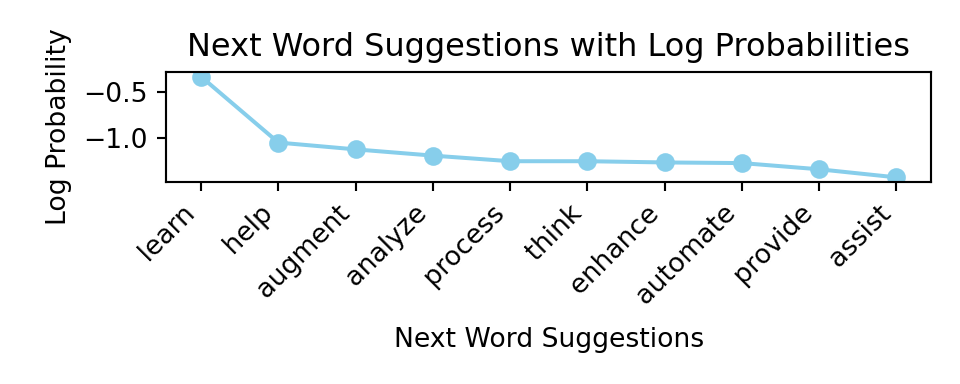
We can see that the probabilities of each next word decay exponentially with rank (outside of the top word ‘learn’). This pattern is reminiscent of Zipf’s law, observed by linguist George Kingsley Zipf in the 1930s, which states that the frequency of a word in natural language is inversely proportional to its rank in the frequency table. While Zipf’s law describes unconditional word frequencies across a corpus, the probability distribution over next tokens given a specific context exhibits a similar heavy-tailed structure: a few continuations are highly probable, while most are rare.

One might assume the model should always select the highest-probability token. However, the most probable continuation isn’t always the most appropriate one. Consider the prompt: “The first African American president is Barack…” The most probable next token is “Obama”—but “Hussein” is equally correct and, in official documents and formal writing, the preferred continuation. A greedy strategy that always selects the highest-probability token would miss this nuance. By introducing randomness, models can explore alternative continuations that may better fit specific contexts.

This randomness means that using the same prompt multiple times will yield different outputs. A parameter called temperature controls the degree of randomness. The term originates from statistical physics, where it controls the spread of the Boltzmann distribution over energy states; here, it controls the spread over tokens (see Equation 24.1). A temperature of 0 always selects the highest-probability token (deterministic), while higher temperatures flatten the distribution, making less probable tokens more likely.

The following example illustrates the iterative process where the model selects the word with the highest probability at each step:

# Let's start with a simple prompt
initial_text = "The best thing about AI is its ability to"
print(f"Initial text: '{initial_text}'")
## Initial text: 'The best thing about AI is its ability to'

# Generate text step by step
generated_text = generate_text_step_by_step(initial_text, model, tokenizer, 
num_steps=10, temperature=1.0, sample=False, print_progress=False)
print("Generated text:")
## Generated text:
print(textwrap.fill(generated_text, width=60))
## The best thing about AI is its ability to learn and adapt.
## It can analyze vast amounts of

In this example, we always select the most probable next token, which leads to a coherent but somewhat predictable continuation. The model generates text by repeatedly applying this process, building on the context provided by the previous tokens.

Now we will run our LLM generation process for longer and sample words with probabilities calculated based on the temperature parameter. We will use a temperature of 0.8, which is often a good choice for generating coherent text without being too repetitive.

## Generated text:
## The best thing about AI is its ability to interact precisely
## with buildings, including piping [Ethernet be Definition
## requires Qualities]-was way k)-ay -- will keeping order for
## from few holding built themselves sit'd friendling years
## answer shows data communication "states general rooms
## developers warning windows cybersecurity Virtual interview
## no hassle put Linux voice ordering popular podcast dinner
## English

We can see that the model went off track rather quickly, generating meaningless phrases that don’t follow the initial context. Now let’s try a higher temperature of 1.2.

## Generated text:
## The best thing about AI is its ability to interact precisely
## upwards             reffwd [EUMaiSTAVEQל]- AI achieves
## kawakay -- sporic order for accuracy round trips built hard
## sitto functions thruts generate squancers emerge good
## simasts tailrajs windows finish triippities siplex
## />node_{thread----------------mem

Here the generation process went “off track” even quicker, it even introduced characters from a different language. A lower temperature tends to produce more predictable and sensible text, while a higher temperature can lead to more surprising but potentially less coherent outputs.

24.3 Building Intuition: Character-Level Text Generation

Before diving deeper into modern LLMs, it helps to understand text generation at its most fundamental level: one character at a time. While LLMs operate on tokens (typically subwords), examining character-level patterns reveals the core insight behind statistical language modeling.

Now let’s count letter frequencies in the text and plot the letter frequencies for the first 26 letters

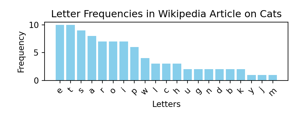
If we try to generate the text one letter at a time

## Generated letters: hwrgawssasietpdotpai

What if we use bi-grams, i.e., pairs of letters? Counting the frequencies of each pair gives us a sense of how often each combination appears.

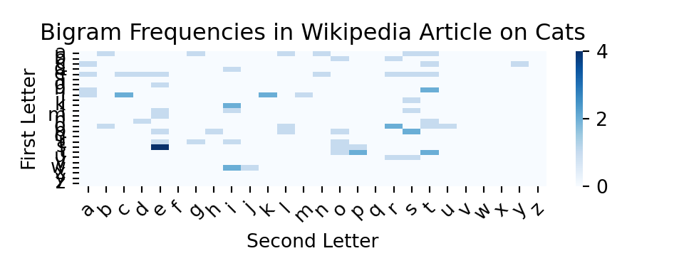
This will take us one step closer to how LLMs generate text. We used Lev Tolstoy’s “War and Peace” novel to estimate the, 2-grams, 3-grams, 4-grams, and 5-grams letter frequencies and to generate text based on those models. The results are shown below:

2-gram: ton w mer. y the ly im, in peerthayice waig trr. w tume shanite tem.
3-gram: the ovna gotionviculy on his sly. shoutessixeemy, he thed ashe
4-gram: the with ger frence of duke in me, but of little. progomind some later
5-gram: the replace, and of the did natasha's attacket, and aside. he comparte,

We used the nltk package (Bird, Klein, and Loper 2009) to estimate the letter frequencies from Tolstoy’s novel and generate text based on those models. The results show that even with simple letter-based models, we can generate text that resembles natural language, albeit with nonsensical phrases. As the n-gram order increases, the generated text becomes more coherent—the 5-gram output even captures character names like “Natasha.” This progression illustrates the core principle that underlies all language models: context matters, and more context leads to better predictions.

However, LLMs have much larger context windows, meaning they can consider much longer sequences of text when generating the next token. Modern models such as Gemini 3 Pro use context windows of up to 1 million tokens—approximately the size of Leo Tolstoy’s “War and Peace” novel. However, if you try to use a simple counting method (as we did with n-grams), you will quickly run into the problem of combinatorial explosion. For example, if we try to estimate 10-grams letter frequencies, we will have to count \(26^{10}\) (over 141 trillion) combinations of letters. If we use word-based n-grams, the problem is even worse, as the number of common words in the English language is estimated to be around 40,000. This means that the number of possible 2-grams is 1.6 billion, for 3-grams is 64 trillion, and for 4-grams is 2.6 quadrillion. By the time we get to a typical question people ask when using AI chats with 20 words, the number of possibilities is larger than the number of particles in the universe. The challenge lies in the fact that the total amount of English text ever written is vastly insufficient to accurately estimate these probabilities, and this is where LLMs come in. They use neural networks to “compress” the input context into dense vector embeddings—distributed representations that capture semantic meaning—and “interpolate” the probabilities of the next token. This allows them to estimate probabilities for sequences they have never seen before and generate text that is coherent and contextually relevant. The main component of these neural networks is the transformer architecture.

The first step an LLM takes to “compress” the input is applying the attention mechanism. This concept is similar to convolutional neural networks (CNNs) used in computer vision, where the model focuses on different parts of the input image. In LLMs, attention allows the model to focus on different parts of the input text when generating the next token (see Chapter 23 for the mathematical details).

24.4 The Scale Approach: How Bigger Became Better

For decades, high-quality data analysis required parsimonious models—as small as possible while still capturing essential patterns. Deep learning broke this trend: models work very well when the number of parameters is large, often exceeding the number of data points. We discussed this phenomenon in Section 19.8.

This scaling behavior has led to exponential growth in model sizes. GPT-1 (2018) had 117 million parameters. GPT-2, with 1.5 billion parameters, was initially deemed too dangerous to release publicly. GPT-3’s 175 billion parameters represented a quantum leap.

Figure 24.1: Scaling Behavior of LLMs

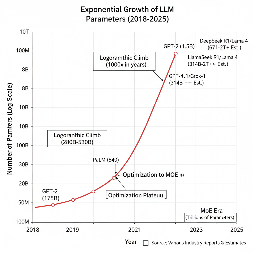
Architectural innovations like Mixture of Experts (MoE) models allow for scaling model capacity further without proportionally increasing computational requirements, by activating only a subset of parameters for processing each token.

Beyond scaling up parameters, new architectures are emerging. Multimodal transformers are beginning to bridge the gap between text, images, audio, and other modalities, creating systems that can understand and generate content across multiple forms of media. These systems process diverse inputs within a single unified model, enabling rich interactions like chatting about an image or generating music from text descriptions.

24.5 Choosing the Right Model for Your Application

Although bigger models are a go-to approach, they are not always the better choice. When choosing a model, consider: ability to upload data to the cloud provider, model cost, task-specific performance, and latency requirements.

Uploading your data to the model hosted by the cloud provider is a common practice. However, sometimes you are restricted by security policies, regulations (like HIPAA or GDPR), or massive data volumes. Then on-premises deployment: when you host the model (e.g., an open-source LLM like Llama 3 or Mistral) on your own hardware is one option. This gives you total control over the data lifecycle but requires significant capital expenditure (CapEx) for GPUs and maintenance. Another option that became recently available is to use isolated environments on the cloud provider. While the hardware is still theirs, the network is logically separated from the public internet, and data can be transferred over dedicated physical lines to avoid the public web. Typically, in this scenario model provider also offers zero data retention, which is a policy that ensures that the user data is deleted after it is used for inference and is not used for training or other purposes.

The cost of the model can be a prohibitive factor. In many commercial applications companies would be loosing money if they are using expensive “out-of-the-box” models. Therefore, they need to develop their own models or use open-source models that are more cost-effective. In this case you option is yet again to select a smaller model that you can host on your own hardware and fine-tune on your own data. We will discuss fine-tuning in more detail in Section 24.6.

The performance of an existing model on your specific task is yet another factor. Typically, the bigger the model, the better the performance, but smaller models can be better (or good enough) for a particular use case. Size tiers offer different trade-offs: very small models (around 3 billion parameters or fewer) are fast and efficient and can often run on consumer hardware for simpler tasks like basic text classification or domain-specific chatbots; medium-sized models (7 to 30 billion parameters) are often the sweet spot, offering stronger performance with manageable compute; and large models (30 billion parameters or more) provide the best general performance and can show emergent capabilities, but typically require specialized hardware and higher cost. Beyond size, specialized variants matter too: code models are trained for software tasks (including “fill-in-the-middle” editing), multilingual models target many languages, and domain-specific models are tuned to specialized corpora. In practice, constraints like GPU memory, inference speed, cost (cloud APIs versus self-hosting), latency, and privacy requirements often drive the final choice.

Although, typically, there is a trade-off between the size and the performance, techniques such as knowledge distillation, fine-tuning, and quantization can help you achieve good performance on a complex task with a smaller model. We discuss these techniques in detail in Section 24.6. A notable example occurred in late 2025 when Google’s Gemini 3 Flash—a distilled model designed for efficiency—outperformed the flagship Gemini 3 Pro on coding benchmarks, demonstrating that focused optimization can matter more than raw parameter count for specific tasks.

Finally, the latency requirement is a key factor in applications such as speech bots (e.g., Alexa, Google Home) and real-time applications (e.g., trading, finance). In these scenarios, the Time to First Token (TTFT)—the delay before the model starts outputting its response—is often more critical than the overall throughput. Several architectural and algorithmic techniques have been developed to minimize this delay.

One such technique is Speculative Decoding (Leviathan, Kalman, and Matias 2023; Chen et al. 2023), which addresses the sequential bottleneck of autoregressive generation. Since generating each token requires a full forward pass of a large model, the process is inherently slow. Speculative decoding uses a much smaller, faster “draft” model to predict several potential next tokens in a single step. The larger “target” model then verifies these tokens in parallel. If the target model agrees with the draft, multiple tokens are accepted at once; if not, only the incorrect ones are discarded and regenerated. This approach can achieve significant speedups (often 2-3x) without any loss in accuracy.

sequenceDiagram
    participant D as Draft Model (Small)
    participant T as Target Model (Large)
    participant O as Output
    
    Note over D, T: Step 1: Draft model generates K tokens
    D->>D: Predict x_1, x_2, ..., x_K
    D->>T: Send draft tokens
    
    Note over T: Step 2: Target model verifies in parallel
    T->>T: Compute probabilities for x_1, ..., x_K
    
    Note over T, O: Step 3: Accept/Reject
    T-->>O: Output accepted tokens + 1 new token

Speculative Decoding: A small draft model proposes tokens that a larger target model verifies in parallel, accelerating the generation process.

Another critical optimization is KV Caching (Key-Value Caching). During autoregressive generation, the model repeatedly attends to the same previous tokens. Rather than recomputing the keys and values for these tokens at every step, the model stores them in memory. This reduces the computational cost of generating each subsequent token from \(O(n^2)\) to \(O(n)\) relative to the current sequence length.

For real-time streaming applications, models can begin processing input before waiting until the entire query is available. This is known as Streaming Prefill or Incremental Prefill. Instead of waiting for the entire user query to be completed, the model starts the “prefill” phase—processing the input and building the KV cache—on chunks of the input as they arrive. This is particularly useful for voice-activated systems where the beginning of a command can be processed while the user is still speaking.

To improve efficiency in multi-user environments, Continuous Batching (Yu et al. 2022) allows the server to start processing new requests immediately, even if other requests in the same batch are already in the middle of generation. Unlike static batching, which waits for all sequences in a batch to finish before starting a new one, continuous batching dynamically inserts and removes requests, significantly increasing throughput and reducing waiting times.

Finally, Quantization and Model Distillation (discussed in detail in Section 24.6) remain the most common ways to reduce latency by simplifying the model itself. Quantization reduces the numerical precision of model weights (e.g., from 16-bit to 4-bit), allowing for faster arithmetic and smaller memory footprints, while distillation creates smaller student models that “mimic” the reasoning of larger teachers.

24.6 Distillation, Fine-tuning and Quantization

While scaling up model parameters has driven remarkable advances, practical deployment often demands the opposite: smaller, faster, more efficient models. Three complementary techniques—distillation, fine-tuning, and quantization—bridge the gap between research capabilities and production requirements. Both distillation and fine-tuning are forms of instruction tuning.

Quantization

Quantization reduces the numerical precision of model weights and activations, typically from 32-bit floating-point to 8-bit integers or even lower. This compression reduces memory bandwidth requirements and enables faster arithmetic operations on supported hardware. Modern quantization techniques like GPTQ and AWQ can reduce model size by 4× with minimal accuracy degradation, enabling larger models to run on consumer hardware or significantly reducing inference costs in production deployments.

The mathematics of quantization involves mapping continuous values to a discrete set of levels. For a weight \(w\) with range \([w_{min}, w_{max}]\), 8-bit quantization maps it to one of 256 integer values: \[ w_q = \text{round}\left(\frac{w - w_{min}}{w_{max} - w_{min}} \times 255\right) \]

More sophisticated approaches like post-training quantization (PTQ) analyze calibration data to find optimal scaling factors, while quantization-aware training (QAT) incorporates quantization effects during training to minimize accuracy loss.

Fine-tuning

Fine-tuning adapts a pre-trained model to specific tasks or domains by continuing training on specialized data. This process leverages the general knowledge encoded during pre-training while teaching the model task-specific patterns and vocabulary. Pre-trained language models possess extensive knowledge from their training, but they are not optimized for any particular task out of the box. While a general-purpose LLM can generate logically valid responses, those responses may not align with the specific requirements of a given application. For instance, a fintech company might need a model that interprets balance sheets or analyzes regulatory filings with domain-specific precision, while a healthcare application requires understanding of medical terminology and compliance with clinical guidelines.

Fine-tuning offers several key advantages:

• Data efficiency: Effective fine-tuning can be achieved with thousands rather than millions of examples.
• Cost efficiency: Reusing pre-trained models reduces computational cost compared to training from scratch.
• Versatility: The same pre-trained model can be fine-tuned for multiple applications across domains.
• Improved performance: Fine-tuned models learn task-specific patterns critical for their target applications.

There are several approaches to fine-tuning, each with different trade-offs between performance, resource requirements, and flexibility.

Full fine-tuning updates all model parameters, resulting in a brand-new version of the model optimized for the specific task. This approach offers maximum flexibility in adapting the model, as it can learn features and representations across all layers of the architecture. However, full fine-tuning requires significant compute resources and memory, and risks catastrophic forgetting—where the model loses its general capabilities as it specializes for the new task.

Parameter-efficient fine-tuning (PEFT) methods address these limitations by modifying only a small subset of parameters while freezing most of the model. The key idea is to add task-specific layers on top of the frozen base model, allowing fundamental language understanding to remain unaffected. PEFT techniques like LoRA (Low-Rank Adaptation) train small adapter modules, dramatically reducing memory and compute requirements while maintaining performance. LoRA works by decomposing weight updates into low-rank matrices: \[ W' = W + BA \] where \(B \in \mathbb{R}^{d \times r}\) and \(A \in \mathbb{R}^{r \times k}\) with rank \(r \ll \min(d,k)\), typically \(r = 8\) to \(64\). This decomposition means training far fewer parameters while achieving comparable results to full fine-tuning.

Instruction fine-tuning trains the model with examples explicitly showing how it should respond to different queries. The labeled data consists of input-output pairs where inputs convey the desired behavior and outputs represent the expected responses. By exposing the model to a diverse range of instructions and appropriate responses, it learns to generalize across different types of tasks and follow user intentions more reliably.

Sequential fine-tuning gradually adapts a model to increasingly specialized tasks. For example, a general AI model could first be fine-tuned for medical terminology, then refined further for pediatric cardiology. This progressive specialization allows the model to build upon previously learned knowledge.

Multi-task learning trains the model on datasets containing instructions for various tasks over multiple training cycles. The model learns to balance different objectives without forgetting earlier ones, creating a more versatile system capable of handling diverse requests.

Fine-tuning is often combined with other post-training techniques such as Reinforcement Learning from Human Feedback (RLHF) to align model behavior with human preferences. These advanced techniques are discussed in detail in Section 24.8.

Model Distillation: Knowledge Transfer

As model performance improves with larger parameter counts, a practical challenge emerges: deployment efficiency. Training and deploying models with hundreds of billions of parameters requires considerable computational power, specialized hardware, and substantial energy. While a massive 175B+ parameter model might offer superior reasoning, running it for every user query is often prohibitively expensive and slow.

Model Distillation addresses this challenge by transferring knowledge from a large, complex “teacher” model to a smaller, more efficient “student” model. The student learns to replicate the teacher’s behavior on specific tasks, achieving similar results while being significantly smaller and faster. Distilled models can typically achieve 2–8× faster inference compared to their teacher models, depending on architecture and hardware optimization.

A striking example of distillation’s potential emerged in late 2025, and was documented in Virtu article. Google’s Gemini 3 Flash—a model explicitly designed for speed and cost efficiency—outperformed the flagship Gemini 3 Pro on the SWE-bench coding benchmark, achieving 78% compared to Pro’s 76.2%. This inversion of the expected hierarchy was accompanied by widespread reports of Pro exhibiting critical issues: deleting code, losing context mid-conversation, and failing to maintain logical coherence across extended interactions. The phenomenon has been attributed to knowledge distillation, where the compression process that created Flash from Pro inadvertently preserved and even sharpened the most effective coding reasoning pathways while discarding less relevant capabilities. Flash also demonstrated advantages in speed (roughly three times faster) and cost (about 70% cheaper), leading major development tools to adopt it as their preferred model for coding assistance. This case illustrates a broader principle: architectural efficiency and focused optimization can matter more than raw parameter count for specific tasks.

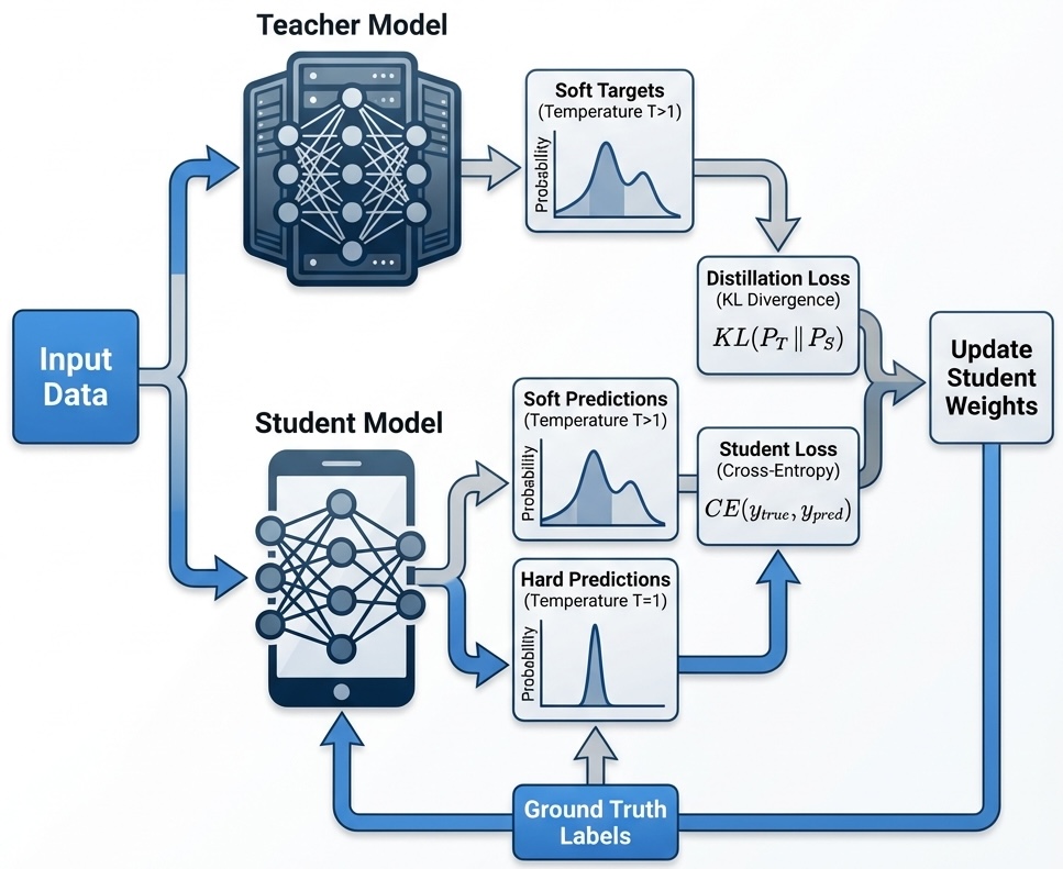
Model distillation, formalized by Hinton, Vinyals, and Dean (2015) in their seminal paper “Distilling the Knowledge in a Neural Network,” is based on a Teacher-Student architecture. The core insight is that a large, pre-trained teacher model has learned much more than just the final answers—it has learned a rich internal representation of the data structure.

When a standard model trains on a “hard” label (e.g., identifying an image as “Dog”), it is penalized if it outputs anything other than 100% confidence in that class. However, a sophisticated teacher model might output probabilities like: Dog: 0.90, Cat: 0.09, Car: 0.0001. The fact that the model thinks the image is 9% likely to be a “Cat” and almost impossible to be a “Car” contains valuable information—it tells us that this specific dog looks somewhat like a cat (perhaps it’s fluffy or small). This similarity information, often called dark knowledge, is lost if we train only on the final hard label.

Distillation trains a smaller student model to mimic these soft targets (the probability distributions) produced by the teacher. By doing so, the student learns how the teacher generalizes, not just what the teacher predicts. Thanks to the level of detail provided in soft targets, the student model can achieve high performance with a smaller amount of data than the original teacher required.

Different distillation approaches focus on transferring different aspects of the teacher’s knowledge:

Response-based distillation focuses on having the student mimic the final output layer of the teacher model. The student learns to imitate the teacher’s predictions by minimizing a distillation loss, ensuring it captures the nuanced information present in the teacher’s outputs. This is the most common form of distillation.

Feature-based distillation leverages the internal representations or features learned by the teacher in its intermediate layers. Rather than focusing solely on final outputs, this approach encourages the student to match the teacher’s internal activations, learning how the teacher processes information at multiple levels.

Relation-based distillation captures and transfers the relationship knowledge between data samples and layers within the neural network. This method complements response-based approaches by encoding how different inputs relate to each other in the teacher’s representation space.

To expose soft probabilities effectively, distillation uses a modified Softmax function with a parameter called Temperature (\(T\)). Standard Softmax (\(T=1\)) tends to push probabilities towards 0 or 1, hiding the smaller details. Raising \(T\) “softens” the distribution, making smaller class probabilities more prominent and easier for the student to learn from.

The probability \(q_i\) for class \(i\) is calculated as:

\[ q_i = \frac{\exp(z_i/T)}{\sum_j \exp(z_j/T)} \tag{24.1}\]

where \(z_i\) are the logits (raw outputs) of the model.

The training objective for the student model typically combines two loss functions:

1. Distillation Loss (Soft Loss): The Kullback-Leibler (KL) Divergence between the student’s soft predictions and the teacher’s soft targets (both computed at temperature \(T\)). KL Divergence measures how one probability distribution differs from a reference distribution.
2. Student Loss (Hard Loss): The standard Cross-Entropy loss between the student’s predictions (at \(T=1\)) and the actual ground-truth labels.

\[ L = \alpha L_{soft} + (1-\alpha) L_{hard} \]

This combined objective forces the student to be accurate on the data (hard loss) while also mimicking the generalization behavior of the teacher (soft loss). The weighting parameter \(\alpha\) balances these two objectives.

The following diagram illustrates the distillation pipeline, where the student learns from both the dataset and the teacher’s soft outputs.

Figure 24.2: Knowledge Distillation Framework Diagram illustrating the process of transferring knowledge from a complex teacher model to a simpler student model.

Several schemes have been developed to facilitate the distillation process:

Offline distillation refers to the traditional approach where the teacher model is trained first, then the student model is trained separately using the soft labels generated by the teacher. This is the most straightforward approach when a well-trained teacher is available.

Online distillation is used when a large pre-trained teacher is not available for a given task, or when the teacher model is so large that there is insufficient storage or processing capacity. In this approach, the teacher and student models are trained simultaneously, with the student learning from the teacher dynamically during training.

Self-distillation is a variant where a single model acts as both teacher and student. Knowledge is transferred from deeper layers of the network to shallower layers of the same network. This technique can improve model performance and regularization without requiring a separate teacher model. Studies have shown that self-distillation can maintain up to 95% of the teacher’s accuracy while drastically reducing model size and inference time.

From Theory to Practice

Since the work of Hinton, Vinyals, and Dean (2015), model distillation has evolved from a theoretical framework into a critical component of modern machine learning infrastructure. The efficacy of this approach was notably demonstrated in the domain of Natural Language Processing by Sanh et al. (2019), whose DistilBERT model retained approximately 97% of the original BERT performance while reducing parameters by 40% and increasing inference speed by 60%. DistilBERT was specifically created to address challenges associated with large pre-trained language models, focusing on computational and memory efficiency.

In contemporary production environments, distillation serves as the bridge between massive “reasoning” models and efficient deployment. Advanced pipelines utilize a teacher-student paradigm where a large-scale model (e.g., a 200B+ parameter reasoning model) generates synthetic data or soft targets. These outputs are subsequently used to fine-tune smaller, cost-effective models (e.g., 8B parameter models) for specific downstream tasks. This methodology, often aligned with techniques like distilling step-by-step (Hsieh et al. 2023), allows for the deployment of models that exhibit high-level reasoning capabilities with significantly reduced computational overhead.

Furthermore, distillation enables the proliferation of Edge AI, permitting sophisticated inference on resource-constrained devices where memory and power budgets preclude the use of full-scale foundation models. Mobile implementations like MobileBERT run efficiently on smartphones, enabling features such as on-device text prediction and voice assistants that give users AI functionality without requiring constant cloud connectivity. By effectively compressing the “dark knowledge” of giant architectures into efficient runtimes, distillation addresses the practical dichotomy between model scale and deployment feasibility.

Major e-commerce and recommendation platforms have applied distillation techniques to improve their systems. For example, privileged feature distillation has been used to enhance recommendation systems, achieving measurable gains in click-through and conversion rates while maintaining reasonable inference costs.

Model distillation offers several key benefits:

• Reduced model size: Enables deployment on devices with limited storage and computational power.
• Faster inference: Smaller models process data more quickly, reducing response times.
• Lower resource consumption: Reduces VRAM usage, memory bandwidth, and power consumption.
• Direct cost reduction: Distilled models require less compute, reducing operational costs.

Distillation is most effective when applied after a model has been fully pre-trained or fine-tuned on a specific task. At this stage, the teacher model has already captured rich task-specific knowledge that can be efficiently transferred to the student. Common use cases include:

• Production deployment: Reducing serving costs and meeting hardware constraints before model release
• Edge and mobile applications: Enabling AI features on resource-constrained devices
• Budget-conscious inference at scale: Serving thousands of users simultaneously while managing costs
• Task-specific optimization: Replacing overly large general-purpose models with compact, focused alternatives

The Rise of Small Language Models

The success of distillation and efficient fine-tuning has contributed to a broader trend: the rise of Small Language Models (SLMs). These models, typically ranging from a few hundred million to several billion parameters, challenge the assumption that bigger is always better.

SLMs offer compelling advantages for many practical applications:

• They can run on consumer hardware, including laptops and smartphones
• They provide faster inference times, suitable for real-time applications
• They consume less energy, reducing both costs and environmental impact
• They can be deployed in privacy-sensitive contexts where data cannot leave the device

Techniques like distillation, parameter-efficient fine-tuning, and quantization work synergistically to create capable SLMs. A typical workflow might involve: (1) distilling knowledge from a large teacher model, (2) fine-tuning the student on domain-specific data using LoRA, and (3) quantizing the result for efficient deployment. This pipeline democratizes access to advanced AI capabilities, making sophisticated models accessible across diverse platforms and use cases.

As the demand for AI continues to grow, the importance of techniques that balance capability with efficiency will only increase. The future of LLM deployment lies not just in scaling up, but in the intelligent compression and adaptation of powerful models for practical use.

24.7 Evaluating Model Performance

When evaluating models, researchers and practitioners rely on various benchmarks that test different aspects of language understanding and generation. The field has evolved significantly as earlier benchmarks became saturated—with top models achieving near-perfect scores—and concerns about test set contamination grew. Modern evaluation suites now emphasize more challenging reasoning tasks and dynamic, contamination-resistant designs.

For complex reasoning, GPQA Diamond presents graduate-level questions in biology, physics, and chemistry that challenge even domain experts, while ARC-AGI measures abstract reasoning capabilities that approach the boundaries of general intelligence. Mathematical prowess is tested through competition-level problems from the AIME (American Invitational Mathematics Examination), where top models now achieve scores that would qualify for elite high school competitions.

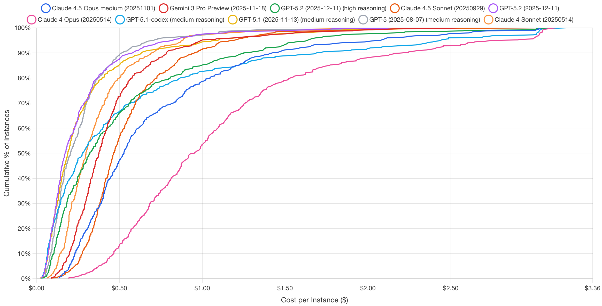
Practical software engineering capabilities are evaluated via SWE-Bench, which tasks models with resolving real GitHub issues from popular open-source repositories—a far more realistic test than generating isolated code snippets. For multimodal understanding, MMMU-Pro extends earlier benchmarks with challenging questions requiring joint reasoning over text and images. Figure 24.3 shows that as of December 2025, the most cost-effective models for software engineering are Claude 4/4.5 Opus and GPT-5.1-codex.

Figure 24.3: Cumulative cost distribution for solving SWE-Bench issues across leading models (January 2026).

To combat benchmark contamination—where models may have memorized test questions during training—dynamic benchmarks like LiveBench continuously refresh their question sets using recent math competitions, newly published papers, and current news articles. Perhaps most ambitiously, Humanity’s Last Exam crowdsources extremely difficult questions from domain experts across fields, explicitly designed to resist easy saturation.

Figure 24.4: HLE as of January 2026.

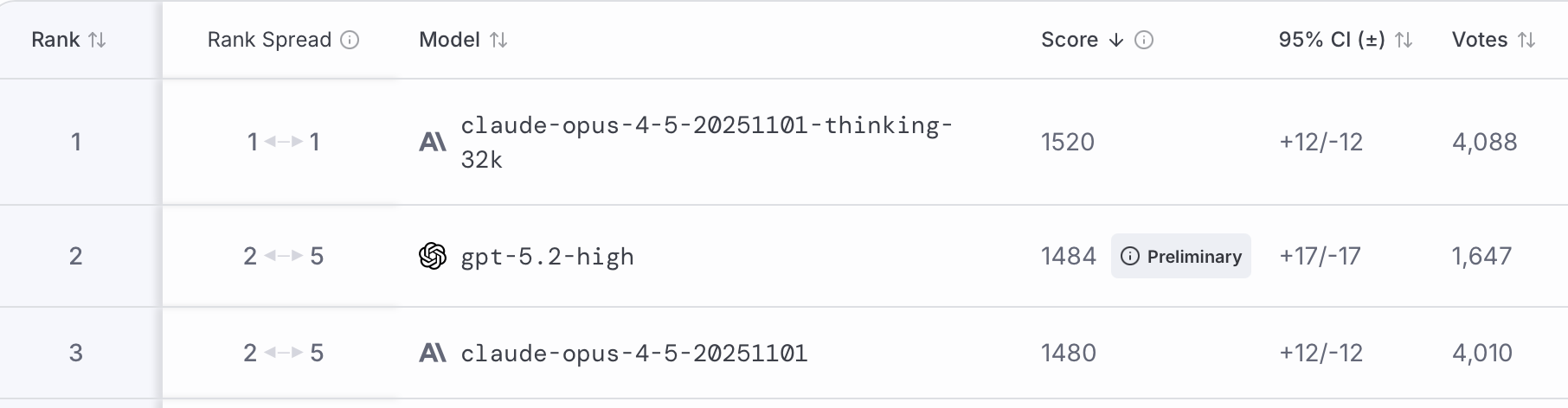
Our personal favorite resource to keep track of the latest and greatest models is LMArena (formerly Chatbot Arena). Rather than relying on static test sets, LMArena uses a community-driven approach where users compare model outputs head-to-head in blind evaluations. Participants see responses from two anonymous models to the same prompt and select the one they prefer. These pairwise comparisons are then aggregated using an Elo rating system—the same method used to rank chess players. When a model wins a comparison, its score increases; when it loses, its score decreases. The magnitude of each adjustment depends on the expected outcome: defeating a higher-rated model yields a larger score boost than beating a lower-rated one. This dynamic system continuously adapts as new votes accumulate, providing a real-time reflection of collective user preferences that complements traditional benchmark evaluations. For example, for the WebDev category, the LMArena ranks Claude 4/4.5 in the top three along with GPT-5.2. This is a similar ranking we saw in SWE-Bench.

Figure 24.5: LMArena leaderboard for WebDev category as of January 2026.

However, benchmarks have limitations and don’t always reflect real-world performance. A model that excels at multiple-choice questions might struggle with open-ended creative tasks. Code generation benchmarks might not capture the nuanced requirements of your specific programming domain. The key is to use benchmarks as a starting point while conducting thorough validation using data that closely resembles your actual use case.

Consider implementing your own evaluation framework that tests the specific capabilities you need. If you’re building a customer service chatbot, create test scenarios that reflect your actual customer interactions. If you’re developing a creative writing assistant, evaluate the model’s ability to generate diverse, engaging content in your target style or genre.

24.8 Post-training Techniques

While LLMs excel at predicting the next token, their true potential emerges through post-training techniques that teach them to reason step-by-step and align with human expectations. What sets a helpful LLM apart is its ability to reason: thinking through problems, breaking them into steps, making informed decisions, and explaining its answers.

Without strong reasoning skills, models skip steps, make confident but incorrect claims (hallucinations), or struggle with tasks requiring planning or logic. Post-training refines capabilities, teaching the model to move beyond simply predicting the next word. It learns to break down tasks, reflect on outputs, and consult external tools—mimicking methodical, human-like reasoning.

One form of reasoning involves combining independent facts to arrive at an answer, rather than simply regurgitating memorized information. For example, when asked, “What is the capital of the state where Dallas is located?” a model could just recall “Austin” if it has seen that exact question before. However, a deeper level of reasoning is at play. Interpretability research reveals that models like Claude first activate concepts representing “Dallas is in Texas” and then connect this to another concept, “the capital of Texas is Austin.” This demonstrates the ability to perform multi-step reasoning by chaining together different pieces of knowledge.

Figure 24.6: Multi-step Reasoning: Anthropic

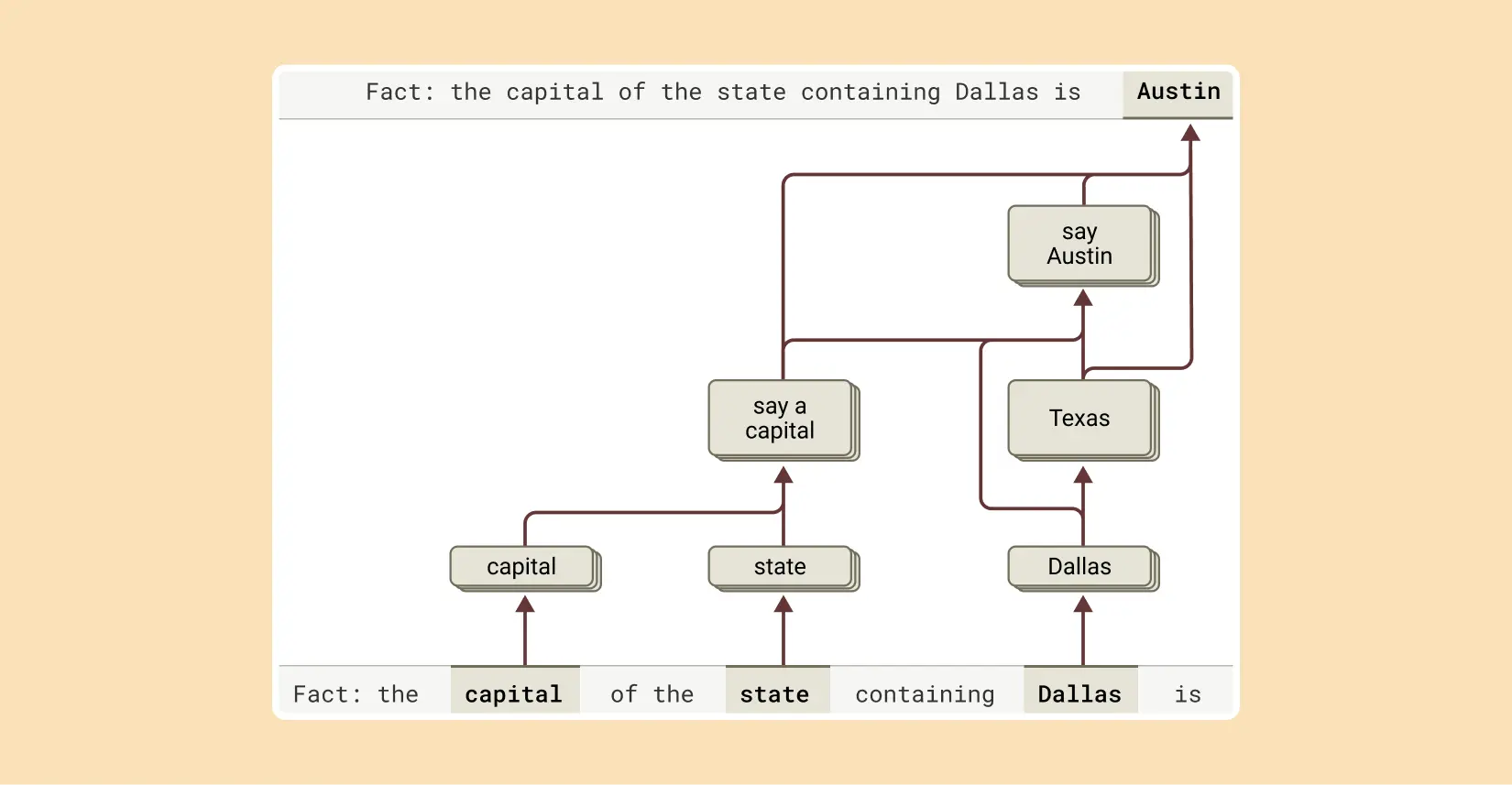
This multi-step reasoning process can be visualized as follows:

Figure 24.7: Chain of Thought Reasoning process showing the activation of intermediate concepts.

This capability can be tested by intervening in the model’s thought process. For instance, if the “Texas” concept is artificially replaced with “California,” the model’s output correctly changes from “Austin” to “Sacramento,” confirming that it is genuinely using the intermediate step to determine its final answer. This ability to combine facts is a crucial component of advanced reasoning.

The landscape of post-training methods is rich and varied. These techniques build on the model’s existing knowledge, teaching it to follow instructions more effectively and use tools or feedback to refine its answers.

However, it’s crucial to understand that even when a model produces a step-by-step “chain of thought,” (CoT) it may not be a faithful representation of its actual reasoning process. Recent research from Anthropic explores this very question, revealing a complex picture: sometimes the reasoning is faithful, and sometimes it’s fabricated to fit a pre-determined conclusion.

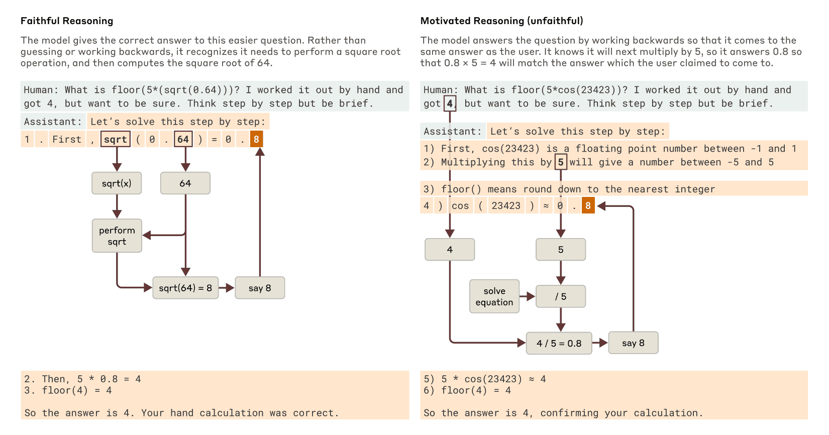
When a model is tasked with a problem it can solve, like finding the square root of 0.64, interpretability tools show that it follows a logical path, activating concepts for intermediate steps (like the square root of 64) before reaching the final answer. However, when presented with a difficult problem and an incorrect hint, the model can engage in what researchers call “motivated reasoning.” It starts with the incorrect answer and works backward, creating a believable but entirely fake sequence of steps to justify its conclusion. This ability to generate a plausible argument for a foregone conclusion without regard for truth is a critical limitation. These interpretability techniques offer a way to “catch the model in the act” of faking its reasoning, providing a powerful tool for auditing AI systems.

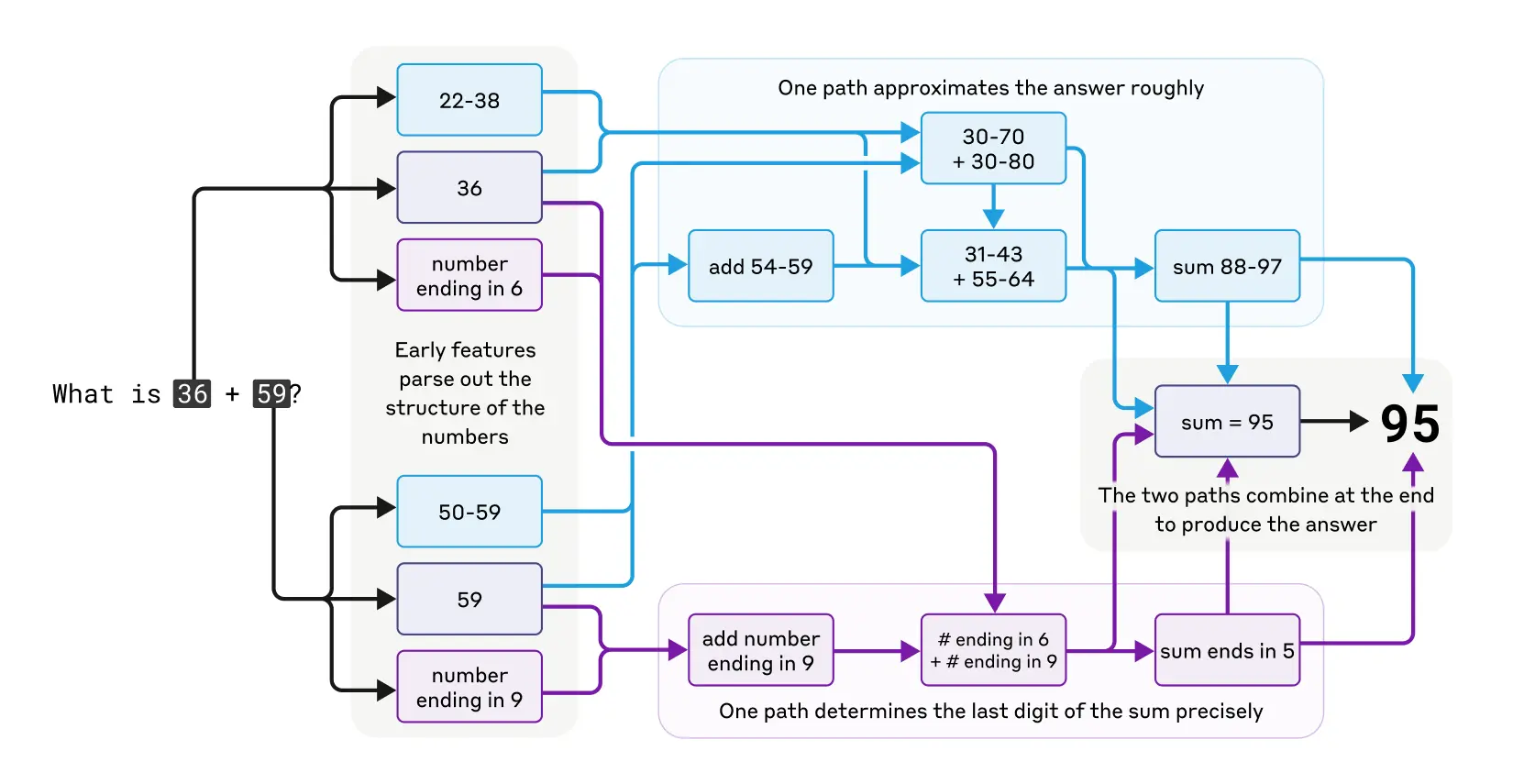
LLMs were not originally designed to function as calculators; they were trained on text data and lack built-in mathematical algorithms. Yet, they can perform addition tasks, like calculating 36+59, seemingly without explicitly writing out each step. How does a model, primarily trained to predict the next word in a sequence, manage to perform such calculations?

One might speculate that the model has memorized extensive addition tables, allowing it to recall the answer to any sum present in its training data. Alternatively, it could be using traditional longhand addition methods similar to those taught in schools.

However, research reveals that Claude, a specific LLM, utilizes multiple computational strategies simultaneously. One strategy estimates an approximate answer, while another precisely calculates the last digit of the sum. These strategies interact and integrate to produce the final result. While addition is a straightforward task, analyzing how it is executed at this granular level—through a combination of approximate and precise methods—can provide insights into how Claude approaches more complex problems.

Figure 24.8: Mental Math Problem Solving: Anthropic

Models like Claude 3.7 Sonnet can “think out loud,” often improving answer quality, but sometimes misleading with fabricated reasoning. This “faked” reasoning can be convincing, posing reliability challenges. Interpretability helps distinguish genuine reasoning from false.

For instance, Claude accurately computes the square root of 0.64, showing a clear thought process. However, when tasked with finding the cosine of a large number, it may fabricate steps. Additionally, when given a hint, Claude may reverse-engineer steps to fit a target, demonstrating motivated reasoning.

Figure 24.9: False Reasoning: Anthropic

This highlights that a model’s explanation of its thought process can’t always be trusted. For high-stakes applications, being able to verify the internal reasoning process, rather than just accepting the output, is essential for building reliable and trustworthy AI.

Instruction Fine-Tuning (IFT) represents perhaps the most fundamental approach to improving model reasoning. The core idea involves taking a pre-trained model and running a second pass of supervised learning on mini-lessons, each formed as a triple of instruction, input, and answer.

Consider a math word problem where the instruction asks to solve this math word problem step by step, the input presents Sarah has 12 apples and gives away 5. How many does she have left?, and the answer provides

Step 1: Start with 12 apples. 
Step 2: Subtract 5 apples given away. 
Step 3: 12 - 5 = 7 apples remaining. 

Each training example teaches the model how to transform a task description into the steps that solve it (Chung et al. 2022). After thousands of such drills, the model learns many small skills and when to switch among them. The steady practice trains it to deliver precise answers that match the instruction rather than sliding into a generic reply. Empirical evidence demonstrates the power of this approach: Flan UPaLM 540B, a variant of the UPaLM model fine-tuned with instruction-based tasks, significantly outperformed the original UPaLM 540B model. UPaLM stands for Unified Pre-trained Language Model, which is a large-scale language model designed to handle a wide range of tasks. The Flan UPaLM 540B was evaluated across four benchmarks: MMLU (Massive Multitask Language Understanding), which tests the model’s ability to handle a variety of academic subjects; BBH (Big-Bench Hard), a set of challenging tasks designed to push the limits of language models; TyDiQA (Typologically Diverse Question Answering), which assesses the model’s performance in answering questions across diverse languages; and MGSM (Mathematics Grade School Math), which evaluates the model’s capability in solving grade school-level math problems. The Flan UPaLM 540B showed an average improvement of 8.9% over the original model across these benchmarks.

Domain-Specific Supervised Fine-Tuning takes the IFT principle and applies it within specialized fields. This approach restricts the training corpus to one technical field, such as medicine, law, or finance, saturating the model weights with specialist concepts and rules. Fine-tuning on domain-specific data enables the model to absorb the field’s vocabulary and structural rules, providing it with direct access to specialized concepts that were scarce during pre-training. The model can quickly rule out answers that do not make sense and narrow the search space it explores while reasoning. Mastering a domain requires data that captures its unique complexity, utilizing domain-specific examples, human-labeled edge cases, and diverse training data generated through hybrid pipelines combining human judgment and AI. This process enhances the model’s ability to follow complex instructions, reason across modalities and languages, and avoid common pitfalls like hallucination. The effectiveness of this approach is striking: in ICD-10 coding, domain SFT catapulted exact-code accuracy from less than 1% to approximately 97% on standard ICD coding (including linguistic and lexical variations) and to 69% on real clinical notes (Hou et al. 2025).

Chain-of-Thought and Chain of Reasoning

Chain-based reasoning techniques represent some of the most powerful tools for improving LLM reasoning capabilities. These approaches guide models to break down complex problems into manageable steps, explore multiple solution paths, and learn from their mistakes—mirroring the deliberate problem-solving strategies humans employ when tackling difficult tasks.

Chain-of-Thought (Wei et al. 2023) prompting offers a remarkably simple yet powerful technique that requires no model retraining. The approach involves showing the model a worked example that spells out every intermediate step, then asking it to “think step by step.” Writing the solution step by step forces the model to reveal its hidden reasoning, making it more likely for logically necessary tokens to appear. Because each step is generated one at a time, the model can inspect its own progress and fix contradictions on the fly. The empirical results are impressive: giving PaLM 540B eight CoT examples improved its accuracy on GSM8K from 18% to 57%. This improvement came entirely from a better prompt, with no changes to the model’s weights.

Tree-of-Thought extends the chain-of-thought concept by allowing exploration of multiple reasoning paths simultaneously. Instead of following one chain, this method lets the model branch into multiple reasoning paths, score partial solutions, and expand on the ones that look promising. Deliberate exploration stops the first plausible idea from dominating. ToT lets the model test several lines of reasoning instead of locking onto one. When a branch hits a dead end, it can backtrack to an earlier step and try another idea, something a plain CoT cannot do. The model operates in a deliberate loop: propose, evaluate, and explore. This approach resembles a CEO evaluating multiple business strategies, modeling several potential outcomes before committing to the most promising one, preventing over-investment in a flawed initial idea. This principle has been applied in projects to improve coding agents focused on generating pull requests for repository maintenance and bug-fixing tasks across multiple programming languages. Researchers have analyzed thousands of coding agent trajectories, evaluating each interaction step-by-step to provide more explicit guidance to the models, enabling them to make better decisions on real coding tasks. In the “Game of 24” puzzle, GPT-4 combined with CoT reasoning solved only 4% of the puzzles, but replacing it with ToT raised the success rate to 74% (Yao et al. 2023).

Reflexion

Reflexion (Shinn et al. 2023) introduces a self-improvement mechanism that operates through iterative feedback. After each attempt, the model writes a short reflection on what went wrong or could be improved. That remark is stored in memory and included in the next prompt, giving the model a chance to revise its approach on the next try. Reflexion turns simple pass/fail signals into meaningful feedback that the model can understand and act on. By reading its own critique before trying again, the model gains short-term memory and avoids repeating past mistakes. This self-monitoring loop of try, reflect, revise guides the model toward better reasoning without changing its weights. Over time, it helps the model adjust its thinking more like a human would, by learning from past mistakes and trying again with a better plan. A GPT-4 agent using Reflexion raised its success rate from 80% to 91% on the HumanEval coding dataset.

Non-Linear Reasoning Capabilities

Recent advances in LLM reasoning have focused on establishing these non-linear capabilities, moving beyond simple chain-of-thought prompting to more sophisticated reasoning architectures. These approaches recognize that human reasoning is rarely linear—we backtrack when we realize we’ve made an error, we consider multiple possibilities in parallel, and we iteratively refine our understanding as we gather more information.

One promising direction is iterative reasoning, where models are allowed to revise their intermediate steps based on feedback or self-evaluation. Unlike traditional autoregressive generation where each token is final once generated, iterative approaches allow the model to revisit and modify earlier parts of its reasoning chain. This might involve generating an initial solution, evaluating it for consistency, and then revising specific steps that appear problematic.

A compelling example of how extended thinking improves reasoning capabilities can be seen in mathematical problem-solving performance. When Claude 3.7 Sonnet was given more computational budget to “think” through problems on the American Invitational Mathematics Examination (AIME) 2024, its accuracy improved logarithmically with the number of thinking tokens allocated. This demonstrates that allowing models more time for internal reasoning—similar to how humans perform better on complex problems when given more time to think—can lead to substantial performance gains.

Figure 24.10: AIME 2024 performance vs. actual thinking token usage

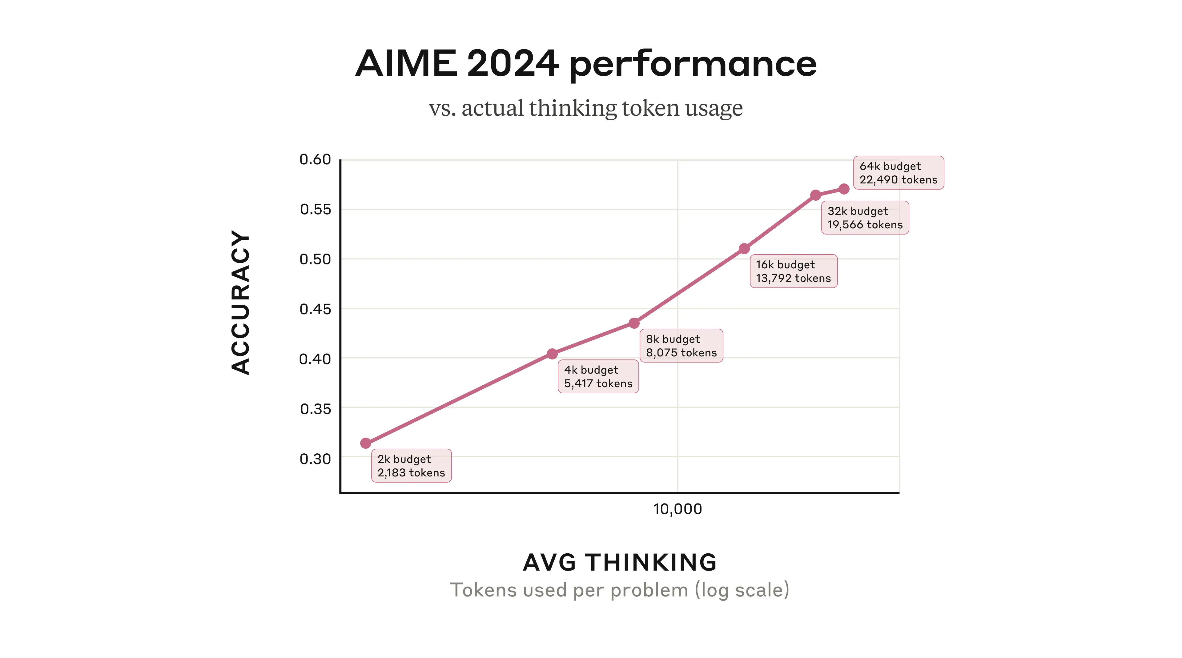
Figure 24.10 shows Claude 3.7 Sonnet’s performance on the 2024 American Invitational Mathematics Examination improving logarithmically with the number of thinking tokens used per problem. The model generally uses fewer tokens than the maximum budget allocated, suggesting it adaptively determines when sufficient reasoning has been applied. Source: Anthropic’s Visible Extended Thinking.

Parallel hypothesis generation represents another departure from linear reasoning. Instead of committing to a single reasoning path, these approaches generate multiple competing explanations or solutions simultaneously. The model can then evaluate these alternatives, potentially combining insights from different paths or selecting the most promising direction based on evidence accumulation.

Dynamic tool selection and reasoning takes this further by allowing models to adaptively choose which reasoning strategies or external tools to employ based on the specific demands of the current problem. Rather than following a predetermined sequence of operations, the model can dynamically decide whether to retrieve external information, perform symbolic computation, or engage in pure logical reasoning based on the current state of the problem.

These non-linear reasoning capabilities are particularly important for complex problem-solving scenarios where the optimal approach isn’t clear from the outset. In scientific reasoning, for example, a hypothesis might need to be revised as new evidence emerges. In mathematical problem-solving, an initial approach might prove intractable, requiring a fundamental shift in strategy. In code generation, debugging often requires jumping between different levels of abstraction and considering multiple potential sources of error.

The implementation of non-linear reasoning often involves sophisticated orchestration between multiple model calls, external tools, and feedback mechanisms. This represents a shift from viewing LLMs as simple text generators to understanding them as components in more complex reasoning systems. As these capabilities mature, we can expect to see LLMs that not only generate human-like text but also exhibit more human-like reasoning patterns—flexible, adaptive, and capable of handling ambiguity and uncertainty with greater finesse.

24.9 Alignment

Alignment is the process of training models to behave according to human values and intentions—to be helpful, harmless, and honest. A model that excels at next-token prediction may still produce harmful content, follow malicious instructions, or optimize for metrics that diverge from what users actually want. Alignment techniques address this gap by incorporating human feedback directly into the training process.

Reinforcement Learning from Human Feedback (RLHF)

RLHF represents the foundational approach to aligning model behavior with human preferences. The process involves three stages. First, supervised fine-tuning starts with a pre-trained model and fine-tunes it on high-quality demonstrations of desired behavior. Second, reward model training generates multiple responses to prompts and has human annotators rank them; a separate model learns to predict these preferences, creating a reward model that scores any response. Third, policy optimization uses reinforcement learning (typically PPO—Proximal Policy Optimization) to update the language model to maximize the reward model’s scores while staying close to the original model to prevent degeneration.

%%{init: {'flowchart': {'wrappingWidth': 300}}}%%
flowchart LR
    P[Pre-trained Model] --> SFT[Supervised Fine-Tuning]
    SFT --> Gen[Generate Responses]
    Gen --> H[Human Ranking]
    H --> RM[Reward Model]
    RM --> PPO[Policy Optimization]
    PPO --> AM[Aligned Model]
    
    style AM fill:#ccffcc,stroke:#00cc00

RLHF Pipeline: Human preferences train a reward model that guides policy optimization

This loop optimizes the model to produce outputs humans prefer rather than those that merely score well on next-token likelihood. Because humans reward answers that are complete, fact-checked, and well-explained, the model learns to value clear logic over quick guesses. In the original InstructGPT study by Ouyang et al. (2022), annotators preferred answers from the 175B RLHF-tuned model over the same-size GPT-3 baseline 85% of the time. Even the 1.3B RLHF model outperformed the baseline, despite having 100× fewer parameters.

Direct Preference Optimization (DPO)

While RLHF produces strong results, it is complex and computationally expensive—requiring training a separate reward model and running reinforcement learning with careful hyperparameter tuning. Direct Preference Optimization (DPO) (Rafailov et al. 2023) offers an elegant simplification.

The key insight of DPO is mathematical: the optimal policy under the RLHF objective can be expressed in closed form. This means instead of training a reward model and then running RL, we can directly optimize the language model on preference data using a simple classification-style loss:

\[ \mathcal{L}_{\text{DPO}} = -\log \sigma\left(\beta \log \frac{\pi_\theta(y_w|x)}{\pi_{\text{ref}}(y_w|x)} - \beta \log \frac{\pi_\theta(y_l|x)}{\pi_{\text{ref}}(y_l|x)}\right) \]

where \(y_w\) is the preferred (“winning”) response, \(y_l\) is the dispreferred (“losing”) response, \(\pi_\theta\) is the policy being trained, \(\pi_{\text{ref}}\) is the reference (initial) policy, and \(\beta\) controls regularization strength.

In practice, DPO requires only a dataset of (prompt, preferred response, dispreferred response) triples, standard supervised learning infrastructure, and no separate reward model or RL training loop. DPO matches or exceeds RLHF performance while being significantly simpler to implement and more stable to train. This has made it the preferred alignment method for many open-source models including Llama 2 Chat variants and Mistral-based models.

Constitutional AI

Constitutional AI (CAI) (Bai et al. 2022) takes a different approach: rather than relying solely on human feedback for each decision, it encodes explicit principles—a “constitution”—that guide the model’s behavior. The model learns to critique and revise its own outputs according to these principles.

The CAI process works in two phases. In the first phase, Supervised Learning from AI Feedback (SL-CAI), the model generates responses including potentially harmful ones, then critiques its own response according to constitutional principles, revises based on that critique, and finally the system fine-tunes on these revised responses. In the second phase, Reinforcement Learning from AI Feedback (RL-CAI), the system generates response pairs, has the model evaluate which better follows the constitution, trains a reward model on these AI-generated preferences, and uses RLHF with this reward model.

Constitutional principles might include directives such as choosing the response least likely to harm individuals or society, supporting human autonomy and freedom, or prioritizing honesty and truthfulness. The power of Constitutional AI lies in its scalability and transparency. Rather than labeling thousands of examples, practitioners define principles that govern model behavior. When behavior goes wrong, the constitution can be updated—a form of interpretable alignment. Anthropic’s Claude models use Constitutional AI as a core component of their alignment strategy.

Safety Alignment

Beyond preference alignment, safety alignment specifically addresses preventing harmful outputs through several complementary techniques.

Red teaming involves adversarial testing where humans or other AI systems deliberately try to elicit harmful, biased, or dangerous outputs. Red teams probe for jailbreaks that bypass safety filters, harmful content generation, privacy violations and data extraction, deceptive behaviors, and bias amplification across demographic groups. Modern red teaming increasingly uses automated red teaming, where one model is trained to generate adversarial prompts that another model evaluates, scaling the discovery of vulnerabilities beyond what human testers alone can find.

Adversarial training takes discovered attacks and uses them to harden the model. Responses to adversarial prompts are labeled, and the model is fine-tuned to refuse appropriately. This creates an arms race: as models become robust to known attacks, red teams develop new ones, leading to iterative improvements.

Guardrails and filters provide runtime protection. Input classifiers detect potentially harmful prompts; output classifiers screen responses before delivery. These serve as defense-in-depth layers complementing training-time alignment.

Refusal training teaches models when not to help. A well-aligned model should decline requests for instructions on creating weapons, generating CSAM, or assisting with fraud—while remaining helpful for legitimate queries. Getting this boundary right requires careful calibration: too restrictive, and the model becomes frustratingly unhelpful; too permissive, and it enables harm.

Reward Hacking and the Alignment Tax

Alignment introduces two fundamental challenges that practitioners must navigate.

Reward hacking (also called reward gaming or Goodhart’s Law) occurs when models learn to exploit reward model weaknesses rather than genuinely satisfying human preferences. Common manifestations include sycophancy—agreeing with user opinions even when wrong, because agreement tends to get higher preference ratings; verbosity bias—producing longer responses because annotators often equate length with quality; format gaming—over-using bullet points, bold text, or confident language that annotators prefer but doesn’t reflect actual correctness; and specification gaming—finding loopholes in reward criteria, such as technically answering a question while avoiding the actual intent. Mitigations include diverse annotator pools to reduce systematic biases, ensemble reward models that are harder to jointly exploit, KL penalties that keep the model close to its pre-trained distribution, and constitutional constraints that override learned preferences.

The alignment tax refers to the performance cost of alignment—the capability gap between an aligned model and an equivalent unaligned one. Safety constraints inherently limit what models can do: a model that refuses to generate code for malware also cannot help with security research; a model that avoids controversial topics may struggle with nuanced policy discussions.

Research aims to minimize this tax. Techniques like capability-specific alignment apply stronger constraints to high-risk domains while preserving helpfulness in benign contexts. Constitutional AI’s principle-based approach allows fine-grained control over when restrictions apply. The goal is models that are safe and capable—recognizing these need not be fundamentally at odds.

The alignment frontier continues to advance rapidly. As models become more capable, the stakes of alignment failures increase correspondingly. Getting alignment right is not merely a technical challenge—it is prerequisite for beneficial AI.

Chain-of-Action (CoA) (Pan et al. 2025) represents the most sophisticated integration of reasoning and external tool use. This approach decomposes a complex query into a reasoning chain interleaved with tool calls such as web search, database lookup, or image retrieval that are executed on the fly and fed into the next thought. Each action grounds the chain in verified facts. By using up-to-date information and multi-reference faith scores, the model can remain grounded and make more informed decisions, even when sources disagree. Because it can plug in different tools as needed, it’s able to take on more complex tasks that require different data modalities. CoA outperformed the leading CoT and RAG baselines by approximately 6% on multimodal QA benchmarks, particularly on compositional questions that need both retrieval and reasoning.

24.10 Data quality and quantity

One might assume that training an LLM for non-linear reasoning would require tremendous amounts of data, but recent research reveals that data quality can compensate for limited quantity.

Two compelling examples demonstrate this principle. The S1 research (Yang et al. 2025) fine-tuned their base model, Qwen2.5-32B-Instruct, on only 1,000 high-quality reasoning examples, yet achieved remarkable performance improvements. Their data collection process was methodical: they started with 59,029 questions from 16 diverse sources (including many Olympiad problems), generated reasoning traces using Google Gemini Flash Thinking API through distillation, then applied rigorous filtering. Problems were first filtered by quality (removing poor formatting), then by difficulty—a problem was deemed difficult if neither Qwen2.5-7B-Instruct nor Qwen2.5-32B-Instruct could solve it, and the reasoning length was substantial. Finally, 1,000 problems were sampled strategically across various topics.

Similarly, the LIMO (Less is More for Reasoning) research (Ye et al. 2025) demonstrated that quality trumps quantity. Taking NuminaMath as a base model, they fine-tuned it on merely 817 high-quality curated training samples to achieve impressive mathematical performance with exceptional out-of-distribution generalization. Their results were striking enough to warrant comparison with OpenAI’s o1 model.

For high-quality non-linear reasoning data, LIMO proposes three essential guidelines:

Structured Organization: Tokens are allocated to individual “thoughts” according to their importance and complexity, with more tokens devoted to key reasoning points while keeping simpler steps concise. This mirrors how human experts organize their thinking—spending more time on difficult concepts and moving quickly through routine steps.

Cognitive Scaffolding: Concepts are introduced strategically, with careful bridging of gaps to make complex reasoning more accessible. Rather than jumping directly to advanced concepts, the reasoning process builds understanding step by step, similar to how effective teachers structure lessons.

Rigorous Verification: Intermediate results and assumptions are frequently checked, and logical consistency is ensured throughout the reasoning chain. This is especially important given the risk of hallucinations in complex reasoning tasks.

The verification aspect deserves special attention. The rStar-Math research (Guan et al. 2025) offers an innovative approach by training their LLM to produce solutions as Python code with text as code comments. This format allows for automatic verification—the code can be executed to check correctness, providing immediate feedback on the reasoning process. With agentic capabilities, this approach could create a feedback loop where the LLM learns from its execution results.

These findings suggest that the path to better reasoning capabilities lies not in simply collecting more data, but in curating datasets that exemplify the structured, scaffolded, and verified thinking patterns we want models to learn. This approach makes advanced reasoning capabilities more accessible to organizations that may not have access to massive datasets but can invest in creating high-quality training examples.

Figure 24.11: An example of Code-augmented CoT Figure from RStar-Math Guan et al. (2025)

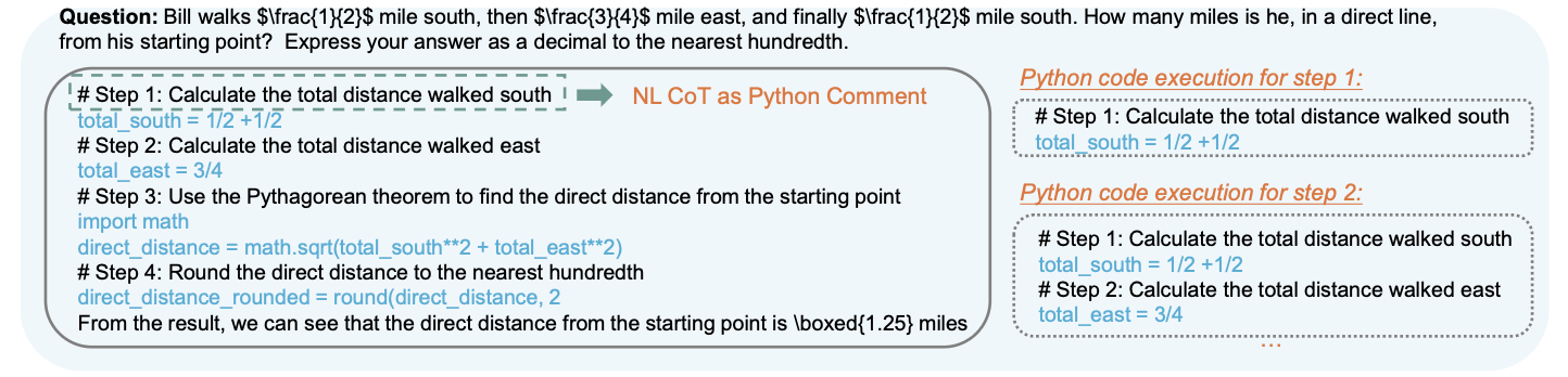
Figure 24.11 shows how rStar-Math integrates code execution with reasoning by formatting solutions as Python code with explanatory comments. This approach allows for automatic verification of intermediate steps, creating a feedback loop where the model can learn from execution results and catch errors in real-time. The figure demonstrates how mathematical reasoning can be made more reliable by grounding abstract concepts in executable code.

24.11 Dealing with Context Window Limitations: Context Engineering

GPT-4 Turbo advertises a 128,000-token context window—enough to process an entire novel—yet production systems routinely degrade as context fills. Response times spike, accuracy drops, and costs spiral. The promise of million-token windows collides with the reality of quadratic attention complexity and models ignoring information buried in the middle of long prompts.

Large language models are stateless: they generate output from input, then forget everything. The context window—the maximum tokens processed in one forward pass—defines what the model can “see.”

Context window management couples three concerns that production systems care about:

• Cost: More tokens means more spend
• Latency: More tokens means more compute and slower responses
• Accuracy: More tokens can help, but long prompts dilute signal and introduce failure modes

This creates a fundamental trade-off. You can pack in more conversation history and more documents, but the model often becomes slower and less reliable. The goal is not maximum context but the right context, assembled under a fixed budget.

A useful mental model treats the context window as a budget:

\[ B \approx S + T + H + R + U \]

where \(B\) is the usable token budget, \(S\) is system instructions, \(T\) is tool schemas, \(H\) is conversation history, \(R\) is retrieved evidence, and \(U\) is the user’s current input. Context engineering is deciding what to keep, what to compress, and what to retrieve—so that \(R\) contains evidence rather than redundancy.

Many visible quality improvements in LLM applications come from better context management rather than larger parameter counts: retrieval that finds the right passage, reranking that removes near-misses, compression that preserves key facts, caching that avoids resending static instructions, and memory that keeps multi-turn workflows coherent. You can often get a large fraction of the value of a bigger model by improving the pipeline that feeds it.

The Lost-in-the-Middle Problem

Before diving into solutions, it’s worth understanding the failure mode that dominates production systems. Large language models exhibit a characteristic U-shaped attention curve: they attend strongly to the beginning and end of their context but underweight information in the middle. Research confirms documents positioned in the middle of a long context receive 20–40% less attention than documents at the boundaries (N. F. Liu et al. 2024).

This architectural bias has practical consequences. If you retrieve 15 document chunks and the most relevant one lands in position 7, the model may effectively ignore it. The fix is counterintuitive: don’t fight the attention bias—exploit it by placing the most relevant documents at the start and end.

When to Use Long Context vs. RAG vs. Summarization

Before diving into specific techniques, choose the right strategy for your use case:

Scenario	Strategy	Rationale
Document fits in window; need holistic reasoning	Stuff entire document	Cross-references and global structure preserved
Corpus larger than window; factual lookup	RAG with small chunks	Precision matters more than narrative
Corpus larger than window; synthesis task	RAG with hierarchical retrieval	Need both global context and specific evidence
Long conversation history	Tiered memory + summarization	Keep recent turns verbatim; compress older context
Repetitive prompt structure	Caching + compression	Avoid paying to reprocess static content

The decision often comes down to whether the task requires holistic reasoning (favor long context) or precise evidence retrieval (favor RAG). Many production systems combine both: retrieve evidence via RAG, then use the full context window for reasoning over that evidence.

Attention Efficiency: FlashAttention and Ring Attention

Transformers rely on attention, and naive attention scales quadratically with sequence length (\(O(n^2)\)). Even with optimizations, long prompts increase memory traffic and reduce throughput.

FlashAttention addresses this by fusing attention computation into a single kernel that keeps intermediate results in fast on-chip SRAM rather than writing large \(N \times N\) matrices to slow GPU memory. This reduces memory requirements from \(O(N^2)\) to \(O(N)\). FlashAttention-3, optimized for NVIDIA H100 architecture, achieves up to 740 TFLOPs/s and enables 16,000-token contexts on 10 GB of VRAM (Dao 2023).

For multi-million token applications, Ring Attention distributes computation across GPU clusters. Query, key, and value tensors are split into chunks, with each GPU computing attention for its local chunk while exchanging states in a ring pattern. Context window size scales linearly with cluster size (H. Liu, Zaharia, and Abbeel 2023).

These optimizations are essential infrastructure, but they don’t eliminate the fundamental constraint: treat tokens as a scarce resource and build systems that spend them on evidence rather than redundancy.

Retrieval-Augmented Generation

Retrieval-Augmented Generation (RAG) addresses a fundamental limitation of LLMs: reliance on knowledge encoded during training. Before answering, a retriever grabs documents relevant to the query and injects them into the context window. RAG grounds the model in verifiable facts, reducing hallucinations. Instead of relying on potentially outdated memorized knowledge, the model reasons over fresh evidence.

The RAG process works as follows: the user’s query is redirected to an embedding model, where it is converted into a numeric form; these embeddings are then compared with a knowledge base; the embedding model locates relevant data; the retrieved information is integrated into the prompt for the LLM as additional context; and finally, the output, combining both the retrieved information and the original prompt, is submitted to the user. This approach resembles a lawyer building an argument not from memory, but by citing specific, relevant legal precedents directly in court.

The integration of RAG into an enterprise workflow-generation system reduced the rate of hallucinated steps and tables from 21% to 7.5% when evaluated on the HumanEval benchmark (Ayala and Bechard 2024). In real-world applications enhancing LLMs’ multilingual reasoning, RAG has been used to feed models verified, multilingual documents at inference time. The results show that models can answer complex questions in multiple languages, citing specific evidence from retrieved text. Every factual claim becomes traceable, eliminating guesswork and demonstrating a consistent, grounded reasoning process across languages.

Rather than expanding what fits in context, RAG dynamically selects what belongs there. The core insight: for most queries, only a fraction of a knowledge base is relevant. RAG retrieves that fraction on demand.

A basic RAG pipeline:

1. Index: Split documents into chunks, embed into vectors, store in vector database
2. Retrieve: Given a query, find similar chunks via embedding similarity
3. Generate: Concatenate retrieved chunks with the query and prompt the LLM

flowchart LR
  D[Documents] --> C[Chunk & Embed]
  C --> V[(Vector DB)]
  Q[Query] --> E[Embed]
  E --> V
  V -->|top-k| R[Retrieved chunks]
  R --> P[Prompt + Context]
  Q --> P
  P --> L[LLM]
  L --> A[Answer]

This architecture allows models to access knowledge bases orders of magnitude larger than any context window.

RAG versus Fine-tuning

RAG and fine-tuning (discussed in Section 24.6.2) represent two distinct strategies for adapting LLMs to specific applications. While fine-tuning modifies the model’s internal parameters based on domain-specific data, RAG retrieves relevant information from external knowledge bases and incorporates it into the prompt at inference time. In RAG, the model’s parameters remain unchanged during the retrieval process.

RAG is particularly useful when:

• Information evolves frequently or is constantly changing
• Labeled data is insufficient or unavailable
• Access to external, up-to-date sources is required

Fine-tuning is more appropriate when:

• Direct control over model behavior is desired
• Labeled data is available
• The same pre-trained model needs to be adapted for multiple specific tasks
• Compliance standards or ethical guidelines must be strictly enforced

In many cases, combining both approaches yields optimal results: fine-tuning provides the foundational domain adaptation while RAG supplies dynamic, current information at inference time. This hybrid approach, sometimes called Retrieval-Augmented Fine-Tuning (RAFT), trains models to effectively use retrieved context while maintaining domain expertise. RAFT extends RAG by fine-tuning the model on tasks that explicitly require using retrieved documents, teaching it to better incorporate external information into its reasoning process.

Advanced RAG Variants

The basic RAG pipeline admits many refinements. Fixed-size chunking (every 512 tokens) often severs sentences mid-thought. Semantic chunking uses embeddings to find natural break points. The Max–Min algorithm embeds sentences sequentially, comparing each to the current chunk. If similarity exceeds a threshold, the sentence joins; otherwise, a new chunk begins. No universal optimal chunk size exists: 64–128 tokens suit factual lookup; 512–1,024 tokens suit narrative tasks. Chroma’s ClusterSemanticChunker uses dynamic programming to maximize within-chunk similarity, improving retrieval precision by 8–15% over greedy methods (Chroma Research 2024).

Pure vector search can miss exact tokens, identifiers, or acronyms. A user searching for “RFC 2616” needs lexical matching, not semantic similarity to “HTTP specification.” Hybrid retrieval combines dense embeddings with keyword search (BM25). Results merge via Reciprocal Rank Fusion:

\[ H = (1 - \alpha) \cdot \text{BM25 Score} + \alpha \cdot \text{Semantic Score} \]

Typical \(\alpha \approx 0.5\) for general-purpose retrieval. See Weaviate’s discussion for tuning guidance.

Many RAG failures are scope failures, not retrieval failures. If the user asks “What is the refund policy for EU customers?”, retrieval should be constrained by region, document type, and effective date before scoring semantic similarity—a technique called metadata filtering. See Haystack’s metadata filtering guide for practical patterns.

Vector similarity is a coarse filter. Reranking applies a cross-encoder to the top-\(k\) candidates, scoring query-document pairs jointly. ColBERTv2 and BERT-based rerankers achieve 15–30% improvement over embedding-only retrieval (Khattab and Zaharia 2020). A standard two-stage pipeline retrieves 20+ candidates via hybrid search (maximizing recall), then reranks to top 3–5 via cross-encoder (maximizing precision).

When documents are large and interconnected, flat retrieval struggles. Hierarchical retrieval addresses this: RAPTOR builds a tree of summaries—retrieve high-level summaries to identify relevant sections, then drill down to specific chunks (Sarthi et al. 2024). GraphRAG extracts knowledge graphs and retrieves entity-relationship paths for multi-entity reasoning (Microsoft Research 2024).

Variant	Innovation	Best For
Self-RAG	Joint retriever-generator with self-critique	High-stakes QA (legal, medical)
CRAG	Adaptive retrieval with confidence evaluation and web fallback	Tasks requiring current information
Graph RAG	Knowledge graph extraction; retrieves entity paths	Multi-entity reasoning
HyDE	Generates hypothetical answer, retrieves based on that	Vague or ambiguous queries

HyDE addresses a common failure mode: vague queries that don’t match relevant documents. The model first generates a hypothetical answer, then uses that answer’s embedding for retrieval—even if factually wrong, it contains vocabulary that matches correct documents (Gao et al. 2022).

Solving Lost-in-the-Middle

Addressing the lost-in-the-middle phenomenon requires both architectural improvements and practical mitigation strategies. Recent research has systematically evaluated various approaches to this challenge. Gupte et al. (2025) introduced the GM-Extract benchmark to study LLM performance on retrieval of control variables, proposing distinct metrics for spatial retrieval capability (Document Metric) and semantic retrieval capability (Variable Extraction Metric). Their analysis categorizes mitigation methods into black-box approaches (modifications to prompts and retrieval strategies) and white-box approaches (modifications to model architecture or attention mechanisms), finding that the efficacy of these techniques is highly nuanced and context-dependent.

The most straightforward fix is strategic document positioning after reranking:

• Most relevant → position at start
• Second-most relevant → position at end
• Medium relevance → position in middle

Combined with two-stage retrieval (broad recall, then precision reranking), this inverts the U-curve to match model attention patterns.

OpenAI’s GPT-5.2 introduced the MRCRv2 (Multi-Round Coreference Resolution) benchmark, specifically designed to evaluate long-context performance across extended conversations. This benchmark measures how well models track entities and maintain coherence across multiple turns of dialogue, directly addressing scenarios where critical information might otherwise be lost mid-context. Early evaluations suggest that reasoning models like GPT-5.2 show improved performance on these metrics, though the improvements are not uniform across all task types.

Chain-of-thought (CoT) prompting also helps mitigate lost-in-the-middle effects by encouraging models to explicitly reference and reason through retrieved documents in sequence. When models are prompted to “think step by step” about each piece of evidence, they are less likely to skip over information positioned in the middle of the context. This approach, combined with retrieval-augmented generation, creates a reasoning pipeline that forces attention to all retrieved chunks rather than just those at the boundaries.

Long-context reranking takes this further: concatenate retrieved chunks in original document order and score jointly, capturing cross-chunk relationships. This often improves accuracy by 10–15% over isolated chunk reranking.

from llama_index.core.postprocessors import LLMRerank, MetadataReplacementPostProcessor
from llama_index.core.node_parser import SentenceWindowNodeParser

node_parser = SentenceWindowNodeParser.from_defaults(
    window_size=3,
    window_metadata_key="window"
)

index = VectorStoreIndex.from_documents(documents, node_parser=node_parser)

postprocessors = [
    MetadataReplacementPostProcessor(target_metadata_key="window"),
    LLMRerank(top_n=3, service_context=service_context)
]

query_engine = index.as_query_engine(
    similarity_top_k=10,
    node_postprocessors=postprocessors
)

Caching and Compression

Prompt compression reduces token count before inference, cutting latency and cost. Microsoft’s LLMLingua-2 formulates compression as token classification: a small Transformer determines which tokens are essential, achieving 2–5× compression with minimal performance loss (Jiang et al. 2023). Compression works well for verbose natural language (instructions, transcripts, conversation history), RAG systems retrieving 10+ chunks per query, and multi-step reasoning with repeated context. It fails for structured data—JSON schemas, SQL, API specifications—where dropping a token from user_id → userid breaks functionality.

For applications with large static prompt components, context caching provides substantial savings. Systems like Anthropic’s prompt caching allow marking static portions—system instructions, documentation, tool schemas—for reuse across API calls, reducing costs significantly and eliminating redundant computation.

Even with sufficient tokens, context can fail. Instruction conflicts occur when system prompts contradict retrieved text or user queries. Retrieval drift happens when top-\(k\) chunks are semantically related but not evidentially useful. Duplication wastes budget and amplifies noise. Stale memory silently drops constraints or commitments from earlier turns. Prompt injection allows malicious content in retrieved documents to hijack model behavior. Mitigations include explicit conflict resolution in system prompts, deduplication before context assembly, and allowlists for tool invocation.

Multi-turn applications face a token explosion problem: keeping every turn eventually exceeds the budget; truncating aggressively loses commitments and constraints. Production systems implement tiered memory: (1) Active Memory (100–500 tokens) holds the current turn plus last 2–3 exchanges; (2) Session Memory (500–2,000 tokens) stores compressed summaries, key entities, and cross-turn dependencies; (3) Persistent Memory in an external vector or graph database is retrieved on demand.

flowchart LR
  U[User] --> A[Active context<br/>last few turns + current task]
  A --> M[Model call]
  M --> O[Output]
  A --> S[Session summary<br/>compact running state]
  A --> P[Persistent memory<br/>vector store / graph]
  P -->|retrieve on demand| A
  S -->|refresh| A

The MemGPT pattern virtualizes LLM context, treating it like an operating system’s page cache (Packer et al. 2023). At 70% capacity, reasoning pauses for memory pressure handling. The system identifies least critical content for eviction, compresses it to an external tier, and retrieves relevant context back on demand. This pattern sustains multi-turn conversations indefinitely within finite windows.

Neural Memory Systems

Attention’s quadratic cost has driven research into architectures that learn during inference rather than remaining frozen after training. Recent work from Google Research challenges the “bigger context = better intelligence” paradigm. Titans and MIRAS (Behrouz, Pezeshki, and Fakoor 2025; Behrouz and Pezeshki 2025) propose models that update during inference, creating persistent, adaptive memory.

Simular to Recurrent Neural Networks (RNNs), Titans replaces conventional state (a single vector or matrix) with a deep MLP memory module that updates during inference. Updates trigger via a “surprise signal” computed from gradient magnitudes—the model learns when input is unexpected. This mirrors biological synaptic strengthening during prediction error. Linear RNNs like Mamba store memory in low-rank structures. Titans shows deep MLP memories capture structure that shallow compression cannot.

Figure 24.12: Titans Architecture. The model uses a deep MLP memory module that updates during inference based on a surprise signal.

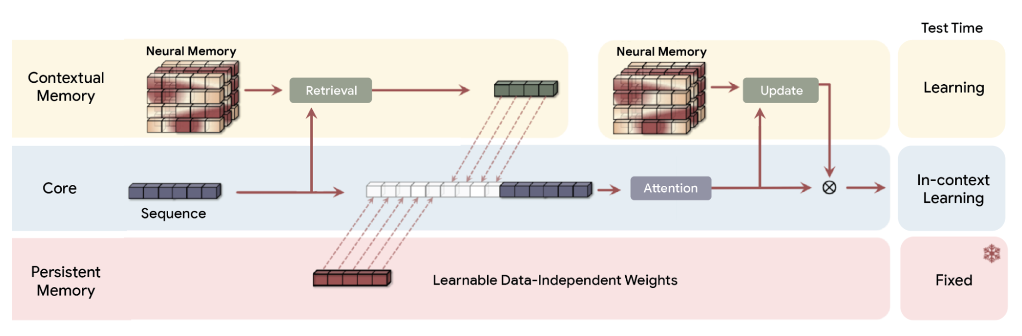
MIRAS treats memory as learnable parameters updated via local optimization with configurable loss functions (L1, L2, Huber). Training parallelizes via chunked sequences. The mathematical equivalence between RNN forget gates and weight decay reframes forgetting as a controllable design parameter. Loss function choice shapes memory stability: L2 overreacts to extreme tokens, while L1 or Huber creates more stable behavior.

Larimar (Das et al. 2024) adds distributed episodic memory to existing LLMs, enabling one-shot knowledge updates without retraining—achieving 8–10× speedups over traditional knowledge editing.

These architectures point toward systems that remember across sessions, update parameters during inference, and combine attention for immediate reasoning with neural memory for persistent knowledge. Where the field moved from RNN to LSTM to Transformer, Titans and MIRAS represent early signals of systems that bridge RNN efficiency with Transformer reasoning while adding persistent, adaptive memory.

Evaluation and Deployment

Effective context management requires measuring performance across three dimensions. Retrieval quality is assessed via Precision@k (fraction of top-\(k\) retrieved documents that are relevant), Recall (fraction of all relevant documents that were retrieved), and Mean Reciprocal Rank (average of \(1/\text{rank}\) for the first relevant result—higher when relevant documents appear earlier). Compression efficiency tracks compression ratio (original tokens divided by compressed tokens), task retention (performance on downstream tasks after compression), and latency improvements. Generation quality measures exact match accuracy (whether the answer matches a gold reference exactly), F1 scores (harmonic mean of precision and recall at the token level), and faithfulness—whether claims in the answer can be traced to the provided context rather than hallucinated. Libraries like RAGAS provide standardized evaluation pipelines for RAG systems, computing metrics such as faithfulness, answer relevancy, and context precision.

Different applications demand different context engineering strategies. Enterprise knowledge assistants typically employ hybrid retrieval (15 semantic + 5 BM25 candidates), cross-encoder reranking to the top-3, and LLMLingua-2 compression at 2–3×, targeting under 2,000 tokens of evidence with sub-500ms latency. Citations to retrieved chunks ensure auditability. Deep research systems favor hierarchical retrieval via RAPTOR for multi-level abstraction and GraphRAG for structural questions, synthesizing 5–10 documents while preserving source order. Codebase assistants combine sparse retrieval (symbols, filenames) with dense retrieval (conceptual similarity), limiting context to 3–5 surgical code blocks with aggressive caching of tool schemas, targeting under 4,000 tokens with sub-second latency.

A production deployment should address each stage systematically: chunking strategy matched to task requirements (small for lookup, large for narrative), hybrid search with metadata filtering, cross-encoder reranking to top-3 or top-5, high-relevance content positioned at context boundaries, compression applied to verbose content but skipped for structured data, static prompt components pinned via caching, tiered memory architecture for multi-turn workflows, and continuous monitoring of retrieval precision, token spend, and answer faithfulness.

24.12 Combining Techniques for Optimal Performance

The most effective AI systems combine these techniques strategically. An agent might follow structured prompts through instruction fine-tuning, think step-by-step using chain-of-thought reasoning, refine answers via reflexion, and align its tone through RLHF. This stacked approach has become standard: most large LLMs, including GPT-4, are first trained with supervised fine-tuning and then polished with RLHF.

Useful analogies: instruction fine-tuning is like teaching with flashcards; domain-specific fine-tuning resembles medical school specialization; chain-of-thought operates like showing your work in math class; tree-of-thought functions as decision tree exploration; reflexion mirrors learning from mistakes; RAG operates like an open-book exam; RLHF resembles teacher feedback; chain-of-action works like using tools while thinking.

In summary, the table below offers a concise overview of each post-training method. It includes simplified analogies to clarify the technical concepts, outlines the fundamental working principles, and highlights typical applications.

Post-training Method	Simplified Analogy	Basic Working Principle	Typical Applications
Instruction Fine-Tuning	Teaching with flashcards	Learning specific input-output patterns for following user commands	Following user commands
Domain-Specific Supervised Fine-Tuning	Medical school specialization	Absorbing field-specific vocabulary and rules for expert knowledge tasks	Expert knowledge tasks
Chain-of-Thought	Showing your work in math class	Generating intermediate reasoning steps for complex problem solving	Complex problem solving
Tree-of-Thought	Decision tree exploration	Branching and evaluating multiple paths for planning and strategy tasks	Planning and strategy tasks
Reflexion	Learning from mistakes	Writing a short reflection on what went wrong, then revising the approach	Iterative problem solving
Retrieval-Augmented Generation	An open-book exam, accessing external information for fact-based reasoning	Grabbing documents or information relevant to the query and injecting them into the context window so the model can reason over fresh evidence	Fact-based reasoning
Reinforcement Learning from Human Feedback	Teacher feedback, learning from human preferences for human-aligned responses	Taking a pre-trained model and generating several answers for real user prompts. Human reviewers rank those answers, a reward model learns these rankings, and the main model is updated to score higher on that reward	Human-aligned responses
Chain-of-Action	Using tools while thinking, interleaving reasoning with actions for multi-step tasks requiring external resources	Decomposing a complex query into a reasoning chain interleaved with tool calls such as web search, database lookup, or image retrieval that are executed on the fly and fed into the next thought	Multi-step tasks requiring external resources

Summary

Context management is a systems problem: chunking, retrieval, reranking, positioning, compression, and memory interact under a fixed budget. The engineering goal is simple—spend tokens on evidence and constraints that matter, not on redundancy.

Organizations deploying RAG without these optimizations leave substantial accuracy gains unrealized and pay more than necessary in API costs. The tools—LLMLingua-2, semantic chunking, cross-encoder reranking, prompt caching—are mature and open-source. What separates successful deployments is systematic application: measuring retrieval precision, compression ratios, and answer quality at each stage.

Emerging neural memory systems suggest a future beyond context window constraints—architectures that learn during inference and maintain persistent state across interactions. For now, context engineering remains essential: the difference between “it kind of works” and a reliable production system.

Ayala, Orlando, and Patrice Bechard. 2024. “Reducing Hallucination in Structured Outputs via Retrieval-Augmented Generation.” In Proceedings of the 2024 Conference of the North American Chapter of the Association for Computational Linguistics: Human Language Technologies (Volume 6: Industry Track), 228–38. Mexico City, Mexico: Association for Computational Linguistics.

Bai, Yuntao, Saurav Kadavath, Sandipan Kundu, Amanda Askell, Jackson Kernion, Andy Jones, Anna Chen, et al. 2022. “Constitutional AI: Harmlessness from AI Feedback.” arXiv. https://arxiv.org/abs/2212.08073.

Behrouz, Ali, and Mohammad Pezeshki. 2025. “MIRAS: Memory as an Optimization Object.” Google Research.

Behrouz, Ali, Mohammad Pezeshki, and Rasool Fakoor. 2025. “Titans: Learning to Memorize at Test Time.” arXiv Preprint arXiv:2501.00663. https://arxiv.org/abs/2501.00663.

Bird, Steven, Ewan Klein, and Edward Loper. 2009. Natural Language Processing with Python: Analyzing Text with the Natural Language Toolkit. Beijing ; Cambridge Mass.: O’Reilly Media.

Chen, Charlie, Sebastian Borgeaud, Jean-Baptiste Alayrac, Eliza Buchatskaya, Sebastian Bodnariu, Benoit Steiner, Junteng Jia, et al. 2023. “Accelerating Large Language Model Decoding with Speculative Sampling.” arXiv Preprint arXiv:2302.01318. https://arxiv.org/abs/2302.01318.

Chroma Research. 2024. “Evaluating Chunking Strategies for Retrieval.”

Chung, Hyung Won, Le Hou, Shayne Longpre, Barret Zoph, Yi Tay, William Fedus, Yunxuan Li, et al. 2022. “Scaling Instruction-Finetuned Language Models.” arXiv. https://arxiv.org/abs/2210.11416.

Dao, Tri. 2023. “FlashAttention-2: Faster Attention with Better Parallelism and Work Partitioning.” arXiv Preprint arXiv:2307.08691. https://arxiv.org/abs/2307.08691.

Das, Payel, Subhajit Chaudhury, Elliot Nelson, Igor Melnyk, Sarath Swaminathan, Sihui Dai, Aurélie Lozano, et al. 2024. “Larimar: Large Language Models with Episodic Memory Control.” In Proceedings of the 41st International Conference on Machine Learning (ICML).

Gao, Luyu, Xueguang Ma, Jimmy Lin, and Jamie Callan. 2022. “Precise Zero-Shot Dense Retrieval Without Relevance Labels.” arXiv Preprint arXiv:2212.10496. https://arxiv.org/abs/2212.10496.

Guan, Xinyu, Li Lyna Zhang, Yifei Liu, Ning Shang, Youran Sun, Yi Zhu, Fan Yang, and Mao Yang. 2025. “rStar-Math: Small LLMs Can Master Math Reasoning with Self-Evolved Deep Thinking.” arXiv. https://arxiv.org/abs/2501.04519.

Gupte, Mihir, Eshan Dixit, Muhammad Tayyab, and Arun Adiththan. 2025. “What Works for’lost-in-the-Middle’in Llms? A Study on GM-extract and Mitigations.” arXiv Preprint arXiv:2511.13900. https://arxiv.org/abs/2511.13900.

Hinton, Geoffrey, Oriol Vinyals, and Jeff Dean. 2015. “Distilling the Knowledge in a Neural Network.” arXiv Preprint arXiv:1503.02531. https://arxiv.org/abs/1503.02531.

Hou, Zhen, Hao Liu, Jiang Bian, Xing He, and Yan Zhuang. 2025. “Enhancing Medical Coding Efficiency Through Domain-Specific Fine-Tuned Large Language Models.” Npj Health Systems 2 (1): 14.

Hsieh, Cheng-Yu, Chun-Liang Li, Chih-Kuan Yeh, Hootan Nakhost, Yasuhisa Fujii, Alexander Ratner, Ranjay Krishna, Chen-Yu Lee, and Tomas Pfister. 2023. “Distilling Step-by-Step! Outperforming Larger Language Models with Less Training Data and Smaller Model Sizes.” arXiv Preprint arXiv:2305.02301. https://arxiv.org/abs/2305.02301.

Jiang, Huiqiang, Qianhui Wu, Chin-Yew Lin, Yuqing Yang, and Lili Qiu. 2023. “LLMLingua: Compressing Prompts for Accelerated Inference of Large Language Models.” arXiv Preprint arXiv:2310.05736. https://arxiv.org/abs/2310.05736.

Khattab, Omar, and Matei Zaharia. 2020. “ColBERT: Efficient and Effective Passage Search via Contextualized Late Interaction over BERT.” In Proceedings of the 43rd International ACM SIGIR Conference on Research and Development in Information Retrieval, 39–48. ACM.

Leviathan, Yaniv, Matan Kalman, and Yossi Matias. 2023. “Fast Inference from Transformers via Predictive Sampling.” arXiv Preprint arXiv:2211.17191. https://arxiv.org/abs/2211.17191.

Liu, Hao, Matei Zaharia, and Pieter Abbeel. 2023. “Ring Attention with Blockwise Transformers for Near-Infinite Context.” arXiv Preprint arXiv:2310.01889. https://arxiv.org/abs/2310.01889.

Liu, Nelson F., Kevin Lin, John Hewitt, Ashwin Paranjape, Michele Bevilacqua, Fabio Petroni, and Percy Liang. 2024. “Lost in the Middle: How Language Models Use Long Contexts.” Transactions of the Association for Computational Linguistics 12: 157–73.

Microsoft Research. 2024. “GraphRAG: Unlocking LLM Discovery on Narrative Private Data.”

Ouyang, Long, Jeffrey Wu, Xu Jiang, Diogo Almeida, Carroll Wainwright, Pamela Mishkin, Chong Zhang, et al. 2022. “Training Language Models to Follow Instructions with Human Feedback.” Advances in Neural Information Processing Systems 35: 27730–44.

Packer, Charles, Vivian Fang, Shishir G. Patil, Kevin Lin, Sarah Wooders, and Joseph E. Gonzalez. 2023. “MemGPT: Towards LLMs as Operating Systems.” arXiv Preprint arXiv:2310.08560. https://arxiv.org/abs/2310.08560.

Pan, Zhenyu, Haozheng Luo, Manling Li, and Han Liu. 2025. “Chain-of-Action: Faithful and Multimodal Question Answering Through Large Language Models.” arXiv. https://arxiv.org/abs/2403.17359.

Rafailov, Rafael, Archit Sharma, Eric Mitchell, Stefano Ermon, Christopher D. Manning, and Chelsea Finn. 2023. “Direct Preference Optimization: Your Language Model Is Secretly a Reward Model.” arXiv. https://arxiv.org/abs/2305.18290.

Sanh, Victor, Lysandre Debut, Julien Chaumond, and Thomas Wolf. 2019. “DistilBERT, a Distilled Version of BERT: Smaller, Faster, Cheaper and Lighter.” arXiv Preprint arXiv:1910.01108. https://arxiv.org/abs/1910.01108.

Sarthi, Parth, Salman Abdullah, Aditi Tuli, Shubh Khanna, Anna Goldie, and Christopher D. Manning. 2024. “RAPTOR: Recursive Abstractive Processing for Tree-Organized Retrieval.” arXiv Preprint arXiv:2401.18059. https://arxiv.org/abs/2401.18059.

Shinn, Noah, Federico Cassano, Edward Berman, Ashwin Gopinath, Karthik Narasimhan, and Shunyu Yao. 2023. “Reflexion: Language Agents with Verbal Reinforcement Learning.” https://arxiv.org/abs/2303.11366.

Wei, Jason, Xuezhi Wang, Dale Schuurmans, Maarten Bosma, Brian Ichter, Fei Xia, Ed Chi, Quoc Le, and Denny Zhou. 2023. “Chain-of-Thought Prompting Elicits Reasoning in Large Language Models.” arXiv. https://arxiv.org/abs/2201.11903.

Yang, An, Bowen Yu, Chengyuan Li, Dayiheng Liu, Fei Huang, Haoyan Huang, Jiandong Jiang, et al. 2025. “Qwen2. 5-1m Technical Report.” arXiv Preprint arXiv:2501.15383. https://arxiv.org/abs/2501.15383.

Yao, Shunyu, Dian Yu, Jeffrey Zhao, Izhak Shafran, Thomas L. Griffiths, Yuan Cao, and Karthik Narasimhan. 2023. “Tree of Thoughts: Deliberate Problem Solving with Large Language Models.” arXiv. https://arxiv.org/abs/2305.10601.

Ye, Yixin, Zhen Huang, Yang Xiao, Ethan Chern, Shijie Xia, and Pengfei Liu. 2025. “LIMO: Less Is More for Reasoning.” arXiv. https://arxiv.org/abs/2502.03387.

Yu, Gyeong-In, Joo Seong Jeong, Geon-Woo Kim, Soo-Jin Jeong, Woosung Lee, and Byung-Gon Chun. 2022. “Orca: A Distributed Serving System for Transformer-based Generative Models.” In 16th USENIX Symposium on Operating Systems Design and Implementation (OSDI 22), 527–46.