23  Natural Language Processing

CNNs (Chapter 22) exploited the spatial structure of images; language presents a different kind of structure. Words are discrete symbols; their meaning depends on context, and sentences have variable length. These properties demand a new set of architectural ideas—embeddings, attention, and the Transformer—developed in this chapter.

The ability to understand and generate human language has long been considered a hallmark of intelligence. When Alan Turing proposed his famous test in 1950, he chose natural conversation as the ultimate benchmark for machine intelligence. Yet for decades, this goal remained frustratingly elusive. Early attempts at machine translation in the 1950s, which simply replaced words using bilingual dictionaries, produced nonsensical results that highlighted the complexity of human language. The phrase “The spirit is willing, but the flesh is weak” allegedly translated to Russian and back as “The vodka is good, but the meat is rotten”: a cautionary tale about the subtleties of meaning that transcend mere word substitution.

This chapter traces the path from those early failures to today’s language models that can engage in nuanced dialogue, translate between languages with near-human accuracy, and even generate creative text. At the heart of this transformation lies a fundamental shift in how we represent language computationally: from discrete symbols manipulated by hand-crafted rules to continuous vector spaces learned from vast corpora of text.

The chapter develops the mathematical foundations of natural language understanding: word embeddings, attention mechanisms, and the Transformer architecture that powers modern language models like BERT and GPT.

23.1 Converting Words to Numbers (Embeddings)

Language poses distinctive challenges for mathematical modeling: unlike images, which naturally exist as arrays of continuous pixel values, or audio signals, which are continuous waveforms, text consists of discrete symbols with no inherent geometric structure. The word “cat” is not inherently closer to “dog” than to “quantum”, at least not in any obvious mathematical sense. Yet humans effortlessly recognize that cats and dogs share semantic properties that neither shares with abstract physics concepts.

A naive way to represent words is through one-hot encoding, where each word in a vocabulary is assigned a unique vector with a single non-zero entry. For example, in a vocabulary of size \(|V|\), the word “cat” might be represented as \[ v_{\text{cat}} = \overbrace{[0, 0, \ldots, 1, \ldots, 0]}^{|V|} \] with the 1 in the \(i\)-th position corresponding to “cat”. However, this approach fails to capture any notion of semantic similarity: the cosine similarity between any two distinct one-hot vectors is zero, erasing all information about how words relate to each other.

This type of representation makes even the seemingly simple task of determining whether two sentences have similar meanings challenging. The sentences “The cat sat on the mat” and “A feline rested on the rug” express nearly identical ideas despite sharing no words except “the” and “on.” Conversely, “The bank is closed” could refer to a financial institution or a river’s edge, with the same words encoding entirely different meanings. These examples illustrate why early symbolic approaches to natural language processing, based on logical rules and hand-crafted features, struggled to capture the fluid, contextual nature of meaning.

The breakthrough came from reconceptualizing the representation problem. Instead of treating words as atomic symbols, we embed them in a continuous vector space where geometric relationships encode semantic relationships. In such a space, we might find that \(v_{\text{cat}} - v_{\text{dog}}\) has a similar direction to \(v_{\text{car}} - v_{\text{bicycle}}\), capturing analogical relationships through vector arithmetic.

To formalize this intuition, we seek a mapping \(\phi: \mathcal{V} \rightarrow \mathbb{R}^d\) from a vocabulary \(\mathcal{V}\) of discrete tokens to \(d\)-dimensional vectors. The challenge lies in learning this mapping such that the resulting geometry reflects semantic relationships.

The Math of Twenty Questions

My (Vadim’s) daughter and I play a game of Twenty Questions during road trips. The rules are simple: one person thinks of something, and the other person has to guess what it is by asking yes-or-no questions. The person who is guessing can ask up to twenty questions, and then they have to make a guess. If they guess correctly, they win; if not, the other person wins. The game is fun, but it’s also a great way to illustrate how AI systems can learn to represent words and phrases as numbers. The trick is to come up with an optimal set of yes-or-no questions that will allow you to distinguish between all the words or phrases you might want to represent. Surprisingly, most of the words can be identified with a small set of universal questions asked in the same order every time. Usually the person who has a better set of questions wins. For example, you might ask:

• Is it an animal? (Yes)
• Is this a domestic animal? (No)
• Is it larger than a human? (Yes)
• Does it have a long tail? (No)
• Is it a predator? (Yes)
• Can it move on two feet? (Yes)
• Is it a bear? (Yes)

Thus, if we use a 20-dimensional 0-1 vector to represent the word “bear,” the portion of this vector corresponding to these questions would look like this:

	Animal	Domestic	Larger than human	Long tail	Predator	Can move on two feet
Bear	1	0	1	0	1	1

This is called a word vector. Specifically, it’s a “binary” or 0/1 vector: 1 means yes, 0 means no. Different words would produce different answers to the same questions, so they would have different word vectors. If we stack all these vectors in a matrix, where each row is a word, and each column is a question, we get something like this:

	Animal	Domestic	Larger than human	Long tail	Predator	Can move on two feet
Bear	1	0	1	0	1	1
Dog	1	1	0	1	0	0
Cat	1	1	0	1	1	0

The binary nature of these vectors forces us to choose 1 or 0 for the “Larger than human” question for “Dog.” However, there are some dog breeds that are larger than humans, so this binary representation is not very useful in this case. We can do better by allowing the answers to be numbers between 0 and 1, rather than just 0 or 1. This way, we can represent the fact that some dogs are larger than humans, but most are not. For example, we might answer the question “Is it larger than a human?” with a 0.1 for a dog and a 0.8 for a bear. Some types of bears can be smaller than humans, for example, black bears that live in North America, but most bears are larger than humans.

Using this approach, the vectors now become

	Animal	Domestic	Larger than human	Long tail	Predator	Can move on two feet
Bear	1	0	0.8	0	1	0.8
Dog	1	1	0.1	0.6	0	0
Cat	1	0.7	0.01	1	0.6	0

AI systems also use non-binary scoring rules to judge a win or loss. For example, if the answer is “bear,” then the score might be 100 points for a correct guess, 90 points for a close guess like “wolf” or “lion,” and 50 points for a distant guess like “eagle.” This way of keeping score matches the real-world design requirements of most NLP systems. For example, if you translate JFK saying “Ich bin ein Berliner” as “I am a German,” you’re wrong, but a lot closer than if you translate it as “I am a butterfly.”

The process of converting words into numbers is called “embedding.” The resulting vectors are called “word embeddings.” The only part that is left is how to design an algorithm that can find a good set of questions to ask. Usually real-life word embeddings have hundreds of questions, not just twenty. The process of finding these questions is called “training” the model. The goal is to find a set of questions that will allow the model to distinguish between all the words in the vocabulary, and to do so in a way that captures their meanings. However, the algorithms do not have a notion of meaning in the same way that humans do. Instead, they learn by counting word co-location statistics—that is, which words tend to appear with which other words in real sentences written by humans.

These co-occurrence statistics serve as surprisingly effective proxies for meaning. For example, consider the question: “Among all sentences containing ‘fries’ and ‘ketchup,’ how frequently does the word ‘bun’ also appear?” This is the kind of query a machine can easily formulate and answer, since it relies on counting rather than true understanding.

While such a specific question may be too limited if you can only ask a few hundred, the underlying idea—using word co-occurrence patterns—is powerful. Word embedding algorithms are built on this principle: they systematically explore which words tend to appear together, and through optimization, learn the most informative “questions” to ask. By repeatedly applying these learned probes, the algorithms construct a vector for each word or phrase, capturing its relationships based on co-occurrence statistics. These word vectors are then organized into a matrix for further use.

There are many ways to train word embeddings, but the most common one is to use a neural network. The neural network learns to ask questions that are most useful for distinguishing between different words. It does this by sweeping through millions of sentences and nudging each word’s vector so that the word predicts the words next to it. Nothing labels the meanings: the surrounding text is the only supervision. One of the most influential algorithms for this is Word2Vec, introduced by Mikolov et al. (2013) at Google in 2013. Earlier neural language models had used distributed word representations, but Word2Vec’s efficiency and scale made it the standard approach for pre-trained embeddings.

23.2 Word2Vec and Distributional Semantics

The theoretical foundation for learning meaningful word representations comes from the distributional hypothesis, articulated by linguist J.R. Firth in 1957: “You shall know a word by the company it keeps” (Firth 1957). This principle suggests that words appearing in similar contexts tend to have similar meanings. If “coffee” and “tea” both frequently appear near words like “drink,” “hot,” “cup,” and “morning,” we can infer their semantic similarity.

The word2vec framework, introduced by Mikolov et al. (2013), operationalized this insight through a probabilistic model. The skip-gram variant posits that a word can be used to predict its surrounding context words. Given a corpus of text represented as a sequence of words \(w_1, w_2, \ldots, w_T\), the model maximizes the likelihood:

\[\mathcal{L} = \sum_{t=1}^T \sum_{-m \leq j \leq m, j \neq 0} \log P(w_{t+j} \mid w_t)\]

where \(m\) is the context window size. The conditional probability is parameterized using two sets of embeddings: \(\mathbf{v}_w\) for words as centers and \(\mathbf{u}_w\) for words as context:

\[P(w_o \mid w_c) = \frac{\exp(\mathbf{u}_o^\top \mathbf{v}_c)}{\sum_{w \in \mathcal{V}} \exp(\mathbf{u}_w^\top \mathbf{v}_c)}\]

This formulation reveals deep connections to the theoretical frameworks discussed in previous chapters. The dot product \(\mathbf{u}_o^\top \mathbf{v}_c\) acts as a compatibility score between center and context words, while the softmax normalization ensures a valid probability distribution. From the perspective of ridge functions, we can view this as learning representations where the function \(f(w_c, w_o) = \mathbf{u}_o^\top \mathbf{v}_c\) captures the log-odds of co-occurrence.

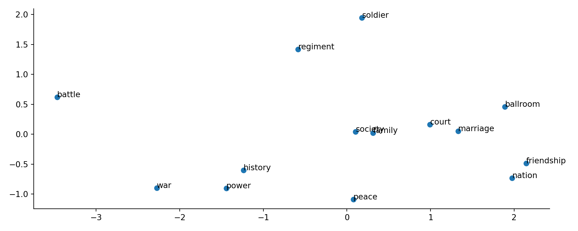
Word2Vec for War and Peace. This analysis applies Word2Vec to Leo Tolstoy’s “War and Peace,” demonstrating how neural network-based techniques can learn vector representations of words by analyzing their contextual relationships within the text. The model employs the continuous bag-of-words (CBOW) algorithm with negative sampling (explained later), the default configuration in gensim and a widely used setup for Word2Vec. We use a vector dimension of 100, providing a balance between capturing semantic detail and computational efficiency. The context window size is set to 5, and the model is trained over several iterations to ensure convergence. Finally, we use PCA to reduce the dimensionality of the vectors to 2D for visualization.

Word2Vec for War and Peace.

The results reveal meaningful semantic relationships within the text and highlight several key insights into the thematic structure of Tolstoy’s War and Peace. First, the clustering of military-related terms (soldier, regiment, battle) underscores Word2Vec’s ability to group semantically related words based on their co-occurrence patterns. Additionally, the grouping of words such as “ballroom,” “court,” and “marriage” reflects the novel’s emphasis on aristocratic society and its social hierarchy. The use of PCA for dimensionality reduction effectively preserves meaningful relationships while reducing the original high-dimensional Word2Vec space (100 dimensions) to a two-dimensional representation. Overall, this visualization demonstrates how Word2Vec captures distinct thematic domains, including military, social, and government. Notice that a more abstract concept like peace is surrounded by words from both government (history, power, war) and social domains (family, friendship, marriage,court, ballroom, society), indicating its central role in the narrative but is distant from the military domain, which is more focused on the war aspect of the story.

These insights have practical applications in literary analysis, theme extraction, character relationship mapping, historical text understanding, and similarity-based text search and recommendation systems.

The Skip-Gram Model

The skip-gram model predicts surrounding context words within a fixed window given a center word. This approach assumes that words appearing in similar contexts tend to have similar meanings, directly implementing the distributional hypothesis.

Consider the sentence “The man loves his son” with “loves” as the center word and a context window of size 2. The skip-gram model aims to maximize the probability of generating the context words “the,” “man,” “his,” and “son” given the center word “loves.” This relationship can be visualized as follows:

graph TD
    A[loves] --> B[the]
    A --> C[man]
    A --> D[his]
    A --> E[son]
    
    style A fill:#e1f5fe
    style B fill:#f3e5f5
    style C fill:#f3e5f5
    style D fill:#f3e5f5
    style E fill:#f3e5f5
    
    classDef centerWord fill:#e1f5fe,stroke:#0277bd,stroke-width:2px
    classDef contextWord fill:#f3e5f5,stroke:#7b1fa2,stroke-width:2px
    
    class A centerWord
    class B,C,D,E contextWord

The mathematical foundation assumes conditional independence among context words given the center word, allowing the joint probability to factorize:

\[ \begin{aligned} &P(\text{"the"}, \text{"man"}, \text{"his"}, \text{"son"} \mid \text{"loves"}) = \\ &\quad P(\text{"the"} \mid \text{"loves"}) \cdot P(\text{"man"} \mid \text{"loves"}) \cdot P(\text{"his"} \mid \text{"loves"}) \cdot P(\text{"son"} \mid \text{"loves"}) \end{aligned} \]

This independence assumption, while not strictly true in natural language, is needed for computational tractability. Each conditional probability is modeled using the softmax function over the entire vocabulary:

\[P(w_o \mid w_c) = \frac{\exp(\mathbf{u}_o^\top \mathbf{v}_c)}{\sum_{i \in \mathcal{V}} \exp(\mathbf{u}_i^\top \mathbf{v}_c)}\]

The skip-gram objective seeks to maximize the likelihood of observing all context words across the entire corpus. For a text sequence of length \(T\) with words \(w^{(1)}, w^{(2)}, \ldots, w^{(T)}\), the objective becomes:

\[\mathcal{L}_{\text{skip-gram}} = \frac{1}{T} \sum_{t=1}^T \sum_{-m \leq j \leq m, j \neq 0} \log P(w^{(t+j)} \mid w^{(t)})\]

where \(m\) is the context window size. The normalization by \(T\) ensures that the objective remains bounded as corpus size grows.

The gradient with respect to the center word embedding reveals the learning dynamics:

\[\frac{\partial \log P(w_o \mid w_c)}{\partial \mathbf{v}_c} = \mathbf{u}_o - \sum_{i \in \mathcal{V}} P(w_i \mid w_c) \mathbf{u}_i\]

The gradient pushes the center word embedding toward the observed context word (\(\mathbf{u}_o\)) while pulling it away from all other words, weighted by their predicted probabilities. This creates a natural contrast between positive and negative examples.

The skip-gram architecture assigns two vector representations to each word: \(\mathbf{v}_w\) when the word serves as a center word and \(\mathbf{u}_w\) when it appears in context. This asymmetry allows the model to capture different aspects of word usage. After training, the center word vectors \(\mathbf{v}_w\) are typically used as the final word embeddings, though some implementations average or concatenate both representations.

The Continuous Bag of Words (CBOW) Model

While skip-gram predicts context words from a center word, the Continuous Bag of Words (CBOW) model reverses this relationship: it predicts a center word based on its surrounding context. For the same text sequence “the”, “man”, “loves”, “his”, “son” with “loves” as the center word, CBOW models the conditional probability:

\[P(\text{"loves"} \mid \text{"the"}, \text{"man"}, \text{"his"}, \text{"son"})\]

The CBOW architecture can be visualized as multiple context words converging to predict a single center word:

graph TD
    B[the] --> A[loves]
    C[man] --> A
    D[his] --> A
    E[son] --> A
    
    style A fill:#e1f5fe
    style B fill:#f3e5f5
    style C fill:#f3e5f5
    style D fill:#f3e5f5
    style E fill:#f3e5f5
    
    classDef centerWord fill:#e1f5fe,stroke:#0277bd,stroke-width:2px
    classDef contextWord fill:#f3e5f5,stroke:#7b1fa2,stroke-width:2px
    
    class A centerWord
    class B,C,D,E contextWord

The key difference from skip-gram lies in how CBOW handles multiple context words. Rather than treating each context word independently, CBOW averages their embeddings. For a center word \(w_c\) with context words \(w_{o_1}, \ldots, w_{o_{2m}}\), the conditional probability is:

\[P(w_c \mid w_{o_1}, \ldots, w_{o_{2m}}) = \frac{\exp\left(\mathbf{u}_c^\top \bar{\mathbf{v}}_o\right)}{\sum_{i \in \mathcal{V}} \exp\left(\mathbf{u}_i^\top \bar{\mathbf{v}}_o\right)}\]

where \(\bar{\mathbf{v}}_o = \frac{1}{2m}\sum_{j=1}^{2m} \mathbf{v}_{o_j}\) is the average of context word vectors. Note that in CBOW, \(\mathbf{u}_i\) represents word \(i\) as a center word, and \(\mathbf{v}_i\) represents it as a context word, the opposite of skip-gram’s convention.

The CBOW objective maximizes the likelihood of generating all center words given their contexts:

\[\mathcal{L}_{\text{CBOW}} = \sum_{t=1}^T \log P(w^{(t)} \mid w^{(t-m)}, \ldots, w^{(t-1)}, w^{(t+1)}, \ldots, w^{(t+m)})\]

The gradient with respect to context word vectors reveals how CBOW learns:

\[\frac{\partial \log P(w_c \mid \mathcal{W}_o)}{\partial \mathbf{v}_{o_i}} = \frac{1}{2m}\left(\mathbf{u}_c - \sum_{j \in \mathcal{V}} P(w_j \mid \mathcal{W}_o) \mathbf{u}_j\right)\]

This gradient is scaled by \(\frac{1}{2m}\), effectively distributing the learning signal across all context words. CBOW tends to train faster than skip-gram because it predicts one word per context window rather than multiple words, but skip-gram often produces better representations for rare words since it generates more training examples per sentence.

Pretraining Word2Vec

Training word2vec models requires careful attention to implementation details that significantly impact the quality of learned representations. The training process begins with data preprocessing on large text corpora. Using the Penn Treebank dataset as an example (a carefully annotated corpus of Wall Street Journal articles containing about 1 million words), we implement several key preprocessing steps.

First, we build a vocabulary by counting word frequencies and retaining only words that appear at least a minimum number of times (typically 5-10). This thresholding serves two purposes: it reduces the vocabulary size from potentially millions to tens of thousands of words, and it prevents the model from wasting capacity on rare words that appear too infrequently to learn meaningful representations. Words below the threshold are replaced with a special <unk> token.

The training procedure uses stochastic gradient descent with a carefully designed learning rate schedule. The initial learning rate (typically 0.025 for skip-gram and 0.05 for CBOW) is linearly decreased to a minimum value (usually 0.0001) as training progresses:

\[\alpha_t = \alpha_0 \left(1 - \frac{\text{words\_processed}}{\text{total\_words} \times \text{epochs}}\right)\]

This schedule ensures larger updates early in training when representations are poor, transitioning to fine-tuning as the model converges.

The implementation uses several optimizations for efficiency. Word vectors are typically initialized randomly from a uniform distribution over \([-0.5/d, 0.5/d]\) where \(d\) is the embedding dimension (commonly 100-300). During training, we maintain two embedding matrices: one for center words and one for context words. After training, these can be combined (usually by averaging) or just the center word embeddings can be used.

For minibatch processing, training examples are grouped to enable efficient matrix operations. Given a batch of center-context pairs, the forward pass computes scores using matrix multiplication, applies the loss function (either full softmax, hierarchical softmax, or negative sampling), and backpropagates gradients. A typical training configuration might process batches of 512 word pairs, iterating 5-15 times over a corpus.

The quality of learned embeddings can be evaluated through word similarity and analogy tasks. For similarity, we compute cosine distances between word vectors and verify that semantically similar words have high cosine similarity. For analogies, we test whether vector arithmetic captures semantic relationships: the famous “king - man + woman \(\approx\) queen” example demonstrates that vector differences encode meaningful semantic transformations.

An important but often overlooked aspect is subsampling of frequent words. Words like “the,” “a,” and “is” appear so frequently that they provide little information about the semantic content of their neighbors. The probability of discarding a word \(w\) during training is:

\[P(\text{discard } w) = 1 - \sqrt{\frac{t}{f(w)}}\]

where \(f(w)\) is the frequency of word \(w\) and \(t\) is a threshold (typically \(10^{-5}\)). This formula ensures that very frequent words are aggressively subsampled while preserving most occurrences of informative words.

For training, we extract examples by sliding a window over the text. For each center word, we collect its context words within a window of size \(m\). Importantly, the actual window size is sampled uniformly from \([1, m]\) for each center word, which helps the model learn representations that are robust to varying context sizes. Consider the sentence “the cat sat on the mat” with maximum window size 2. For the center word “sat,” we might sample a window size of 1, giving context words [“cat”, “on”], or a window size of 2, giving context words [“the”, “cat”, “on”, “the”].

23.3 Computational Efficiency through Negative Sampling

The elegance of word2vec’s formulation belies a serious computational challenge. Computing the normalization term in the softmax requires summing over the entire vocabulary (potentially millions of terms) for every gradient update. With large corpora containing billions of words, this quickly becomes intractable.

Negative sampling transforms the problem from multi-class classification to binary classification. Instead of predicting which word from the entire vocabulary appears in the context, we ask a simpler question: given a word pair, is it a real center-context pair from the corpus or a randomly generated negative example? The objective becomes:

\[\mathcal{L}_{\text{NS}} = \log \sigma(\mathbf{u}_o^\top \mathbf{v}_c) + \sum_{k=1}^K \E[w_k \sim P_n]{\log \sigma(-\mathbf{u}_{w_k}^\top \mathbf{v}_c)}\]

where \(\sigma(x) = 1/(1 + e^{-x})\) is the sigmoid function, and \(P_n\) is a noise distribution over words. Each update now touches \(K+1\) vectors instead of \(|\mathcal{V}|\), with \(K\) typically between 5 and 20. Negative sampling does not approximate the softmax likelihood; it replaces it. Its optimum satisfies \(\mathbf{u}_o^\top \mathbf{v}_c = \mathrm{PMI}(o, c) - \log K\) (Levy and Goldberg 2014), so the learned vectors factor a shifted pointwise-mutual-information matrix rather than the skip-gram conditional distribution. The noise distribution is set empirically to \(P_n(w) \propto f(w)^{3/4}\), where \(f(w)\) is word frequency; the exponent draws frequent words less often than their raw frequency would, and was chosen by experiment rather than derived.

An alternative solution is hierarchical softmax, which replaces the flat softmax over the vocabulary with a binary tree where each leaf represents a word. The probability of a word is then the product of binary decisions along the path from root to leaf:

\[P(w_o \mid w_c) = \prod_{j=1}^{L(w_o)-1} \sigma\left([\![n(w_o, j+1) = \text{leftChild}(n(w_o, j))]\!] \cdot \mathbf{u}_{n(w_o,j)}^\top \mathbf{v}_c\right)\]

where \(L(w_o)\) is the length of the path to word \(w_o\), \(n(w_o, j)\) is the \(j\)-th node on this path, and \([\![\cdot]\!]\) is the Iverson bracket—a notation that returns \(+1\) if the condition inside is true (the next node is the left child) and \(-1\) otherwise (the next node is the right child). This sign flip determines whether we use the sigmoid or its complement at each binary decision. Hierarchical softmax reduces computational complexity from \(O(|\mathcal{V}|)\) to \(O(\log |\mathcal{V}|)\), though negative sampling typically performs better in practice.

23.4 Global Vectors and Matrix Factorization

While word2vec learns from local context windows, GloVe (Global Vectors) (Pennington, Socher, and Manning 2014) leverages global co-occurrence statistics. The key observation is that the ratio of co-occurrence probabilities can encode semantic relationships. Consider the words “ice” and “steam” in relation to “solid” and “gas”: \(P(\text{solid} \mid \text{ice}) / P(\text{solid} \mid \text{steam})\) is large (around 8.9), while \(P(\text{gas} \mid \text{ice}) / P(\text{gas} \mid \text{steam})\) is small (around 0.085), and \(P(\text{water} \mid \text{ice}) / P(\text{water} \mid \text{steam})\) is close to 1 (around 1.36).

These ratios capture the semantic relationships: ice is solid, steam is gas, and both relate to water. GloVe learns embeddings that preserve these ratios through the objective:

\[\mathcal{L}_{\text{GloVe}} = \sum_{i,j} h(X_{ij}) \left(\mathbf{v}_i^\top \mathbf{u}_j + b_i + c_j - \log X_{ij}\right)^2\]

where \(X_{ij}\) counts co-occurrences, \(h(\cdot)\) is a weighting function that prevents very common or very rare pairs from dominating, and \(b_i, c_j\) are bias terms. A typical choice is \(h(x) = (x/x_{\max})^{\alpha}\) if \(x < x_{\max}\), else 1, with \(\alpha = 0.75\) and \(x_{\max} = 100\).

This formulation reveals GloVe as a weighted matrix factorization problem. We seek low-rank factors \(\mathbf{V}\) and \(\mathbf{U}\) such that \(\mathbf{V}^\top\mathbf{U} \approx \log \mathbf{X}\), where the approximation is weighted by the function \(h(\cdot)\). With \(h \equiv 1\) and no bias terms, the minimizer is the truncated SVD of \(\log \mathbf{X}\), by the Eckart-Young theorem. The weights \(h(X_{ij})\) destroy that closed form: weighted low-rank approximation has no eigendecomposition solution in general, which is why GloVe is fitted by gradient descent (AdaGrad) rather than by an SVD. The unweighted case is still the right intuition for what the factors represent.

23.5 Beyond Words: Subword and Character Models (Tokenization)

A fundamental limitation of word-level embeddings is their inability to handle out-of-vocabulary words or capture morphological relationships. The word “unhappiness” shares obvious morphological connections with “happy,” “unhappy,” and “happiness,” but word2vec treats these as completely independent tokens.

FastText (Bojanowski et al. 2017) addresses this limitation by representing words as bags of character n-grams. For the word “where” with n-grams of length 3 to 6, we extract: “<wh”, “whe”, “her”, “ere”, “re>”, and longer n-grams up to the full word. The word embedding is then the sum of its n-gram embeddings:

\[\mathbf{v}_{\text{where}} = \sum_{g \in \mathcal{G}_{\text{where}}} \mathbf{z}_g\]

This approach handles out-of-vocabulary words by breaking them into known n-grams and provides better representations for rare words by sharing parameters across morphologically related words.

An even more flexible approach is Byte Pair Encoding (BPE), which learns a vocabulary of subword units directly from the data. Starting with individual characters, BPE iteratively merges the most frequent pair of adjacent units until reaching a desired vocabulary size. For example, given a corpus with word frequencies {“fast”: 4, “faster”: 3, “tall”: 5, “taller”: 4}, BPE might learn merges like “t” + “a” \(\rightarrow\) “ta”, then “ta” + “l” \(\rightarrow\) “tal”, and so on. This data-driven approach balances vocabulary size with representation power, enabling models to handle arbitrary text while maintaining reasonable computational requirements.

The choice of tokenization strategy has direct implications for model performance and behavior. Modern LLMs typically use vocabularies of 50,000 to 100,000 tokens, carefully balanced to represent different languages while maintaining computational efficiency. A vocabulary that’s too small forces the model to represent complex concepts with many tokens, making it harder to capture meaning efficiently.

Consider how “The Verbasizer helped Bowie create unexpected word combinations” might be tokenized: [“The”, ” Ver”, “bas”, “izer”, ” helped”, ” Bow”, “ie”, ” create”, ” unexpected”, ” word”, ” combinations”]. This fragmentation handles rare words and proper names by breaking them into common subcomponents.

This tokenization process explains some behavioral patterns in modern language models. Names from fictional universes, specialized terminology, and code snippets can be tokenized in ways that fragment their semantic meaning, potentially affecting model performance.

23.6 Attention Mechanisms and Contextual Representations

In Chapter 19, we interpreted attention as a form of kernel smoothing. Here we develop the full architecture from first principles.

Static word embeddings suffer from a fundamental limitation: they assign a single vector to each word, ignoring context. The word “bank” receives the same representation whether it appears in “river bank” or “investment bank.” This conflation of multiple senses into a single vector creates an information bottleneck that limits performance on downstream tasks.

The evolution of word embeddings culminated in contextual representations, which dynamically adjust based on surrounding context. The context problem was solved by attention mechanisms, particularly the transformer architecture, which allows models to capture complex dependencies between words. Attention mimics the human ability to selectively focus: when reading, your visual system processes every word simultaneously, yet conscious attention flows sequentially. You can redirect this attention at will—noticing a particular phrase or jumping back to reread a complex clause.

Machine learning systems faced analogous challenges in processing sequential information. Early neural networks, particularly recurrent architectures, processed sequences step by step, maintaining a hidden state that theoretically encoded all previous information. However, this sequential bottleneck created fundamental limitations: information from early time steps could vanish as sequences grew longer, and the inherently sequential nature prevented parallel computation that could exploit modern hardware effectively.

The attention (Bahdanau, Cho, and Bengio 2014; Vaswani et al. 2017) mechanism reshaped this landscape by allowing models to directly access and combine information from any part of the input sequence. Rather than compressing an entire sequence into a fixed-size vector, attention mechanisms create dynamic representations that adaptively weight different parts of the input based on their relevance to the current computation. This breakthrough enabled the development of the Transformer architecture, which forms the foundation of modern language models from BERT to GPT.

At its core, attention implements an information retrieval system inspired by database operations. Consider how you might search through a library: you formulate a query (what you’re looking for), examine the keys (catalog entries or book titles), and retrieve the associated values (the actual books or their contents). Attention mechanisms formalize this intuition through three learned representations:

• Queries (\(\mathbf{Q}\)): What information are we seeking?
• Keys (\(\mathbf{K}\)): What information is available at each position?
• Values (\(\mathbf{V}\)): What information should we retrieve?

Given a set of keys and values, attention computes a weighted sum of the values based on their relevance to the query. Mathematically, this can be expressed as: \[ \textrm{Attention}(\mathbf{q}) \defeq \sum_{i=1}^m \alpha_i(\mathbf{q}, \mathbf{k}_i) \mathbf{v}_i, \]

where \(\alpha_i\) are scalar attention weights computed from the queries and keys. The operation itself is typically referred to as attention pooling. The name “attention” derives from the fact that the operation pays particular attention to the terms for which the weight \(\alpha_i\) is significant (i.e., large).

It is typical in AI applications to assume that the attention weights \(\alpha_i\) are nonnegative and form a convex combination, i.e., \(\sum_{i=1}^m \alpha_i = 1\). A common strategy for ensuring that the weights sum up to 1 is to normalize the unnormalized scores \(s_i\) via the softmax function: \[ \alpha_i = \frac{\exp(s_i)}{\sum_{j=1}^m \exp(s_j)} \]

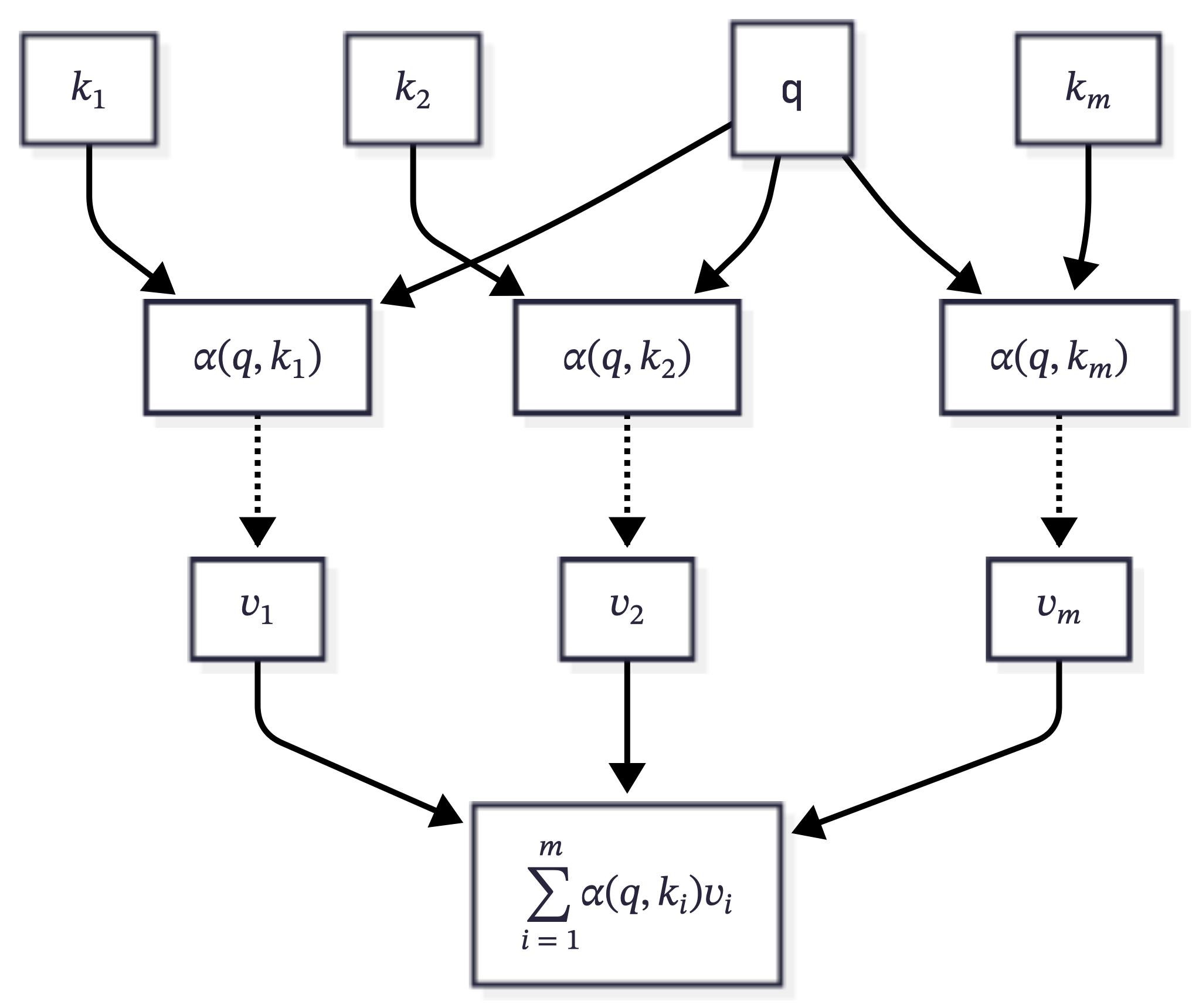
This diagram shows the basic attention computation. A query vector \(q\) is compared to each key \(k_i\) to produce a score, which is then turned into an attention weight \(\alpha(q,k_i)\) (often normalized so the weights sum to one). The output is a weighted sum of the value vectors, \(\sum_{i=1}^m \alpha(q,k_i) v_i\), so values associated with keys most relevant to the query contribute more to the final representation.

Kernel smoothing as attention. The concept of attention pooling can be traced back to classical kernel methods like Nadaraya-Watson regression, where similarity kernels determine how much weight to give to different data points. Given a sequence of observations \(y_1, \ldots, y_n\), and each observation has a two-dimensional index \(x^{(i)} \in \mathbb{R}^2\), such as in a spatial process. Then the question is what would be the value of \(y\) at a previously unobserved location \(x_{new} = (x_1,x_2)\). Let’s simulate some data and see what we can do.

Figure 23.1: Simulated data for kernel smoothing.

The kernel smoothing method then uses \(q = (x_1,x_2)\) as the query and observed \(x_i\)s as the keys. The weights are the normalized kernel values \(\alpha_i = K(q, x^{(i)}) / \sum_{j=1}^n K(q, x^{(j)})\), where \(K\) measures how close \(q\) is to \(x^{(i)}\). Then, our prediction would be \[ \hat{y} = \sum_{i=1}^n \alpha_i y_i. \] The denominator is what makes the weights sum to one, so the prediction is a convex combination of the observed \(y_i\): exactly the attention pooling of the previous section, with a fixed similarity rather than a learned one. Without it the Constant kernel \(K \equiv 1\) would return \(\sum_i y_i = n\bar{y}\) instead of \(\bar{y}\).

The weights \(\alpha_i\) assign importance to \(y_i\) based on how close \(q = (x_1, x_2)\) is to \(x^{(i)}\). Common kernel choices and their formulas are summarized below:

Kernel	Formula for \(K(q, x^{(i)})\)
Gaussian	\(\exp\left(-\frac{\|q - x^{(i)}\|^2}{2h^2}\right)\)
Boxcar	\(\mathbb{I}\left(\|q - x^{(i)}\| < h\right)\)
Constant	\(1\)
Epanechnikov	\(\max\left(1 - \frac{\|q - x^{(i)}\|^2}{h^2},\ 0\right)\)

Here, \(h\) is a bandwidth parameter controlling the width of the kernel, and \(\mathbb{I}\) is the indicator function. Code for the kernels is given below.

Plotting kernels

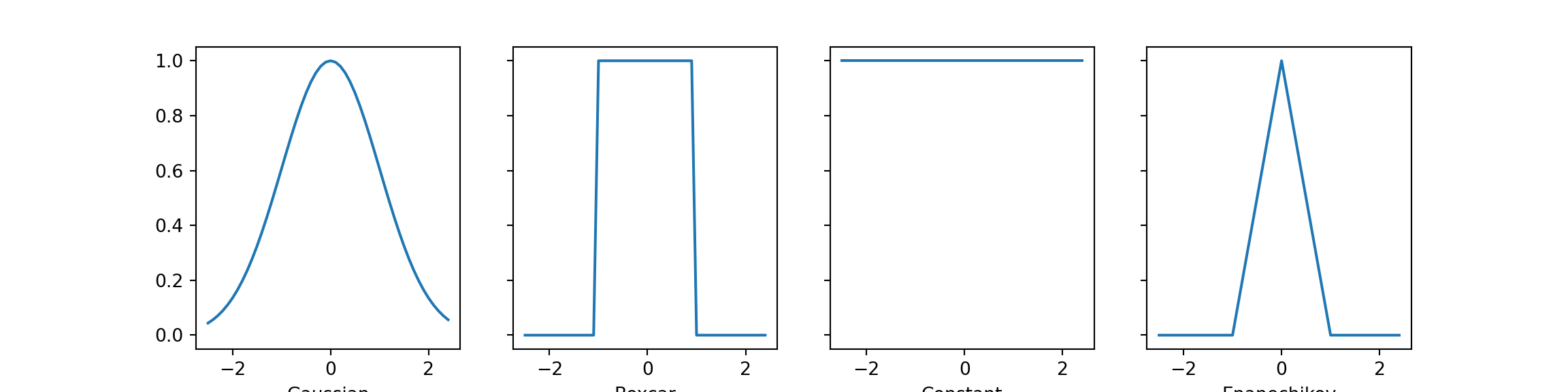
Each of these kernels represents a different way of weighting information based on similarity or distance. In neural networks, this translates to learning how to attend to different parts of the input sequence, but with the flexibility to learn much more complex patterns than these simple mathematical functions.

Now, lets plot the true value of the function and the kernel smoothed value.

Kernel Smoothing using Gaussian Kernel.

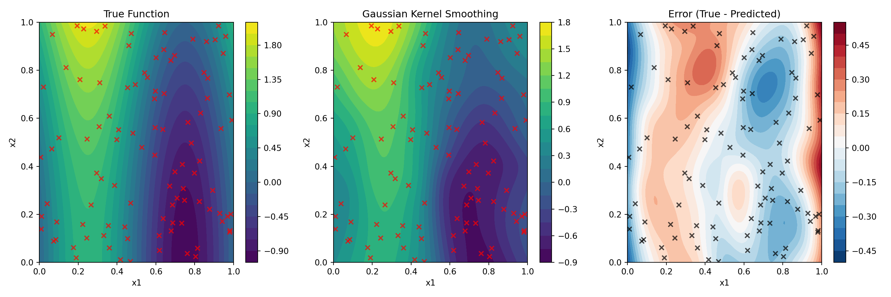
We can see that a relatively simple concept of calculating a prediction by averaging the values of the training data, weighted by the kernel function, can be used to estimate the value of the function at a new point rather well. Clearly, the model is not performing well in the regions where we do not have training data, but it is still able to capture the general shape of the function.

Attention over a Sequence of Words

This mechanism liberates the model from sequential processing. It can process an entire sequence at once, draw connections between distant words, and process information in parallel.

There are two variations of attention that are particularly important: Cross-attention allows a model to weigh the importance of words in an input sequence (like an encoder’s output) when generating a new output sequence (in the decoder). Self-attention allows a model to weigh the importance of different words within a single input sequence.

In self-attention, queries, keys, and values all come from the same sequence. This allows each position in the sequence to attend to all other positions, creating rich representations that capture the complex web of relationships within a single piece of text. When you read a sentence like “The trophy would not fit in the brown suitcase because it was too big,” self-attention helps the model understand that “it” most likely refers to the trophy, not the suitcase, by considering the relationships between all the words simultaneously.

Let’s now consider a sequence of words (or tokens), where each word is represented as a vector (embedding) \[ H = [h_1, h_2, \ldots, h_n] \in \mathbb{R}^{n \times d}. \] Here \(n\) is the length of our sequence to be analyzed. It can be a sentence, a paragraph, or a document. In case of self-attention, the trio of \(Q, K, V\) are all projections of the same input sequence \(H\)

\[ Q = H W_Q, \quad K = H W_K, \quad V = H W_V. \] The projections are done by multiplying the input sequence \(H\) by a learnable parameter matrix \(W_Q, W_K, W_V \in \mathbb{R}^{d \times d_k}\). Thus the resulting \(Q, K, V\) are of dimension \(n \times d_k\). Now, we can calculate the unnormalized attention scores as: \[ s_{ij} = \frac{q_i^\top k_j}{\sqrt{d_k}}, \quad i,j = 1, \ldots, n. \] where \(q_i\) is the \(i\)-th row of \(Q\), \(k_j\) is the \(j\)-th row of \(K\), and \(d_k\) is the dimension of the key vectors. The attention weights are then obtained by normalizing with the softmax function: \[ \alpha_{ij} = \frac{\exp(s_{ij})}{\sum_{l=1}^n \exp(s_{il})}. \] This softmax normalization ensures that attention weights sum to one, creating a proper probability distribution over the input positions. The scaling factor \(1/\sqrt{d_k}\) prevents the dot products from becoming too large, which would push the softmax into regions with extremely small gradients.

The final output is then computed as: \[ o_i = \sum_{j=1}^n \alpha_{ij} v_j. \] where \(o_i\) is the \(i\)-th row of the output.

Notice that instead of using the Gaussian kernel, as we did before, we simply use the dot product. A dot product over a whole sequence is one matrix-matrix multiply, the operation accelerators are built for, and it is smooth in \(Q\) and \(K\), so gradients flow through it. (Smoothness is not the same as stability: unscaled dot products grow with \(d_k\) and saturate the softmax, which is exactly what the \(1/\sqrt{d_k}\) factor is there to prevent.) Non-differentiable attention, trained by reinforcement learning rather than backpropagation, does exist (Mnih et al. 2014), but it is harder to optimize, and the differentiable form has become standard.

The dot product naturally measures the alignment or “similarity” between two vectors. A larger dot product implies the vectors are pointing in a similar direction. When combined with the scaling factor and the softmax function, this simple calculation has proven to be a highly effective way to determine which tokens are most relevant to each other for language processing tasks. It provides a good signal for “unnormalized alignment” before being converted into a probability distribution. In fact, the dot product is a special case of a kernel function. For normalized vectors, the dot product is equivalent to the cosine similarity. \[ Q_i \cdot K_j = \cos(\theta_{ij}) \] where \(\theta_{ij}\) is the angle between the \(i\)-th and \(j\)-th vectors. Squared distance and dot product then carry the same information, \[ \|Q_i - K_j\|^2 = 2 - 2\cos(\theta_{ij}), \] so a large dot product is precisely a small distance. In fact, if \(Q\) and \(K\) are normalized and \(\sigma\) is tuned, the Gaussian kernel becomes almost equivalent to a softmax over dot products. For the specific tasks that attention methods excel at, more complex kernels like the Gaussian kernel haven’t demonstrated a consistent or significant enough improvement in performance to justify their increased computational overhead.

Now instead of calculating norms, we calculate the dot product, and instead of having a bandwidth parameter that needs to be tuned, we have projection matrices \(W_Q, W_K, W_V\), that are learned during training.

For example, let’s consider the following sentence:

“The cat sat on the mat”

A trained attention model will produce a matrix of attention weights. In Figure 23.2 rows and columns are indexed by the distinct word types in the sentence, with the repeated determiner shown once; row \(i\) gives the weights \(\alpha_{ij}\) that word \(i\) places on every word \(j\), and so sums to one. The attention weights are then used to compute the output embeddings.

Figure 23.2: Attention weights for the sentence “The cat sat on the mat”.

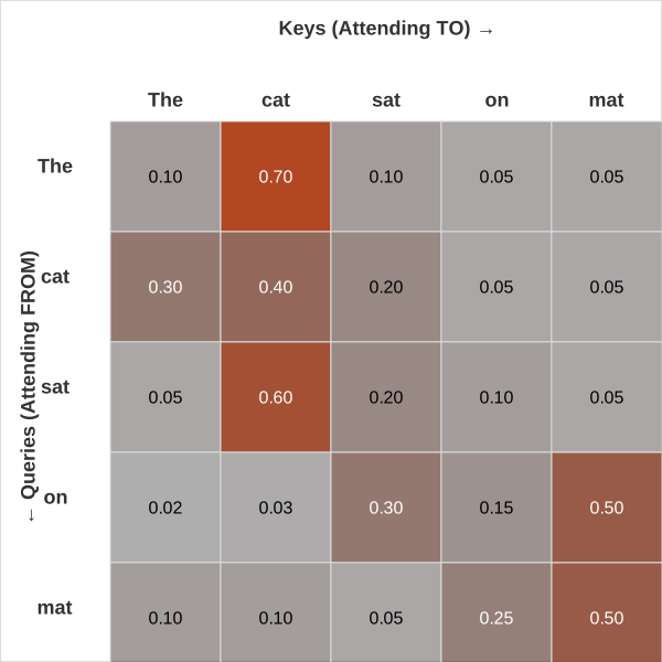
In examining key attention patterns and linguistic insights, we observe several notable relationships. Firstly, the determiner-noun relationship is exemplified by the word “The” showing the strongest attention to its corresponding noun “cat,” with an attention weight of 0.70. This highlights the model’s capability to capture syntactic dependencies between determiners and their head nouns.

Next, we consider subject-predicate dependencies. The verb “sat” demonstrates a strong attention to its subject “cat,” with a weight of 0.60, indicating that the model effectively learns subject-verb relationships, which are central to semantic understanding. Conversely, the attention from “cat” to “sat” is weaker, with a weight of 0.20, illustrating asymmetric attention patterns.

In terms of prepositional phrase structure, the preposition “on” shows a strong attention to its object “mat,” with a weight of 0.50, effectively capturing the prepositional phrase structure. The object “mat” reciprocates with moderate attention to its governing preposition “on,” with a weight of 0.25.

Finally, self-attention patterns reveal that diagonal elements exhibit varying self-attention weights. “mat” and “cat” display higher self-attention weights of 0.50 and 0.40, respectively, suggesting their importance as content words in contrast to function words.

Cross-attention is a variant of attention where the queries come from one sequence (typically the decoder), while the keys and values come from a different sequence (typically the encoder). This is the mechanism that allows translation models to “look back” at the source sentence while generating each word. The unnormalized score \(s_{ij}\) is calculated as: \[ s_{ij} = \frac{q_i^\top k_j}{\sqrt{d_k}}, \quad i = 1, \ldots, n_{\text{decoder}}, \quad j = 1, \ldots, n_{\text{encoder}}, \] where \(q_i\) comes from the decoder’s representation and \(k_j\) comes from the encoder’s representation. This measures how important the \(j\)-th word in the source sequence is for generating the \(i\)-th word in the target sequence. The attention weights are then normalized by the softmax function: \[ \alpha_{ij} = \frac{\exp(s_{ij})}{\sum_{k=1}^{n_{\text{encoder}}} \exp(s_{ik})}. \]

Cross-attention for translation. In sequence-to-sequence models, aligning words between source and target languages is needed to maintain meaning and grammatical structure. Cross-attention addresses this by allowing the model to focus on relevant parts of the source sequence when generating each target word.

The sequence-to-sequence is probably the most commonly used application of language models. Examples include machine translation, text summarization, and text generation from a prompt, question-answering, and chatbots.

Consider a problem of translating ``The cat sleeps’ into French. The encoder will produce a sequence of embeddings for the source sentence, and the decoder will produce a sequence of embeddings for the target sentence. The cross-attention mechanism will use English embeddings as keys and values, and French embeddings as queries. The attention weights will be calculated as shown in Figure 23.3.

Figure 23.3: Cross-attention matrix for the translation of “The cat sleeps” into French.

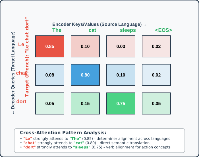
The rows are queries, and are represented by the French decoder tokens [“Le”, “chat”, “dort”]. Columns, which serve as Keys and Values, are represented by the English encoder tokens [“The”, “cat”, “sleeps”, “<EOS>”]. The attention matrix is non-square, with dimensions of 3×4, corresponding to the decoder length and encoder length, respectively.

Key Attention Patterns:

1. Word-by-Word Alignment:
   • The French word “Le” aligns with the English word “The” with an attention weight of 0.85, indicating that determiners align across languages.
   • The French word “chat” aligns with the English word “cat” with an attention weight of 0.80, demonstrating a direct semantic translation.
   • The French word “dort” aligns with the English word “sleeps” with an attention weight of 0.75, showing that verb concepts align.
2. Cross-Linguistic Dependencies:
   • Each French word primarily focuses on its English equivalent, with minimal attention given to unrelated source words. This pattern reflects the model’s ability to learn translation alignments.

Multi-Head Attention: Parallel Perspectives

While single-head attention captures one type of relationship between positions, real language exhibits multiple types of dependencies simultaneously. Consider the sentence “The student who studied hard passed the exam.” We might want to simultaneously track:

• Syntactic relationships (subject-verb agreement between “student” and “passed”)
• Semantic relationships (causal connection between “studied hard” and “passed”)
  
• Coreference relationships (resolution of “who” to “student”)

Multi-head attention addresses this by computing multiple attention functions in parallel, each potentially specializing in different types of relationships:

\[\text{MultiHead}(\mathbf{Q}, \mathbf{K}, \mathbf{V}) = \text{Concat}(\text{head}_1, \ldots, \text{head}_h)\mathbf{W}_O\]

where each head is computed as:

\[\text{head}_i = \text{Attention}(\mathbf{Q}\mathbf{W}_Q^i, \mathbf{K}\mathbf{W}_K^i, \mathbf{V}\mathbf{W}_V^i)\]

The projection matrices \(\mathbf{W}_Q^i, \mathbf{W}_K^i, \mathbf{W}_V^i\) are typically chosen so that \(d_k = d_v = d_{\text{model}}/h\), keeping the total computational cost comparable to single-head attention with full dimensionality.

The final linear projection \(\mathbf{W}_O\) allows the model to learn how to combine information from different heads. This design enables the model to attend to different representation subspaces simultaneously, capturing multiple types of relationships that might be difficult for a single attention head to model.

Positional Information in Attention

Unlike recurrent networks that process sequences step by step, attention is permutation-equivariant: permute the input tokens and the outputs \(o_i\) are permuted the same way, with no output vector changing value. A token’s representation therefore depends on which tokens surround it but never on where it sits, so word order is lost. The property enables parallelization, but it discards positional information essential for language understanding.

The Transformer architecture addresses this through positional encodings that are added to the input embeddings before attention computation. The original formulation uses sinusoidal encodings:

\[\text{PE}(\text{pos}, 2i) = \sin\left(\frac{\text{pos}}{10000^{2i/d_{\text{model}}}}\right)\] \[\text{PE}(\text{pos}, 2i+1) = \cos\left(\frac{\text{pos}}{10000^{2i/d_{\text{model}}}}\right)\]

where \(\text{pos}\) is the position and \(i\) is the dimension. This encoding has several desirable properties:

• Different frequencies allow the model to distinguish positions at different scales
• The sinusoidal structure enables the model to extrapolate to longer sequences than seen during training
• The encoding is deterministic and doesn’t require additional parameters

Alternative approaches include learned positional embeddings or relative position encodings that explicitly model the distance between positions rather than their absolute locations.

Computational Efficiency and Practical Considerations

The quadratic complexity of self-attention has motivated numerous efficiency improvements. Sparse attention patterns restrict which positions can attend to each other, reducing complexity while maintaining representational power. For example, local attention only allows positions to attend within a fixed window, while strided attention creates dilated patterns that maintain long-range connectivity.

Linear attention approximates the full attention matrix with low-rank decompositions or kernel feature maps, cutting the cost from \(O(n^2 d)\) to \(O(n d^2)\), linear rather than quadratic in sequence length. While these methods sacrifice some representational capacity, they enable processing of much longer sequences.

Gradient accumulation, mixed precision training, and gradient checkpointing have become standard practices for training large attention-based models. The first simulates larger batch sizes on limited hardware, the second uses 16-bit floating point for most operations while maintaining 32-bit precision for critical computations, and the third trades recomputation for memory by discarding intermediate activations and regenerating them during the backward pass.

From Attention to Modern Language Models

The attention mechanism’s success stems from its ability to create flexible, context-dependent representations while maintaining computational efficiency through parallelization. This foundation enabled the development of increasingly sophisticated architectures:

• BERT uses bidirectional self-attention encoders for contextual understanding
• GPT employs causal self-attention decoders for autoregressive generation
• T5 combines encoder-decoder architectures for sequence-to-sequence tasks

Each of these models builds on the query-key-value framework, demonstrating its fundamental importance to modern NLP. The attention mechanism’s interpretability—we can visualize attention weights to understand what the model focuses on—provides valuable insights into model behavior and has influenced model design and debugging practices.

The shift from fixed word embeddings to dynamic, context-dependent representations via attention is the key architectural change underlying modern NLP. By weighting different tokens differently for each position, attention captures the long-range dependencies that earlier RNN-based approaches struggled to model.

23.7 Transformer Architecture

The Transformer represents a fundamental shift in neural network architectures for sequential data. Introduced by Vaswani et al. (2017), the Transformer has become the foundation of leading language models, from OpenAI’s GPT series to Google’s Gemini and Meta’s Llama. Beyond text generation, Transformers have proven versatile, finding applications in audio generation, image recognition, protein structure prediction, and game playing.

At its core, text-generative Transformer models perform next-word prediction. Given a text prompt, the model determines the most probable next word. This objective, when scaled to billions of parameters and trained on vast text corpora, produces emergent capabilities.

Self-attention is what lets a Transformer process an entire sequence at once rather than one token at a time. Parallel processing trains efficiently on modern hardware and captures long-range dependencies that recurrent networks handle poorly.

While modern language models like GPT-4 are believed to contain hundreds of billions of parameters, the fundamental architectural principles can be understood through smaller models like GPT-2. The GPT-2 small model, with its 124 million parameters, shares the same core components and principles found in today’s most powerful models, making it an ideal vehicle for understanding the underlying mechanics.

Figure 23.4 shows the schematic representation of a Transformer architecture.

%%{init: {'flowchart': {'wrappingWidth': 130}}}%%
flowchart LR
    I[Input tokens] --> IE[Embedding +<br/>Positional Encoding]
    IE --> E1
    subgraph ENC [Encoder block, x N]
        direction TB
        E1[Multi-Head<br/>Self-Attention] --> E2[Feed-Forward<br/>Network]
    end
    O[Output tokens<br/>shifted right] --> OE[Embedding +<br/>Positional Encoding]
    OE --> D1
    subgraph DEC [Decoder block, x N]
        direction TB
        D1[Masked Multi-Head<br/>Self-Attention] --> D2[Encoder-Decoder<br/>Cross-Attention]
        D2 --> D3[Feed-Forward<br/>Network]
    end
    E2 -- keys, values --> D2
    D3 --> L[Linear + Softmax]
    L --> P[Output<br/>probabilities]

Figure 23.4: Encoder-decoder Transformer. Input tokens are embedded and given positional encodings, then passed through \(N\) encoder blocks of multi-head self-attention and feed-forward layers. Each decoder block applies masked self-attention, then cross-attention over the encoder output, then a feed-forward layer; a linear projection and softmax produce the next-token distribution.

Transformer consists of four fundamental components that work in concert to transform raw text into meaningful predictions. The first step involves converting text to numbers (Tokenizer, Embedding Layer, Positional Encoding). The second step involves the Self-Attention mechanism. The third step involves the Multi-Layer Perceptron (MLP). The final step involves the Output Probabilities. We have covered the first two steps in the previous section. Now we will cover the third step, the Multi-Layer Perceptron. Following the attention mechanism, each token’s representation passes through a position-wise feedforward network. The MLP serves a different purpose than attention: while attention routes information between tokens, the MLP transforms each token’s representation independently.

The MLP consists of two linear transformations with a GELU activation function:

\[\text{MLP}(x) = \text{GELU}(xW_1 + b_1)W_2 + b_2\]

The first transformation expands the dimensionality, allowing the model to use a higher-dimensional space for computation before projecting back to the original size. This expansion provides the representational capacity needed for complex transformations while maintaining consistent dimensions across layers.

After processing through all Transformer blocks, the final step converts the rich contextual representations back into predictions over the vocabulary. This involves two key operations. First, the final layer representations are projected into vocabulary space using a linear transformation:

\[\text{logits} = \text{final\_representations} \cdot W_{\text{output}} + b_{\text{output}}\]

This produces a vector of \(|V|\) values (one for each token in the vocabulary) called logits, representing the model’s raw preferences for each possible next token.

The logits are converted into a probability distribution using the softmax function:

\[P(\text{token}_i) = \frac{\exp(\text{logit}_i)}{\sum_{j=1}^{|\mathcal{V}|} \exp(\text{logit}_j)}\]

This creates a valid probability distribution where all values sum to 1, allowing us to sample the next token based on the model’s learned preferences.

While the three main components form the core of the Transformer, several additional mechanisms enhance stability and performance:

Layer Normalization

Applied twice in each Transformer block (before attention and before the MLP), layer normalization stabilizes training by normalizing activations across the feature dimension:

\[\text{LayerNorm}(x) = \frac{x - \mu}{\sigma} \odot \gamma + \beta\]

where \(\mu\) and \(\sigma\) are the mean and standard deviation computed across the feature dimension, and \(\gamma\) and \(\beta\) are learned scaling and shifting parameters.

Residual Connections

Residual connections create shortcuts that allow gradients to flow directly through the network during training:

\[\text{output} = x + \text{Sublayer}(\text{LayerNorm}(x))\]

These connections are essential for training deep networks, preventing the vanishing gradient problem that would otherwise make it difficult to update parameters in early layers.

Dropout

During training, dropout randomly zeros out a fraction of neuron activations, preventing overfitting and encouraging the model to learn more robust representations. Dropout is typically disabled during inference.

The complete Transformer architecture consists of two main components working in harmony. The encoder stack processes input sequences through multiple layers of multi-head self-attention and position-wise feedforward networks, enhanced with residual connections and layer normalization that help stabilize training. The decoder stack uses masked multi-head self-attention to prevent the model from “cheating” by looking at future tokens during training.

This architecture enabled the development of three distinct families of models, each optimized for different types of tasks. Encoder-only models like BERT excel at understanding tasks such as classification, question answering, and sentiment analysis. They can see the entire input at once, making them particularly good at tasks where understanding context from both directions matters.

Decoder-only models like GPT are particularly good at generation tasks, producing coherent, contextually appropriate text. These models are trained to predict the next token given all the previous tokens in a sequence, which might seem simple but turns out to be incredibly powerful for natural text generation.

Encoder-decoder models like T5 bridge both worlds, excelling at sequence-to-sequence tasks like translation and summarization. The text-to-text approach treats all tasks as text generation problems. Need to translate from English to French? The model learns to generate French text given English input. Want to answer a question? The model generates an answer given a question and context.

23.8 Pretraining at Scale: BERT and Beyond

The availability of powerful architectures raised a key question: how can we best use unlabeled text to learn general-purpose representations? BERT (Bidirectional Encoder Representations from Transformers) (Devlin et al. 2019) introduced a pretraining framework that has become the foundation for modern NLP.

BERT’s key innovation was masked language modeling (MLM), where 15% of tokens are selected for prediction. For each selected token, 80% are replaced with [MASK], 10% with random tokens, and 10% left unchanged. This prevents the model from simply learning to copy tokens when they’re not masked. The loss function only considers predictions for masked positions:

\[\mathcal{L}_{\text{MLM}} = -\sum_{m \in \mathcal{M}} \log P(x_m \mid \mathbf{x}_{\backslash \mathcal{M}})\]

BERT combines MLM with next sentence prediction (NSP), which trains the model to understand relationships between sentence pairs. Training examples contain 50% consecutive sentences and 50% randomly paired sentences. The input representation concatenates both sentences with special tokens and segment embeddings to distinguish between them.

The scale of BERT pretraining represents a quantum leap from earlier approaches. The original BERT models were trained on a combination of BookCorpus (800 million words from over 11,000 books) and English Wikipedia (2,500 million words). This massive dataset enables the model to see diverse writing styles, topics, and linguistic phenomena. The preprocessing pipeline removes duplicate paragraphs, filters very short or very long sentences, and maintains document boundaries to ensure coherent sentence pairs for NSP.

BERT Architecture and Training Details

To understand BERT’s architectural significance, it’s helpful to compare it with its predecessors ELMo and GPT, which represent different approaches to contextual representation learning:

Figure 23.5: Comparison of ELMo, GPT, and BERT architectures.

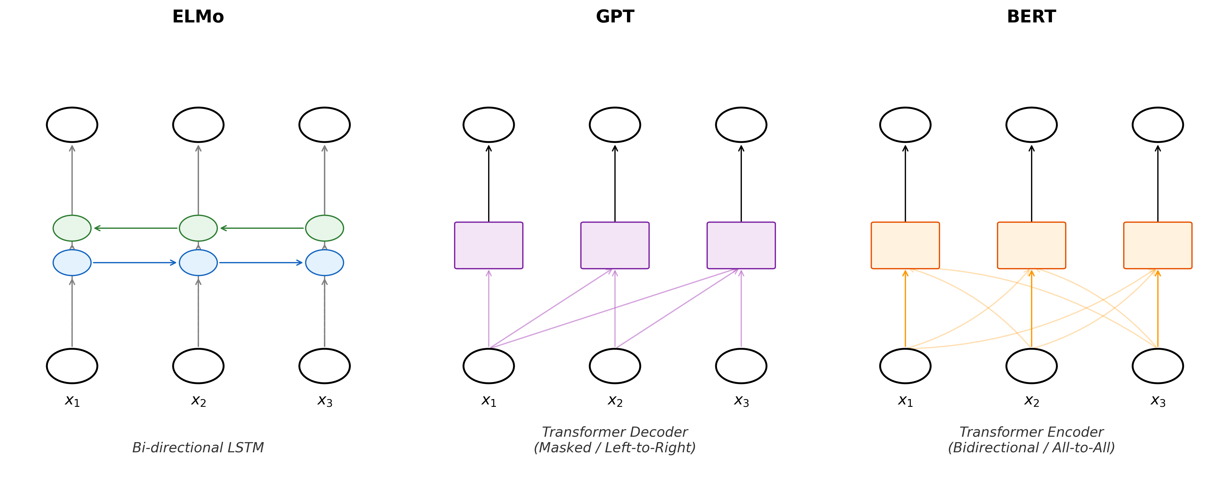
ELMo uses bidirectional LSTMs with task-specific architectures, requiring custom model design for each application. GPT employs a unidirectional Transformer decoder that processes text left-to-right, making it task-agnostic but unable to see future context. BERT combines the best of both: bidirectional context understanding through Transformer encoders with minimal task-specific modifications (just an output layer). BERT comes in two main configurations that balance model capacity with computational requirements:

BERT configurations and parameters.

Model	Transformer Layers	Hidden Dimensions	Attention Heads	Parameters
BERT-Base	12	768	12	110M
BERT-Large	24	1024	16	340M

Both models use a vocabulary of 30,000 WordPiece tokens, learned using a data-driven tokenization algorithm similar to BPE. The maximum sequence length is 512 tokens, though most pretraining uses sequences of 128 tokens to improve efficiency, with only the final 10% of training using full-length sequences.

The pretraining procedure involves several techniques to stabilize and accelerate training:

1. Warm-up Learning Rate: The learning rate increases linearly for the first 10,000 steps to \(10^{-4}\), then decreases linearly. This warm-up prevents large gradients early in training when the model is randomly initialized.
2. Large Effective Batches: BERT trains on batches of 256 sequences, 128,000 tokens per update. Hardware that cannot hold a batch this large can accumulate gradients over several forward passes before updating the weights.
3. Mixed Precision Training: Using 16-bit floating point for most computations while maintaining 32-bit master weights speeds up training significantly on modern GPUs.

Data Preparation for BERT Pretraining

The data preparation pipeline for BERT is surprisingly complex. Starting with raw text, the process involves:

graph LR
    A[Raw Text] --> B[Document Segmentation]
    B --> C[Sentence Segmentation]
    C --> D[WordPiece Tokenization]
    D --> E[Creating Training Examples]
    E --> F[Creating TFRecord Files]

In the document segmentation stage, text is split into documents, maintaining natural boundaries. For books, this means chapter boundaries; for Wikipedia, article boundaries. The next stage is sentence segmentation, where each document is split into sentences using heuristic rules. Typically, this involves identifying periods followed by whitespace and capital letters, while accounting for exceptions such as abbreviations.

Following sentence segmentation, the text undergoes WordPiece tokenization. This process uses a learned WordPiece vocabulary to break text into subword units, ensuring that unknown words can be represented as sequences of known subwords. Special handling is applied to mark the beginning of words.

Once tokenized, the data are organized into training examples. For each example, a target sequence length is sampled from a geometric distribution to introduce variability. Sentences are packed together until the target length is reached. For the next sentence prediction (NSP) task, half of the examples use the actual next segment, while the other half use a randomly selected segment. Masked language modeling (MLM) is applied by masking 15% of tokens, following the 80/10/10 strategy: 80% of the time the token is replaced with [MASK], 10% with a random token, and 10% left unchanged. Special tokens such as [CLS] at the beginning and [SEP] between segments are added, and segment embeddings are created (0 for the first segment, 1 for the second). Sequences are padded to a fixed length using [PAD] tokens.

Finally, the prepared examples are serialized into TFRecord files for efficient input/output during training. Examples are grouped by sequence length to minimize the amount of padding required.

The democratization of pretraining through libraries like Hugging Face Transformers has made it possible for smaller organizations to apply these techniques, either by fine-tuning existing models or pretraining specialized models for their domains.

23.9 Transfer Learning and Downstream Applications

The power of pretrained models lies in their transferability. The landscape of NLP applications can be broadly categorized into two fundamental types based on their input structure and prediction granularity. Sequence-level tasks operate on entire text sequences, producing a single output per input sequence or sequence pair. Token-level tasks make predictions for individual tokens within sequences, such as named entity recognition that identifies person names, locations, and organizations. A third family, sequence-to-sequence tasks, generates a new sequence from the input. Figure 23.6 maps representations to architectures to tasks.

%%{init: {'themeCSS': '.mermaid svg { background-color: #f8f9fa; }'}}%%
graph TB
    subgraph P [Pretrained Representations]
        P1[Word2Vec/GloVe]
        P2[BERT/RoBERTa]
        P3[GPT/T5]
    end

    subgraph A [Architectures]
        A1[MLPs]
        A2[CNNs]
        A3[RNNs]
        A4[Transformers]
        A5[Attention]
    end

    subgraph S [Sequence-Level Tasks]
        S1[Sentiment Analysis]
        S2[Text Classification]
        S3[Natural Language Inference]
        S4[Semantic Similarity]
    end

    subgraph T [Token-Level Tasks]
        T1[Named Entity Recognition]
        T2[Part-of-Speech Tagging]
        T3[Question Answering]
    end

    subgraph G [Sequence-to-Sequence Tasks]
        G1[Machine Translation]
        G2[Text Summarization]
    end

    P1 --> A1
    P1 --> A2
    P1 --> A3
    P2 --> A4
    P2 --> A5
    P3 --> A4

    A1 --> S1
    A1 --> S3
    A2 --> S1
    A2 --> S2
    A3 --> S1
    A3 --> S3
    A3 --> T2
    A4 --> S2
    A4 --> S3
    A4 --> S4
    A4 --> T1
    A4 --> T2
    A4 --> T3
    A4 --> G1
    A4 --> G2
    A5 --> S3
    A5 --> S4
    A5 --> T3

Figure 23.6: Which pretrained representations feed which architectures, and which architectures serve which class of task.

For sentiment analysis, we add a linear layer on top of the [CLS] token representation and fine-tune on labeled data. Popular datasets include IMDb movie reviews (50K examples) and Stanford Sentiment Treebank (11,855 sentences). Modern models can capture nuanced semantic relationships that traditional lexicon-based approaches miss. For instance, the phrase “not bad” expresses mild approval despite containing the negative word “bad,” while “insanely good” uses typically negative intensity (“insanely”) to convey strong positive sentiment. Fine-tuning typically requires only 2-4 epochs, demonstrating the effectiveness of transfer learning.

Natural language inference (NLI) determines logical relationships between premise and hypothesis sentences. The Stanford Natural Language Inference corpus contains 570,000 sentence pairs labeled as entailment, contradiction, or neutral. For BERT-based NLI, we concatenate premise and hypothesis with [SEP] tokens and classify using the [CLS] representation. Because both sentences occupy a single input sequence, self-attention can link a word in the hypothesis directly to the word in the premise that supports or contradicts it.

Token-level tasks like named entity recognition classify each token independently. Common datasets include CoNLL-2003 (English and German entities) and OntoNotes 5.0 (18 entity types). The BIO tagging scheme marks entity boundaries: B-PER for beginning of person names, I-PER for inside, and O for outside any entity. For example, in “Apple Inc. was founded by Steve Jobs”, “Apple” would be tagged B-ORG, “Inc.” as I-ORG, “Steve” as B-PER, and “Jobs” as I-PER.

Question answering presents unique challenges. The SQuAD dataset contains 100,000+ questions where answers are text spans from Wikipedia articles. BERT approaches this by predicting start and end positions independently, with the final answer span selected to maximize the product of start and end probabilities subject to length constraints. For a question like “Who founded Apple?”, the model identifies the span “Steve Jobs” in the context passage.

23.10 Model Compression and Efficiency

While large pretrained models achieve impressive performance, their computational requirements limit deployment. Knowledge distillation trains a small “student” model to mimic a large “teacher” model through a combined loss:

\[\mathcal{L}_{\text{distill}} = \alpha \mathcal{L}_{\text{task}} + (1-\alpha) \text{KL}(p_{\text{teacher}} \| p_{\text{student}})\]

DistilBERT (Sanh et al. 2019) achieves 97% of BERT’s performance with 40% fewer parameters and 60% faster inference. Quantization reduces numerical precision from 32-bit to 8-bit or even lower, while pruning removes connections below a magnitude threshold. These techniques can reduce model size by an order of magnitude with minimal performance degradation.

23.11 Theoretical Perspectives and Future Directions

The success of language models connects to several theoretical frameworks. Transformers are universal approximators for sequence-to-sequence functions: with sufficient capacity and appropriate positional encodings, they can approximate any continuous sequence-to-sequence function on a compact domain to arbitrary precision (Yun et al. 2020). The self-attention mechanism provides an inductive bias well-suited to capturing long-range dependencies.

Despite having hundreds of millions of parameters, these models generalize well. This connects to implicit regularization in overparameterized models, where gradient descent dynamics bias toward solutions with good generalization properties. Language models automatically learn hierarchical features: early layers capture syntax and morphology, middle layers semantic relationships, and later layers task-specific abstractions.

Yet significant challenges remain. Models struggle with compositional generalization: understanding “red car” and “blue house” doesn’t guarantee understanding “red house” if that combination is rare in training. The sample efficiency gap is real: a child hears on the order of 100 million words before mastering basic grammar, while BERT was trained on 3.3 billion and models since on hundreds of billions, suggesting fundamental differences between neural network optimization and human language acquisition.

Interpretability poses ongoing challenges. While attention visualizations provide some insights, we lack principled methods for understanding representations distributed across dozens of layers and hundreds of attention heads. Future directions include multimodal understanding (integrating text with vision and speech), more efficient architectures that maintain performance while reducing computational requirements, and developing theoretical frameworks to predict and understand model behavior.

23.12 Conclusion

The journey from symbolic manipulation to neural language understanding represents a major success of modern artificial intelligence. By reconceptualizing language as geometry in high-dimensional spaces, using self-supervision at scale, and developing architectural innovations like transformers, the field has achieved strong capabilities.

The mathematical frameworks developed, from distributional semantics to attention mechanisms, provide not just engineering tools but lenses through which to examine fundamental questions about meaning and understanding. As these systems become more capable and widely deployed, understanding their theoretical foundations, practical limitations, and societal implications becomes ever more critical.

The techniques discussed in this chapter—word embeddings, contextual representations, pretraining, and fine-tuning—form the foundation of modern NLP systems. Despite impressive engineering achievements, true language understanding remains elusive. The rapid progress offers both tremendous opportunities and sobering responsibilities.

Exercises

Pen-and-Pencil

Exercise 23.1 (Tokenization) For the sentence: “The quick brown fox jumps over the lazy dog.”

1. Tokenize using whitespace splitting. How many tokens?
2. What are the limitations of whitespace tokenization?
3. Using BPE-style subword tokenization, how might “jumping” be tokenized if “jump” and “ing” are in the vocabulary?
4. Why do GPT models use byte-pair encoding rather than word-level tokenization?

Exercise 23.2 (Word Embeddings) Given pre-trained word vectors:

• king = [0.5, 0.8, 0.3, 0.2]
• queen = [0.5, 0.7, 0.35, 0.9]
• man = [0.4, 0.9, 0.2, 0.1]
• woman = [0.4, 0.8, 0.25, 0.8]

1. Calculate the cosine similarity between “king” and “queen”.
2. Verify the famous analogy: king - man + woman \(\approx\) queen
3. What does this suggest about the embedding space?
4. What are limitations of static word embeddings like Word2Vec?

Exercise 23.3 (Attention Mechanism) Consider a simple attention mechanism with:

• Query: q = [1, 0]
• Keys: K = [[1, 0], [0, 1], [1, 1]]
• Values: V = [[10], [20], [30]]

Using scaled dot-product attention (without the scaling factor for simplicity):

1. Calculate the attention scores (K q).
2. Apply softmax to get attention weights.
3. Compute the weighted sum of values.
4. What does this attention mechanism “attend to”?

Exercise 23.4 (Transformer Architecture) In a Transformer encoder:

1. What are the three components of the (self-)attention mechanism? (Hint: Q, K, V)
2. If we have 8 attention heads with d_model = 512, what is the dimension of each head?
3. What is the purpose of positional encoding?
4. Why is layer normalization used after each sub-layer?

Exercise 23.5 (True/False: NLP)  

1. In self-attention, each position can attend to all other positions simultaneously.

2. RNNs process sequences faster than Transformers because they don’t compute attention.

3. BERT uses both left and right context when encoding each token.

4. The softmax in attention ensures attention weights sum to 1.

5. Transformers can handle variable-length sequences without modification.

Exercise 23.6 (Downstream Heads: BIO Tagging and Answer Spans) Chapter 23 describes token-level downstream tasks built on pretrained representations. Two of them turn per-token outputs into structured predictions: named entity recognition via BIO tags, and extractive question answering, which predicts a start and an end position and returns the span maximizing the product of start and end probabilities subject to a length limit.

1. For the sentence “Steve Jobs founded Apple Inc in California” (7 tokens), with entities PER = “Steve Jobs”, ORG = “Apple Inc”, LOC = “California”, write the BIO tag of each token, following Chapter 23 (B- begins an entity, I- continues it, O is outside any entity).

2. For the question “Who founded Apple?” over the passage “Apple was founded by Steve Jobs in 1976” (8 tokens), a QA head outputs the unnormalized start scores \((1, 1, 1, 1, 5, 3, 1, 1)\) and end scores \((1, 1, 1, 1, 3, 4, 1, 5)\) over the tokens. Normalize each with a softmax to get \(P_{\text{start}}\) and \(P_{\text{end}}\). Report \(\arg\max P_{\text{start}}\) and \(\arg\max P_{\text{end}}\) separately, and the span obtained by naively combining the two independent argmaxes. Then, per Chapter 23, select the span \((i, j)\) with \(i \le j\) maximizing \(P_{\text{start}}(i)\,P_{\text{end}}(j)\) subject to a maximum length of 3 tokens (\(j - i + 1 \le 3\)), searching all valid pairs.

3. Compare the naive combination with the length-constrained joint search. Which one recovers “Steve Jobs”, the answer that Chapter 23’s own example names? Why did the constraint matter?

Computing

Exercise 23.7 (Skip-Gram with Negative Sampling) Consider a toy corpus of sixteen three-word “sentences” drawn from two unrelated themes, royalty and pets:

1. Build the vocabulary and, treating each three-word sentence as its own context window (every word is a context word for every other word in the same sentence), construct the list of (center, context) index pairs used for training. Report the vocabulary size and the number of training pairs.

2. Implement skip-gram with negative sampling (Chapter 23) from scratch: a center-word embedding matrix and a context-word embedding matrix, each with one \(d=8\) dimensional row per vocabulary word, a sigmoid function, and the noise distribution \(P_n(w) \propto f(w)^{3/4}\) built from the unigram counts \(f(w)\). Run manual stochastic gradient descent for 400 epochs with \(K=8\) negative samples per positive pair and a learning rate that decays linearly over training, printing the average per-pair loss every 100 epochs. Confirm the loss decreases.

3. Using the trained center embeddings, compute the cosine similarity for the two within-theme pairs (king, queen) and (dog, cat), and for the four cross-theme pairs (king, dog), (king, cat), (queen, dog), (queen, cat). Does the model separate the two themes, even though it was never told they exist?

Exercise 23.8 (GloVe from Global Co-occurrence Counts) While skip-gram slides a window over sentences, GloVe (Chapter 23) fits word vectors directly to global co-occurrence counts. Its motivating observation is that ratios of co-occurrence probabilities carry meaning: \(\prob{\text{solid} \mid \text{ice}}/\prob{\text{solid} \mid \text{steam}}\) is large, \(\prob{\text{gas} \mid \text{ice}}/\prob{\text{gas} \mid \text{steam}}\) is small, and \(\prob{\text{water} \mid \text{ice}}/\prob{\text{water} \mid \text{steam}}\) is near 1.

Work over the five-word vocabulary ["gas", "ice", "solid", "steam", "water"] with symmetric co-occurrence counts ice-steam 3, ice-solid 9, ice-gas 1, ice-water 5, steam-solid 1, steam-gas 9, steam-water 5, solid-gas 1, solid-water 3, and gas-water 3 (all unlisted pairs 0).

1. Build the symmetric co-occurrence matrix \(X\) from counts. Using \(\prob{w_t \mid w_g} = X_{g,t}/\sum_k X_{g,k}\), compute the three ratios above. Do they reproduce the large / small / near-one pattern Chapter 23 describes?

2. Implement the GloVe loss from Chapter 23, \[\mathcal{L}_{\text{GloVe}} = \sum_{i,j} h(X_{ij})\left(\mathbf{v}_i^\top \mathbf{u}_j + b_i + c_j - \log X_{ij}\right)^2,\] with weighting \(h(x) = (x/x_{\max})^{\alpha}\) for \(x < x_{\max}\) and \(1\) otherwise. Because these toy counts are small, use \(x_{\max} = 5\) and \(\alpha = 0.75\) (the chapter’s \(x_{\max} = 100\) is tuned for a billion-word corpus). Initialize \(\mathbf{v}_i, \mathbf{u}_j \in \mathbb{R}^3\) with np.random.seed(26) and \(b_i = c_j = 0\), then run gradient descent over the pairs with \(X_{ij} > 0\) for 800 epochs, printing the average weighted squared error periodically. Confirm it decreases.

3. Using \(\mathbf{v}_i + \mathbf{u}_i\) as word \(i\)’s embedding, compute the cosine similarities between (ice, solid), (steam, solid), (ice, gas), and (steam, gas). Does the trained geometry recover the ratio asymmetry: ice aligned with solid, steam aligned with gas?

Exercise 23.9 (Self-Attention from Scratch) Four tokens, “dog”, “puppy”, “car”, “vehicle”, are embedded by hand (not learned) in \(\mathbb{R}^3\) using three features: how strongly the word denotes an animal, a filler feature that carries no information about that distinction, and how strongly the word denotes a vehicle.

The projection matrices are fixed (not learned), so the whole computation can be checked by hand: \[ W_Q = W_K = \begin{bmatrix} 1 & 0 \\ 0 & 0 \\ 0 & 1 \end{bmatrix}, \qquad W_V = \begin{bmatrix} 0 & 1 \\ 1 & 1 \\ 1 & 0 \end{bmatrix}. \]

1. Form \(Q = XW_Q\), \(K = XW_K\), \(V = XW_V\) in numpy. What do \(W_Q\) and \(W_K\) do to the middle (filler) feature of \(X\)?

2. Compute the scaled scores \(QK^\top/\sqrt{d_k}\) and the attention weight matrix \(\alpha = \text{softmax}(QK^\top/\sqrt{d_k})\), with the softmax taken row-wise as in Chapter 23. Verify numerically that every row of \(\alpha\) sums to 1.

3. For each token, report which other token it attends to most strongly. Does the attention pattern recover the fact that “dog” and “puppy” are related, and separately that “car” and “vehicle” are related, given that this was only implicit in \(X\)?

Exercise 23.10 (Byte Pair Encoding from Scratch) Chapter 23 introduces BPE on the word frequencies {“fast”: 4, “faster”: 3, “tall”: 5, “taller”: 4} and predicts that the first merges will be “t” + “a” \(\rightarrow\) “ta”, then “ta” + “l” \(\rightarrow\) “tal”. This exercise implements BPE and checks that prediction against real merge counts.

Each word starts out as a tuple of single-character symbols followed by an end-of-word marker </w>, tagged with its corpus frequency.

1. Write get_pair_counts(vocab), returning for every adjacent symbol pair the total frequency (summed over words) with which it occurs, and merge_pair(pair, vocab), which replaces every adjacent occurrence of pair with the merged symbol throughout vocab. Using these two functions, run 8 rounds of “find the most frequent pair, merge it,” printing the merge and its count at each step. Do the first three merges match the chapter’s prediction?

2. Print vocab after the 8 merges. How many merges does it take before “fast” and “tall” each become a single symbol (plus </w>)?

3. Write bpe_tokenize(word, merges), which applies the learned merges, in order, to a new word, and use it to tokenize the unseen words “fastest” and “tallest”. Why does the stem survive as one token while the superlative suffix does not, and what does this predict for a word like “smartest” if training data only ever showed the comparative “smarter”?

Exercise 23.11 (Masked Language Modeling from Scratch) Chapter 23 introduces BERT’s masked language modeling (MLM): 15% of token positions are selected for prediction, and each selected position is corrupted by the 80/10/10 recipe (80% replaced with [MASK], 10% replaced with a random word, 10% left unchanged). The loss \[\mathcal{L}_{\text{MLM}} = -\sum_{m \in \mathcal{M}} \log P(x_m \mid \mathbf{x}_{\backslash \mathcal{M}})\] is evaluated only at the selected positions \(\mathcal{M}\). This exercise implements the masking and a simplified MLM objective on a toy corpus of twelve five-word sentences over a 16-word vocabulary.

1. Implement BERT’s masking from Chapter 23: visit every token position, select it with probability 0.15, and for each selected position draw a corruption type with probabilities 0.8 (replace with [MASK]), 0.1 (replace with a random vocabulary word), 0.1 (leave unchanged). With np.random.seed(26), report how many of the 60 positions are selected and the count of each corruption type, recording for every selected position the true word (needed for the loss).

2. Implement a simplified MLM loss. Give each vocabulary word and [MASK] a trainable \(d = 8\) embedding. For a selected position \(m\), form the context vector as the average of the (corrupted) embeddings at the other positions of the same sentence, project it to logits over the vocabulary with a trainable linear layer, and compute cross-entropy \(-\log P(x_m \mid \mathbf{x}_{\backslash \mathcal{M}})\) only at the selected positions. Run gradient descent for 400 epochs, printing the average loss periodically. Confirm it decreases.

3. One selected position falls in the 10% “leave unchanged” branch: its input token is not altered, yet the loss is still computed there. Explain why BERT keeps these positions in the loss instead of scoring only positions where the input was actually replaced.

Bahdanau, Dzmitry, Kyunghyun Cho, and Yoshua Bengio. 2014. “Neural Machine Translation by Jointly Learning to Align and Translate.” arXiv. https://arxiv.org/abs/1409.0473.

Bojanowski, Piotr, Edouard Grave, Armand Joulin, and Tomas Mikolov. 2017. “Enriching Word Vectors with Subword Information.” Transactions of the Association for Computational Linguistics 5: 135–46.

Devlin, Jacob, Ming-Wei Chang, Kenton Lee, and Kristina Toutanova. 2019. “BERT: Pre-training of Deep Bidirectional Transformers for Language Understanding.” In Proceedings of the 2019 Conference of the North American Chapter of the Association for Computational Linguistics: Human Language Technologies, Volume 1 (Long and Short Papers), 4171–86. Minneapolis, Minnesota: Association for Computational Linguistics.

Firth, John Rupert. 1957. “A Synopsis of Linguistic Theory, 1930–1955.” In Studies in Linguistic Analysis, 1–32. Oxford: Blackwell.

Levy, Omer, and Yoav Goldberg. 2014. “Neural Word Embedding as Implicit Matrix Factorization.” In Advances in Neural Information Processing Systems, 27:2177–85.

Mikolov, Tomas, Kai Chen, Greg Corrado, and Jeffrey Dean. 2013. “Efficient Estimation of Word Representations in Vector Space.” arXiv. https://arxiv.org/abs/1301.3781.

Mnih, Volodymyr, Nicolas Heess, Alex Graves, and Koray Kavukcuoglu. 2014. “Recurrent Models of Visual Attention.” In Advances in Neural Information Processing Systems, 27:2204–12.

Pennington, Jeffrey, Richard Socher, and Christopher D. Manning. 2014. “GloVe: Global Vectors for Word Representation.” In Proceedings of the 2014 Conference on Empirical Methods in Natural Language Processing (EMNLP), 1532–43. Doha, Qatar: Association for Computational Linguistics.

Sanh, Victor, Lysandre Debut, Julien Chaumond, and Thomas Wolf. 2019. “DistilBERT, a Distilled Version of BERT: Smaller, Faster, Cheaper and Lighter.” arXiv Preprint arXiv:1910.01108. https://arxiv.org/abs/1910.01108.

Vaswani, Ashish, Noam Shazeer, Niki Parmar, Jakob Uszkoreit, Llion Jones, Aidan N. Gomez, Łukasz Kaiser, and Illia Polosukhin. 2017. “Attention Is All You Need.” Advances in Neural Information Processing Systems 30: 5998–6008.

Yun, Chulhee, Srinadh Bhojanapalli, Ananda Theertha Rawat, Sashank J. Reddi, and Sanjiv Kumar. 2020. “Are Transformers Universal Approximators of Sequence-to-Sequence Functions?” In International Conference on Learning Representations (ICLR). https://arxiv.org/abs/1912.10077.