data(iris)
y = iris$Petal.Length20 Gradient Descent
“Elegance is found in reducing parameters, not multiplying them.”—Boris Polyak
How does a neural network with millions of parameters learn the right values? Classical statistical models rely on second-order optimization: least squares for linear regression and Newton-type methods like Broyden-Fletcher-Goldfarb-Shanno (BFGS) for generalized linear models. These algorithms use curvature information (the Hessian matrix) to take efficient steps toward the optimum.
However, second-order optimization algorithms do not scale well to deep learning models. When a model has millions or billions of parameters, computing and storing the Hessian matrix becomes prohibitive from both computational and memory standpoints. Instead, first-order gradient descent methods, which require only gradient information, are the workhorses for training deep neural networks.
This chapter unifies a theme that already appeared earlier: in Chapter 11 we framed estimation as likelihood maximization and showed how the negative log-likelihood becomes a loss. In Chapter 8 we used the same idea computationally to fit Gaussian process hyperparameters by maximizing a marginal likelihood (via optim). Here we make the optimization mechanics explicit and reusable.
Given a parametric model \(f_{\theta}(x)\), the problem of parameter estimation (when the likelihood belongs to the exponential family) is an optimization problem: \[ \min_{\theta} l(\theta) := -\dfrac{1}{n} \sum_{i=1}^n \log p(y_i \mid x_i, \theta), \] where \(l\) is the negative log-likelihood of a sample (equivalently, \(l(\theta)=-\ell(\theta)\) up to scaling, with \(\ell(\theta)=\log L(\theta)\) as in Chapter 11), and \(\theta\) is the vector of parameters. The gradient descent method is an iterative algorithm that starts with an initial guess \(\theta^{0}\) and then updates the parameter vector \(\theta\) at each iteration \(t\) as follows: \[ \theta^{t+1} = \theta^t - \alpha_t \nabla l(\theta^t). \] Here \[ \nabla l(\theta^t) = \left(\frac{\partial l}{\partial \theta_0}, \ldots,\frac{\partial l}{\partial \theta_p}\right), \] is the gradient of the loss function with respect to the parameters at iteration \(t\).
This algorithm is based on the simple fact that a function value decreases in the direction of the negative gradient, at least locally. This fact follows from the definition of the gradient, which is the vector of partial derivatives of the function with respect to its parameters. The gradient points in the direction of the steepest ascent, and thus the negative gradient points in the direction of the steepest descent. It is easy to see in the figure below, where the function \(l(x)\) is shown in blue and the gradient at the point \(x_0\) is shown in red. The negative gradient points in the direction of the steepest descent, which is the direction we want to go to minimize the function. We can easily see it in a one-dimensional case. The derivative is defined as \[ l'(\theta) = \lim_{h \to 0} \frac{l(\theta+h) - l(\theta)}{h}. \] The derivative is the slope of the tangent line to the function at the point \(\theta\). The derivative is positive, when \(l(\theta+h) > l(\theta)\) for small \(h > 0\), then the function is increasing at that point, and if it is negative, then the function is decreasing at that point. Thus, we can use the negative derivative to find the direction of the steepest descent.
For the derivative (or gradient in the multivariate case) to be defined, the function \(l(\theta)\) must be continuous and smooth at the point \(\theta\). In practice, this means that the function must not have any sharp corners or discontinuities. For example, \(f(\theta) = |\theta|\) has a sharp corner at zero, with a derivative of \(+1\) for \(\theta > 0\) and \(-1\) for \(\theta < 0\). At zero itself, the derivative is undefined. This is called a non-differentiable point. Another example is the sign function \(f(\theta) = \text{sign}(\theta)\), which has a discontinuity at zero.
This matters for deep learning because the popular ReLU activation function \(\max(0, x)\) has a non-differentiable point at zero. Gradient descent, despite operating on these non-smooth loss surfaces, remains the workhorse for training deep neural networks. In practice, this works because: (1) the probability of landing exactly at a non-differentiable point is zero for continuous distributions, and (2) subgradients provide valid descent directions even at kinks.
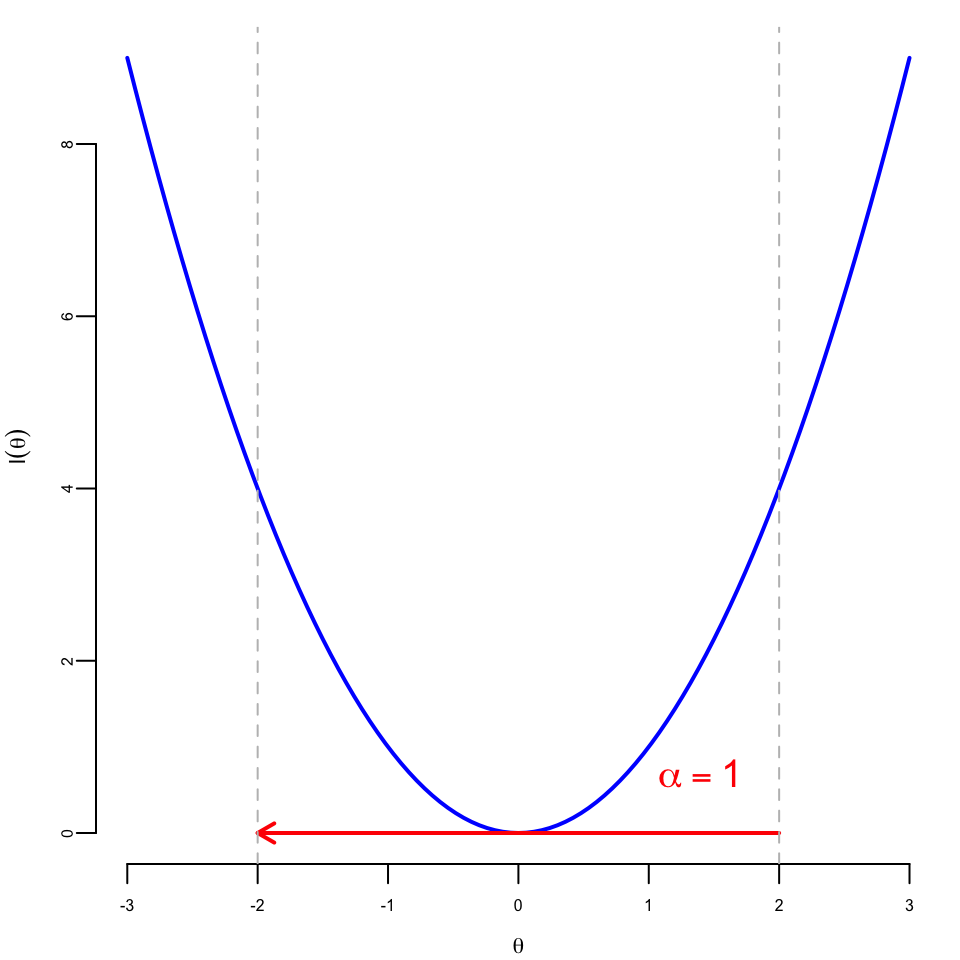
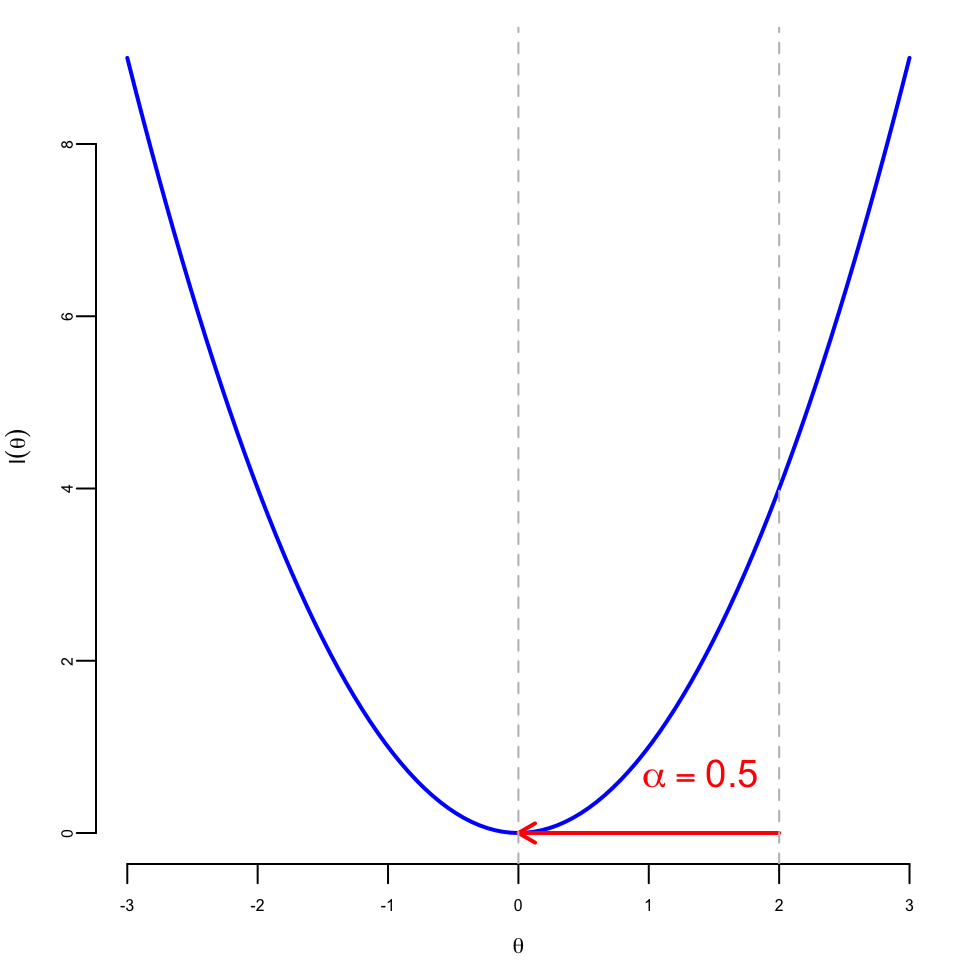
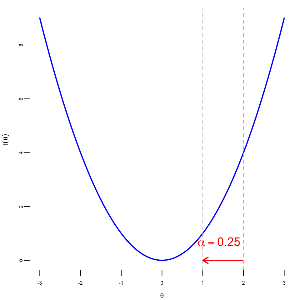
The second component is the learning rate \(\alpha_t\), a positive scalar controlling the step size. If the learning rate is too small, convergence is slow; if too large, the algorithm may diverge or oscillate. Figure 20.1 shows this effect: when \(\alpha = 0.5\), the algorithm converges in one step from \(\theta_0 = 2\); when \(\alpha = 0.25\), it converges more slowly; when \(\alpha = 1\), it overshoots the minimum.
In practice, the learning rate is often set to a small value, such as \(0.01\) or \(0.001\), and then adjusted during the training process. There are several techniques for adjusting the learning rate, such as learning rate decay, where the learning rate is reduced by a factor at each epoch, or adaptive learning rates, where the learning rate is adjusted based on the gradient of the loss function.
20.1 Deep Learning and Least Squares
The deep learning model approximates the relation between inputs \(x\) and outputs \(y\) using a non-linear function \(f_{\theta}(x)\), where \(\theta\) is a vector of parameters. The goal is to find the optimal value of \(\theta\) that minimizes the negative log-likelihood (loss function), given a training dataset \(D = \{x_i,y_i\}_{i=1}^n\). The loss function is a measure of discrepancy between the true value of \(y\) and the predicted value \(f_{\theta}(x)\) \[ l(\theta) = - \sum_{i=1}^n \log p(y_i \mid x_i, \theta), \] where \(p(y_i \mid x_i, \theta)\) is the conditional likelihood of \(y_i\) given \(x_i\) and \(\theta\). In the case of regression, we have \[ y_i = f_{\theta}(x_i) + \epsilon, ~ \epsilon \sim N(0,\sigma^2), \] The loss function is then (dropping the constant term \(-n\log(\sigma\sqrt{2\pi})\)): \[ l(\theta) = - \sum_{i=1}^n \log p(y_i \mid x_i, \theta) \propto \sum_{i=1}^n (y_i - f_{\theta}(x_i))^2, \]
Now, let’s demonstrate the gradient descent algorithm on a simple example of linear regression using the iris dataset.
Example 20.1 (Linear Regression) Linear regression can be viewed as a degenerate neural network: a single layer with no hidden units and an identity activation function. The insight of deep learning is that using deep and narrow architectures (multiple layers with fewer units per layer) enables learning complex, hierarchical representations.
Let’s fit a linear regression model to the iris dataset using gradient descent. We use \(y =\) Petal.Length as the response variable and \(x =\) Petal.Width as the predictor. The model is \[
y_i = \theta_0 + \theta_1 x_i + \epsilon_i,
\] or in matrix form: \[
y = X \theta + \epsilon,
\] where \(\epsilon_i \sim N(0, \sigma^2)\), \(X = [1 ~ x]\) is the design matrix with first column being all ones.
The negative log-likelihood function for the linear regression model is: \[ l(\theta) = \sum_{i=1}^n (y_i - \theta_0 - \theta_1 x_i)^2. \] The gradient is then: \[ \nabla l(\theta) = -2 \sum_{i=1}^n (y_i - \theta_0 - \theta_1 x_i) \begin{pmatrix} 1 \\ x_i \end{pmatrix}. \] In matrix form, we have: \[ \nabla l(\theta) = -2 X^\top (y - X \theta). \]
First, let’s load the data and prepare the design matrix. We will use the Petal.Length as a response variable and Petal.Width as a predictor.
Let’s implement the gradient descent algorithm to estimate the parameters of the linear regression model. We will use a small learning rate and a large number of iterations to ensure convergence.
Our gradient descent minimization algorithm finds the following coefficients
| Intercept (\(\theta_0\)) | Petal.Width (\(\theta_1\)) |
|---|---|
| 1.3 | 2 |
Let’s plot the data and model estimated using gradient descent
plot(x[,2],y,pch=16, xlab="Petal.Width")
abline(a=theta[1], b=theta[2], lwd=3, col="red")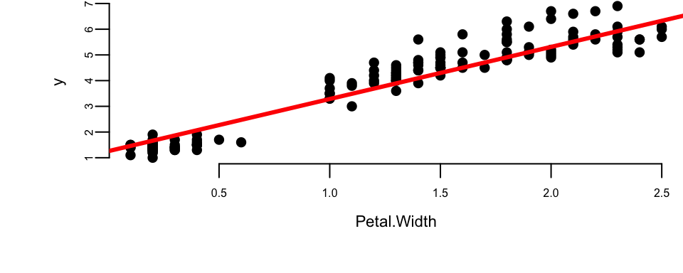
Let’s compare it to the standard estimation algorithm
m = lm(Petal.Length~Petal.Width, data=iris)| (Intercept) | Petal.Width |
|---|---|
| 1.1 | 2.2 |
The values found by gradient descent are very close to the ones found by the standard OLS algorithm.
The standard way to monitor the convergence of the gradient descent algorithm is to plot the value of the loss function at each iteration.
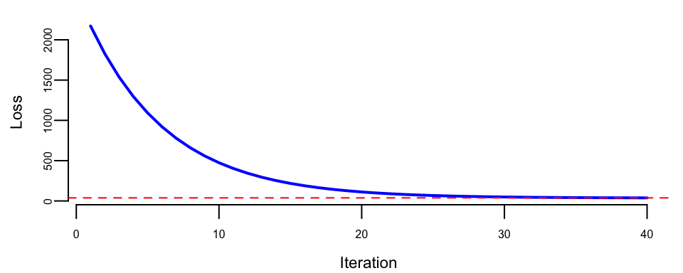
We can see that the loss smoothly decays to the minimum value. This is because our loss function is convex (quadratic function of the parameters \(\theta\)), meaning that it has a single global minimum and no local minima, and our learning rate of \(0.0001\) is small enough to ensure that the algorithm does not overshoot the minimum. However, this is often not the case for more complex models, such as deep neural networks. In those cases, the loss function may oscillate between multiple local minima and saddle points, which can make the convergence of the gradient descent algorithm difficult. In practice, we often use a larger learning rate and a modified version of the gradient descent algorithm, such as Nesterov accelerated gradient descent (NAG) or Adam, to help with the convergence.
Example 20.2 (Logistic Regression) Logistic regression is a generalized linear model (GLM) with a logit link function, defined as: \[ \log \left(\frac{p}{1-p}\right) = \theta_0 + \theta_1 x_1 + \ldots + \theta_p x_p, \] where \(p\) is the probability of the positive class. The negative log-likelihood function for logistic regression is a cross-entropy loss \[ l(\theta) = - \sum_{i=1}^n \left[ y_i \log p_i + (1-y_i) \log (1-p_i) \right], \] where \(p_i = 1/\left(1 + \exp(-\theta_0 - \theta_1 x_{i1} - \ldots - \theta_p x_{ip})\right)\). The derivative of the negative log-likelihood function is \[ \nabla l(\theta) = - \sum_{i=1}^n \left[ y_i - p_i \right] \begin{pmatrix} 1 \\ x_{i1} \\ \vdots \\ x_{ip} \end{pmatrix}. \] In matrix notation, we have \[ \nabla l(\theta) = - X^\top (y - p). \] Let’s implement the gradient descent algorithm now.
y = ifelse(iris$Species=="setosa",1,0)
x = cbind(rep(1,150),iris$Sepal.Length)
lrgd  = function(x,y, alpha, n_iter) {
  theta <- matrix(c(0, 0), nrow = 2, ncol = 1)
  for (i in 1:n_iter) {
    # compute gradient
    p = 1/(1+exp(-x %*% theta))
    grad <- -t(x) %*% (y - p)
    # update theta
    theta <- theta - alpha * grad
  }
  return(theta)
}
theta = lrgd(x,y,0.005,20000)
The gradient descent parameters are
| Intercept (\(\theta_0\)) | Sepal.Length (\(\theta_1\)) |
|---|---|
| 28 | -5.2 |
And the plot is
plot(x[,2],y,pch=16, xlab="Sepal.Length")
lines(x[,2],p,type='p', pch=16,col="red")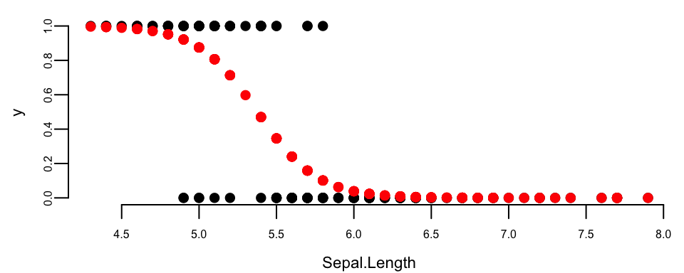
Let’s compare it to the standard estimation algorithm
| term | estimate | std.error | statistic | p.value |
|---|---|---|---|---|
| x1 | 27.8 | 4.83 | 5.8 | 0 |
| x2 | -5.2 | 0.89 | -5.8 | 0 |
20.2 Stochastic Gradient Descent
Stochastic gradient descent (SGD) is a variant of the gradient descent algorithm. The main difference is that instead of computing the gradient over the entire dataset, SGD computes the gradient over a randomly selected subset of the data. This allows SGD to be applied to estimate models when the dataset is too large to fit into memory, which is often the case with deep learning models. The SGD algorithm replaces the gradient of the negative log-likelihood function with the gradient computed over a randomly selected subset of the data: \[ \nabla l(\theta) \approx \dfrac{1}{|B|} \sum_{i \in B} \nabla l(y_i, f(x_i, \theta)), \] where \(B \subseteq \{1,2,\ldots,n\}\) is a batch (random subset) sampled from the dataset, and \(|B|\) denotes the batch size (number of samples in the batch). This method can be interpreted as gradient descent using noisy gradients, which are typically called mini-batch gradients.
SGD is based on the idea of stochastic approximation introduced by Robbins and Monro (1951). Stochastic approximation simply replaces the expected gradient with its Monte Carlo approximation.
In a small mini-batch regime, when \(|B| \ll n\) and typically \(|B| \in \{32,64,\ldots,1024\}\), it was shown that SGD converges faster than standard gradient descent, does converge to minimizers of strongly convex functions (the negative log-likelihood of an exponential-family model is convex, and strongly convex under \(L_2\) regularization) (Bottou, Curtis, and Nocedal 2018), and is more robust to noise in the data (Hardt, Recht, and Singer 2016). Further, SGD can avoid saddle points, which is often an issue with deep learning loss functions. In the case of multiple minima, SGD can find a good solution (Keskar et al. 2016; LeCun et al. 2002), meaning that out-of-sample performance is often worse when trained with large-batch methods compared to small-batch methods.
Now, we implement SGD for logistic regression and compare performance for different batch sizes
Now run our SGD algorithm with different batch sizes.
set.seed(92) # kuzy
ind = sample(150)
y = ifelse(iris$Species=="setosa",1,0)[ind] # shuffle data
x = cbind(rep(1,150),iris$Sepal.Length)[ind,] # shuffle data
nit=200000
lr = 0.01
th1 = lrgd_minibatch(x,y,lr,nit,5)
th2 = lrgd_minibatch(x,y,lr,nit,15)
th3 = lrgd_minibatch(x,y,lr,nit,30)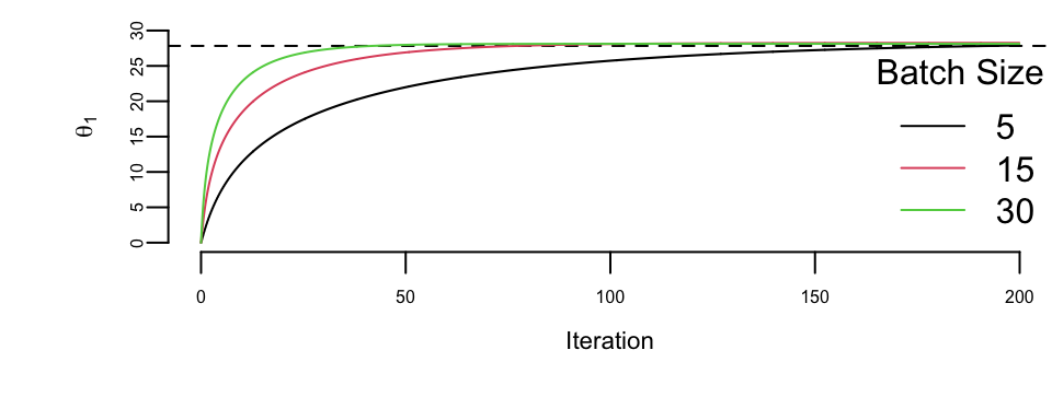
We run it with 200000 iterations and the learning rate of 0.01 and plot the values of \(\theta_1\) every 1000 iterations. There are a couple of important points we need to highlight when using SGD. First, we shuffle the data before using it. The reason is that if the data are sorted in any way (e.g., by date or by value of one of the inputs), then data within batches can be highly correlated, which reduces the convergence speed. Shuffling helps avoid this issue, but it also implicitly treats the dataset as exchangeable; for time series and streaming data, shuffling is typically inappropriate (see Chapter 15). Second, the larger the batch size, the smaller the number of iterations required for convergence, which is something we would expect. However, in this specific example, from the computational point of view, the batch size does not change the number of calculations required overall. Let’s look at the same plot, but scale the x-axis according to the amount of computations
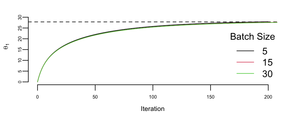
There are several important considerations about choosing the batch size for SGD.
- The larger the batch size, the more memory is required to store the data.
- Parallelization is more efficient with larger batch sizes. Modern hardware supports parallelization of matrix operations, which is the main operation in SGD. The larger the batch size, the more efficient the parallelization is. Usually there is a sweet spot \(|B|\) for the batch size, which is the largest batch size that can fit into memory or be parallelized. This means it takes the same amount of time to compute an SGD step for batch size \(1\) and \(B\).
- Third, the larger the batch size, the less noise in the gradient. This means that the larger the batch size, the more accurate the gradient is. However, it was empirically shown that in many applications we should prefer noisier gradients (small batches) to obtain high-quality solutions when the objective function (negative log-likelihood) is non-convex (Keskar et al. 2016).
20.3 Automatic Differentiation (Backpropagation)
Gradient descent requires computing gradients at each iteration. But how do we efficiently compute gradients for complex compositional functions like deep neural networks? The answer lies in automatic differentiation, a technique whose development is intertwined with the history of neural networks themselves.
Original neural networks (Perceptrons) proposed by Rosenblatt (1958) were single-layer feedforward networks with a threshold activation function in the output layer. They were trained using an error-correction (perceptron) learning rule.
The delta rule of Widrow and Hoff (1960) provides a simple gradient-based learning algorithm for single-layer networks with a differentiable activation. For a single-layer perceptron with output \(\hat{y} = \sigma(w^\top x + b)\), where \(\sigma\) is an activation function, the delta rule updates weights as: \[ w^{t+1} = w^t - \alpha (\hat{y} - y) \sigma'(w^\top x + b) x \] where \(\alpha\) is the learning rate, and \(y\) is the target output. This rule is intuitive: when the prediction \(\hat{y}\) differs from the target \(y\), we adjust the weights proportionally to the input \(x\) and the derivative of the activation function.
However, the delta rule encounters a fundamental limitation with multi-layer networks. Consider a network with hidden layers: \(h = \sigma_1(W_1 x + b_1)\) and \(\hat{y} = \sigma_2(W_2 h + b_2)\). To update weight \(W_1\) in the first layer, we need to compute \(\frac{\partial L}{\partial W_1}\), where \(L\) is the loss function. By the chain rule: \[ \frac{\partial L}{\partial W_1} = \frac{\partial L}{\partial \hat{y}} \cdot \frac{\partial \hat{y}}{\partial h} \cdot \frac{\partial h}{\partial W_1} \]
The delta rule could not efficiently compute this gradient through multiple layers, as it lacked a systematic method for propagating error signals backward through the network. This meant that while single-layer networks could be trained effectively, there was no practical way to train deeper architectures that could learn more complex representations.
The inability to train multi-layer networks led to the first AI winter in the late 1960s and 1970s. Minsky and Papert (1969) demonstrated that single-layer perceptrons could not solve non-linearly separable problems like XOR, and without a method to train deeper architectures, neural network research largely stagnated.
Unknown to most of the neural network community at the time, the solution to training multi-layer networks through systematic application of the chain rule was being developed independently by several researchers. In the Soviet Union, Galushkin (1973) developed methods for training multi-layer networks using gradient-based approaches, though this work remained largely unknown in the West due to the Cold War.
In the Western literature, the first clear formulation of backpropagation came from P. Werbos (1974), who in his 1974 PhD thesis at Harvard University introduced the idea of using the chain rule to efficiently compute gradients in multi-layer networks. Werbos explicitly showed how to propagate derivatives backward through a network by decomposing complex functions into simpler components. He refined these ideas further in P. J. Werbos (1982), demonstrating how reverse-mode automatic differentiation could be applied to train neural networks efficiently.
The same mathematical principle, systematic application of the chain rule for computing derivatives, was being applied in a different context around the same time. Nelder and Wedderburn (1972) introduced Generalized Linear Models (GLMs) and developed an iteratively reweighted least squares (IRLS) algorithm that explicitly used the chain rule to compute gradients for maximum likelihood estimation.
To understand their contribution, consider a GLM where the response variable \(y_i\) follows a distribution from the exponential family with mean \(\mu_i\). The model relates the mean to the predictors through a link function \(g(\cdot)\): \[ g(\mu_i) = \eta_i = x_i^\top \theta \] where \(x_i\) is the vector of predictors for observation \(i\), \(\theta\) is the parameter vector, and \(\eta_i\) is the linear predictor. For example, in logistic regression (which we saw in Example 20.2), we have \(g(\mu) = \log(\mu/(1-\mu))\) (the logit link).
The key innovation of Nelder and Wedderburn was recognizing that computing the gradient of the log-likelihood with respect to \(\theta\) requires systematic application of the chain rule. Specifically, for observation \(i\), the gradient decomposes as: \[ \frac{\partial \log L}{\partial \theta_j} = \frac{\partial \log L}{\partial \mu_i} \cdot \frac{\partial \mu_i}{\partial \eta_i} \cdot \frac{\partial \eta_i}{\partial \theta_j} \]
The first term, \(\partial \log L/\partial \mu_i\), depends on the specific distribution (e.g., Gaussian, Bernoulli, Poisson). For exponential family distributions, this takes the form \((y_i - \mu_i)/V(\mu_i)\), where \(V(\mu_i)\) is the variance function. The second term, \(\partial \mu_i/\partial \eta_i\), is the derivative of the inverse link function. The third term is simply \(x_{ij}\), the \(j\)-th predictor value.
Combining these using the chain rule, they derived the gradient: \[ \frac{\partial \log L}{\partial \theta_j} = \sum_{i=1}^n \frac{(y_i - \mu_i)}{V(\mu_i)} \cdot \frac{\partial \mu_i}{\partial \eta_i} \cdot x_{ij} \]
For the Newton-Raphson optimization method (also known as Fisher scoring when using expected second derivatives), they needed to compute the Hessian matrix. Applying the chain rule again to the gradient yields the Fisher information matrix with elements: \[ \mathcal{I}_{jk} = \sum_{i=1}^n w_i x_{ij} x_{ik} \] where the weight \(w_i = \left(\frac{\partial \mu_i}{\partial \eta_i}\right)^2 / V(\mu_i)\) is itself computed by the chain rule. This leads to the iteratively reweighted least squares algorithm, where at each iteration \(t\) we solve: \[ \theta^{t+1} = \theta^t + \mathcal{I}(\theta^t)^{-1} \nabla \log L(\theta^t) \]
The success of GLMs demonstrated that chain rule-based gradient computation was practically valuable for fitting sophisticated models. Nelder and Wedderburn published their GLM framework in 1972, just two years before Werbos’s PhD thesis on backpropagation; both independently discovered that systematic chain rule application could efficiently compute gradients in compositional models. Despite these parallel discoveries, backpropagation did not enter mainstream neural network research until Rumelhart, Hinton, and Williams (1986) popularized it under the name backpropagation.
To calculate the value of the gradient vector at each step of the optimization process, gradient descent algorithms require calculations of derivatives. In general, there are three different ways to calculate those derivatives. First, we can do it by hand. This is slow and error-prone. Second is numerical differentiation, when a gradient is approximated by a finite difference; for some small \(h\), calculate \(f'(x) \approx (f(x+h)-f(x))/h\), which requires two function evaluations. This approach is not backward stable (Griewank, Kulshreshtha, and Walther 2012), meaning that for a small perturbation in input value \(x\), the calculated derivative is not the correct one. Lastly, we can use symbolic differentiation or automatic differentiation (AD) which has been used for decades in computer algebra systems such as Mathematica or Maple. Symbolic differentiation uses a tree form representation of a function and applies the chain rule to the tree to calculate the symbolic derivative of a given function.
The advantage of symbolic calculations is that the analytical representation of the derivative is available for further analysis, for example, when derivative calculation is an intermediate step of the analysis. A third way to calculate a derivative is to use automatic differentiation (AD). Similar to symbolic differentiation, AD recursively applies the chain rule and calculates the exact value of the derivative, thus avoiding the problem of numerical instability. The difference between AD and symbolic differentiation is that AD provides the value of the derivative evaluated at a specific point, rather than an analytical representation of the derivative.
AD does not require analytical specification and can be applied to a function defined by a sequence of algebraic manipulations, logical and transcendent functions applied to input variables and specified in computer code. AD can differentiate complex functions which involve IF statements and loops, and AD can be implemented using either forward or backward mode. Consider an example of calculating a derivative of the logistic function \[ f(x) = \frac{1}{1+e^{-(Wx+b)}}. \]
Which is implemented as follows:
Given the function \(f(x) = \frac{1}{1+e^{-(Wx+b)}} = v_3\), the derivative with respect to \(w\) is given by the chain rule. Recall that for the sigmoid function \(\sigma(z) = 1/(1+e^{-z})\), we have \(\sigma'(z) = \sigma(z)(1-\sigma(z))\). Therefore: \[ \frac{\partial f}{\partial w} = \frac{\partial v_3}{\partial v_2} \cdot \frac{\partial v_2}{\partial v_1} \cdot \frac{\partial v_1}{\partial w} = v_3(1-v_3) \cdot 1 \cdot x \]
\[ \frac{\partial f}{\partial b} = \frac{\partial v_3}{\partial v_2} \cdot \frac{\partial v_2}{\partial b} = v_3(1-v_3) \cdot 1 \]
In the forward mode, an auxiliary variable, called a dual number, will be added to each line of the code to track the value of the derivative associated with this line. In our example, if we set x=2, w=3, b=5, we get the calculations given in the table below.
| Function calculations | Derivative calculations |
|---|---|
1. v1 = w*x = 6 |
1. dv1 = w = 3 (derivative of v1 with respect to x) |
2. v2 = v1 + b = 11 |
2. dv2 = dv1 = 3 (derivative of v2 with respect to x) |
3. v3 = 1/(1+exp(-v2)) = 0.99998 |
3. dv3 = dv2*v3*(1-v3) = 5e-05 |
Variables dv1,dv2,dv3 correspond to partial (local) derivatives of each intermediate variable v1,v2,v3 with respect to \(x\), and are called dual variables. Tracking for dual variables can either be implemented using source code modification tools that add new code for calculating the dual numbers or via operator overloading.
The reverse AD also applies the chain rule recursively but starts from the outer function, as shown in the table below.
| Function calculations | Derivative calculations |
|---|---|
1. v1 = w*x = 6 |
4. dv1 = dv2*dv2dv1 = 1.67e-05; df/dx = dv1*w = 5e-05 |
2. v2 = v1 + b = 11 |
3. dv2dv1 = 1; dv2 = dv3*dv3dv2 = 1.67e-05 |
3. v3 = 1/(1+exp(-v2)) = 0.99998 |
2. dv3 = dv4 = 1; dv3dv2 = v3*(1-v3) = 1.67e-05 |
4. v4 = v3 |
1. dv4 = 1 |
The key difference between forward and reverse mode is the direction of computation:
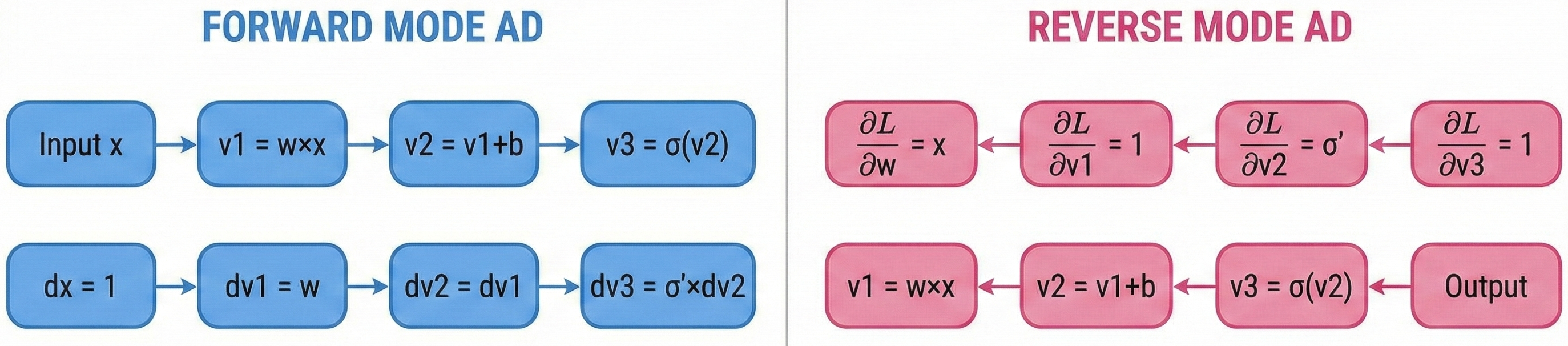
- Forward mode: Propagates derivatives with the computation, from inputs to outputs. Efficient when number of inputs < number of outputs.
- Reverse mode: Propagates derivatives against the computation, from outputs to inputs. Efficient when number of outputs < number of inputs.
For neural networks with millions of parameters (inputs to the loss function) but a single scalar loss (one output), reverse mode is dramatically more efficient, which is why backpropagation uses reverse mode AD.
Figure 20.3 shows a tree representation of the composition of affine and sigmoid functions (the first layer of our neural network). The numbers in the nodes are the values of the variables at a specific point, and the arrows show the flow of data. During the forward pass (solid arrows), the data flow from inputs (x, w, b) to the final output v3, and all intermediate variables are computed. During the backward pass (dashed arrows), the gradient values flow from the output back to the inputs by applying the chain rule to each variable.
graph LR
    %% Input nodes
    X["x = 2<br/>∇x = w × v3(1-v3)"]
    W["w = 3<br/>∇w = x × v3(1-v3)"]
    B["b = 5<br/>∇b = v3(1-v3)"]

    %% Computation nodes
    V1["v1 = w × x = 6<br/>∇v1 = v3(1-v3)"]
    V2["v2 = v1 + b = 11<br/>∇v2 = v3(1-v3)"]
    NEG["-v2 = -11"]
    EXP["exp(-v2) = 0.0000<br/>∇exp = -v3(1-v3)"]
    ONE["1"]
    ADD1["1 + exp(-v2) = 1.0000<br/>∇add = v3(1-v3)"]
    V3["v3 = 1/(1+exp(-v2)) = 0.99998<br/>∇v3 = 1"]

    %% Forward pass connections (solid arrows)
    X --> V1
    W --> V1
    V1 --> V2
    B --> V2
    V2 --> NEG
    NEG --> EXP
    ONE --> ADD1
    EXP --> ADD1
    ADD1 --> V3

    %% Backward pass connections (dashed arrows - gradient flow)
    V3 -.-> ADD1
    ADD1 -.-> EXP
    ADD1 -.-> ONE
    EXP -.-> NEG
    NEG -.-> V2
    V2 -.-> V1
    V2 -.-> B
    V1 -.-> W
    V1 -.-> X

    %% Styling
    classDef input fill:#e1f5fe,stroke:#0277bd,stroke-width:2px
    classDef computation fill:#f3e5f5,stroke:#7b1fa2,stroke-width:2px
    classDef constant fill:#e8f5e8,stroke:#388e3c,stroke-width:2px
    classDef output fill:#fff3e0,stroke:#f57c00,stroke-width:2px

    class X,W,B input
    class V1,V2,NEG,EXP,ADD1 computation
    class ONE constant
    class V3 output
For DL, derivatives are calculated by applying the reverse AD algorithm to a model which is defined as a superposition of functions. A model is defined either using a general-purpose language as it is done in PyTorch or through a sequence of function calls defined by framework libraries (e.g., in TensorFlow). Forward AD algorithms calculate the derivative with respect to a single input variable, but reverse AD produces derivatives with respect to all intermediate variables. For models with many parameters, it is much more computationally feasible to perform the reverse AD.
In the context of neural networks, the reverse AD algorithm is called backpropagation and was popularized in AI by Rumelhart, Hinton, and Williams (1986). According to Schmidhuber (2015), the first version of what we call today backpropagation was published in 1970 in a master’s thesis Linnainmaa (1970) and was closely related to the work of Ostrovskii, Volin, and Borisov (1971). However, similar techniques rooted in Pontryagin’s maximum principle were discussed in the context of multi-stage control problems (Arthur E. Bryson 1961; Arthur E. Bryson and Ho 1969). Dreyfus (1962) applies backpropagation to calculate the first-order derivative of a return function to numerically solve a variational problem. Later Dreyfus (1973) used backpropagation to derive an efficient algorithm to solve a minimization problem. The first neural network-specific version of backpropagation was proposed in P. Werbos (1974), and an efficient backpropagation algorithm was discussed in P. J. Werbos (1982).
Modern deep learning frameworks fully automate the process of finding derivatives using AD algorithms. For example, PyTorch relies on the autograd library which automatically finds gradients using the backpropagation algorithm. Here is a small code example using the autograd library in jax.
The code below implements a simple neural network with one hidden layer and uses backpropagation to find the gradient of the negative log-likelihood function. The model is trained on a synthetic dataset generated from a circle. The code uses the jax library, which is a high-performance numerical computing library that supports automatic differentiation.
## 1.0Note that inside the gradient descent function gd_step we use the grad function to calculate the gradient of the negative log-likelihood function with respect to the weights and biases. The jit decorator is used to compile the function for faster execution. The gd_step function updates the weights and biases using the calculated gradients and a learning rate of 0.02.
Finally, we can plot the decision boundary of the trained model
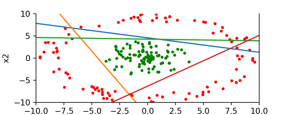
We can see that the model has learned to separate the two classes. Two of the lines are almost parallel, which is expected. We could have gotten away with using only three hidden units instead of four.
20.4 Advanced Optimization Methods
While the basic SGD algorithm introduced earlier works well for many problems, practitioners have developed numerous enhancements to improve convergence speed and stability. This section surveys the most important variants used in modern deep learning.
Momentum Methods
One limitation of vanilla SGD is that the descent in the loss function is not guaranteed at every iteration, and progress can be slow when gradients are noisy. To address this, momentum-based methods add memory to the search process by combining new gradient information with previous search directions (Polyak 1964). Empirically, momentum-based methods have been shown to have better convergence for deep learning networks (Sutskever et al. 2013). The gradient only influences changes in the velocity of the update, which then updates the variable:
\[ v^{k+1} = \mu v^k - t_k g((W,b)^k) \] \[ (W,b)^{k+1} = (W,b)^k + v^{k+1} \]
The hyperparameter \(\mu\) controls the damping effect on the rate of update of the variables. The physical analogy is the reduction in kinetic energy that allows to “slow down” the movements at the minima. This parameter can also be chosen empirically using cross-validation.
Nesterov’s momentum method (Nesterov 1983) (a.k.a. Nesterov acceleration) calculates the gradient at the point predicted by the momentum. One can view this as a look-ahead strategy with the updating scheme
\[ v^{k+1} = \mu v^k - t_k g((W,b)^k + \mu v^k) \] \[ (W,b)^{k+1} = (W,b)^k + v^{k+1} \]
Adaptive Learning Rate Methods
Another popular modification is AdaGrad (Duchi, Hazan, and Singer 2011), which adaptively scales the learning rate for each parameter based on the history of gradients:
\[ c^{k+1} = c^k + g(\theta^k)^2 \] \[ \theta^{k+1} = \theta^k - \frac{t_k}{\sqrt{c^{k+1}} + \epsilon} g(\theta^k) \]
where \(\epsilon\) is a small constant (e.g., \(\epsilon = 10^{-8}\)) to prevent division by zero. RMSprop (Hinton, Srivastava, and Swersky 2012) extends AdaGrad by using an exponentially weighted moving average of squared gradients:
\[ c^{k+1} = \rho c^k + (1-\rho) g(\theta^k)^2 \] \[ \theta^{k+1} = \theta^k - \frac{t_k}{\sqrt{c^{k+1}} + \epsilon} g(\theta^k) \]
The Adam method (Kingma and Ba 2014) combines RMSprop with momentum by maintaining exponentially weighted averages of both the gradient (first moment) and the squared gradient (second moment):
\[ m^{k+1} = \beta_1 m^k + (1-\beta_1) g(\theta^k) \] \[ c^{k+1} = \beta_2 c^k + (1-\beta_2) g(\theta^k)^2 \] \[ \theta^{k+1} = \theta^k - \frac{t_k}{\sqrt{\hat{c}^{k+1}} + \epsilon} \hat{m}^{k+1} \]
where \(\hat{m}^{k+1}\) and \(\hat{c}^{k+1}\) are bias-corrected estimates. The typical hyperparameter values are \(\beta_1 = 0.9\), \(\beta_2 = 0.999\), and \(\epsilon = 10^{-8}\).
The following table summarizes the key optimization methods:
| Method | Key Idea | Update Rule |
|---|---|---|
| SGD | Noisy gradient estimates | \(\theta^{k+1} = \theta^k - t_k g^k\) |
| Momentum | Accumulate gradient direction | \(v^{k+1} = \mu v^k - t_k g^k\); \(\theta^{k+1} = \theta^k + v^{k+1}\) |
| Nesterov | Look-ahead gradient | \(v^{k+1} = \mu v^k - t_k g(\theta^k + \mu v^k)\); \(\theta^{k+1} = \theta^k + v^{k+1}\) |
| AdaGrad | Per-parameter learning rates | Scale by \(1/\sqrt{\sum g^2}\) |
| RMSprop | Exponential moving average | Scale by \(1/\sqrt{\text{EMA}(g^2)}\) |
| Adam | Momentum + adaptive rates | Combines first and second moment estimates |
Second-Order Methods
Second-order methods solve the optimization problem by solving a system of nonlinear equations \(\nabla f(\theta) = 0\) using Newton’s method:
\[ \theta^{+} = \theta - \{ \nabla^2 f(\theta) \}^{-1} \nabla f(\theta) \]
We can see that SGD effectively approximates the inverse Hessian \(\{\nabla^2 f(\theta)\}^{-1}\) by \(t_k I\), where \(I\) is the identity matrix. The advantages of second-order methods include much faster convergence rates and insensitivity to the conditioning of the problem. However, in practice, second-order methods are rarely used for deep learning applications (Dean et al. 2012). The major disadvantage is the inability to train models using mini-batches as SGD does. Since typical deep learning models rely on large-scale datasets, computing and storing the Hessian becomes memory and computationally prohibitive.
20.5 Why Robbins-Monro?
The Robbins-Monro algorithm was introduced in their seminal 1951 paper “A Stochastic Approximation Method” Robbins and Monro (1951). The paper addressed the problem of finding the root of a function when only noisy observations are available.
Consider a function \(M(\theta)\) where we want to find \(\theta^*\) such that \(M(\theta^*) = \alpha\) for some target value \(\alpha\). In the original formulation, \(M(\theta)\) represents the expected value of some random variable \(Y(\theta)\):
\[M(\theta) = \E{Y(\theta)} = \alpha\]
The key insight is that we can only observe noisy realizations \(y(\theta)\) where:
\[y(\theta) = M(\theta) + \epsilon(\theta)\]
where \(\epsilon(\theta)\) is a zero-mean random error term.
The Robbins-Monro algorithm iteratively updates the estimate \(\theta_n\) using:
\[\theta_{n+1} = \theta_n - a_n(y(\theta_n) - \alpha)\]
where \(a_n\) is a sequence of positive step sizes that must satisfy:
\[\sum_{n=1}^{\infty} a_n = \infty \quad \text{and} \quad \sum_{n=1}^{\infty} a_n^2 < \infty\]
These conditions ensure that the algorithm can explore the entire space (first condition) while eventually converging (second condition).
Under appropriate conditions on \(M(\theta)\) (monotonicity and boundedness), the algorithm converges almost surely to \(\theta^*\):
\[\lim_{n \to \infty} \theta_n = \theta^* \quad \text{almost surely}\]
The convergence rate depends on the choice of step sizes. For \(a_n = c/n\) with \(c > 0\) and \(c\) sufficiently large, the mean squared error \(\E{(\theta_n - \theta^*)^2}\) decreases as \(O(1/n)\) (Robbins and Monro 1951).
This foundational work established the theoretical basis for stochastic approximation methods that are now widely used in machine learning, particularly in stochastic gradient descent and related optimization algorithms.
Connection to M-Estimation
The Robbins-Monro framework connects naturally to statistical estimation. Many estimands, including means, medians, quantiles, and regression coefficients, can be expressed as solutions to convex optimization problems:
\[\theta^* = \arg\min_{\theta \in \mathbb{R}^p} \E{\ell_\theta(X_i, Y_i)},\]
where \(\ell_\theta\) is a convex loss function. Under mild conditions, the optimum \(\theta^*\) satisfies the first-order condition: \[ \E{g_\theta(X_i, Y_i)} = 0, \tag{20.1}\]
where \(g_\theta\) is a subgradient of the loss. SGD can be viewed as applying the Robbins-Monro algorithm to find roots of this gradient condition using noisy samples.
20.6 The EM, ECM, and ECME Algorithms
Gradient descent is not the only iterative optimization algorithm used in statistics. When dealing with latent variables or missing data, directly computing gradients of the log-likelihood can be intractable. The Expectation-Maximization (EM) algorithm provides an elegant alternative that iteratively maximizes a surrogate function, avoiding explicit gradient computation while guaranteeing monotonic improvement in the likelihood.
First, define a function \(Q(\theta,\phi)\) such that \(Q(\theta) = Q(\theta,\theta)\) and it satisfies the domination condition \(Q(\theta,\phi) \leq Q(\theta,\theta)\) for all \(\phi\), i.e., \(Q\) minorizes the objective. Then define
\[\theta^{(g+1)} = \arg\max_{\theta \in \Theta} Q(\theta,\theta^{(g)})\]
Since \(Q(\theta,\phi) \leq Q(\theta,\theta)\) for any \(\phi\), maximizing \(Q(\theta,\theta^{(g)})\) over \(\theta\) guarantees monotone improvement. In order to prove convergence, you get a sequence of inequalities
\[Q(\theta^{(0)},\theta^{(0)}) \leq Q(\theta^{(1)},\theta^{(0)}) \leq Q(\theta^{(1)},\theta^{(1)}) \leq \ldots \leq Q\]
In many models we have to deal with a latent variable and require estimation where integration is also involved. For example, suppose that we have a triple \((y,z,\theta)\) with joint probability specification \(p(y,z,\theta) = p(y\mid z,\theta)p(z,\theta)\). This can occur in missing data problems and estimation problems in mixture models.
A standard application of the EM algorithm is to find
\[\arg\max_{\theta \in \Theta} \int_z p(y\mid z,\theta)p(z\mid\theta)dz\]
As we are just finding an optimum, you do not need the prior specification \(p(\theta)\). The EM algorithm finds a sequence of parameter values \(\theta^{(g)}\) by alternating between an expectation and a maximisation step. This still requires the numerical (or analytical) computation of the criteria function \(Q(\theta,\theta^{(g)})\) described below.
EM algorithms have been used extensively in mixture models and missing data problems. The EM algorithm uses the particular choice where
\[Q(\theta) = \log p(y\mid\theta) = \log \int p(y,z\mid\theta)dz\]
Here the likelihood has a mixture representation where \(z\) is the latent variable (missing data, state variable, etc.). This is termed a Q-maximization algorithm with:
\[Q(\theta,\theta^{(g)}) = \int \log p(y,z\mid\theta)p(z\mid\theta^{(g)},y)dz = \E[z\mid\theta^{(g)},y]{\log p(y,z\mid\theta)}\]
To implement EM you need to be able to calculate \(Q(\theta,\theta^{(g)})\) and optimize at each iteration.
The EM algorithm and its extensions ECM and ECME are methods of computing maximum likelihood estimates or posterior modes in the presence of missing data. Let the objective function be \(\ell(\theta) = \log p(\theta\mid y) + c(y)\), where \(c(y)\) is a possibly unknown normalizing constant that does not depend on \(\theta\), and \(y\) denotes observed data. We have a mixture representation,
\[p(\theta\mid y) = \int p(\theta,z\mid y)dz = \int p(\theta\mid z,y)p(z\mid y)dz\]
where distribution of the latent variables is \(p(z\mid\theta,y) = p(y\mid\theta,z)p(z\mid\theta)/p(y\mid\theta)\).
In some cases, the complete data log-posterior is simple enough for \(\arg\max_{\theta} \log p(\theta\mid z,y)\) to be computed in closed form. The EM algorithm alternates between the Expectation and Maximization steps for which it is named. The E-step and M-step computes
\[Q(\theta\mid\theta^{(g)}) = \E[z\mid\theta^{(g)},y]{\log p(y,z\mid\theta)} = \int \log p(y,z\mid\theta)p(z\mid\theta^{(g)},y)dz\]
\[\theta^{(g+1)} = \arg\max_{\theta} Q(\theta\mid\theta^{(g)})\]
This has an important monotonicity property that ensures \(\ell(\theta^{(g)}) \leq \ell(\theta^{(g+1)})\) for all \(g\). In fact, the monotonicity proof given by Dempster et al. (1977) shows that any \(\theta\) with \(Q(\theta,\theta^{(g)}) \geq Q(\theta^{(g)},\theta^{(g)})\) also satisfies the log-likelihood inequality \(\ell(\theta) \geq \ell(\theta^{(g)})\).
In problems with many parameters, the M-step of EM may be difficult. In this case \(\theta\) may be partitioned into components \((\theta_1,\ldots,\theta_k)\) in such a way that maximizing \(\log p(\theta_j\mid\theta_{-j},z,y)\) is easy. The ECM algorithm pairs the EM algorithm’s E-step with \(k\) conditional maximization (CM) steps, each maximizing \(Q\) over one component \(\theta_j\) with each component of \(\theta_{-j}\) fixed at the most recent value. Due to the fact that each CM step increases \(Q\), the ECM algorithm retains the monotonicity property. The ECME algorithm replaces some of ECM’s CM steps with maximizations over \(\ell\) instead of \(Q\). Liu and Rubin (1994) show that doing so can greatly increase the rate of convergence.
Seen through the optimization lens, ECM is a form of block coordinate ascent on a surrogate objective: it improves parameters one block at a time while holding the rest fixed. This contrasts with SGD, which takes small stochastic steps along noisy gradients of a single objective; both are iterative methods, but they trade off different sources of computational convenience (closed-form block updates versus cheap gradient estimates).
In many cases we will have a parameter vector \(\theta = (\beta,\nu)\) partitioned into its components and a missing data vector \(z = (\lambda,\omega)\). Then we compute the \(Q(\beta,\nu\mid\beta^{(g)},\nu^{(g)})\) objective function and then compute E- and M steps from this to provide an iterative algorithm for updating parameters. To update the hyperparameter \(\nu\) we can maximize the fully data posterior \(p(\beta,\nu\mid y)\) with \(\beta\) fixed at \(\beta^{(g+1)}\). The algorithm can be summarized as follows:
\[\beta^{(g+1)} = \arg\max_{\beta} Q(\beta\mid\beta^{(g)},\nu^{(g)}) \quad \text{where} \quad Q(\beta\mid\beta^{(g)},\nu^{(g)}) = \E[z\mid\beta^{(g)},\nu^{(g)},y]{\log p(y,z\mid\beta,\nu^{(g)})}\]
\[\nu^{(g+1)} = \arg\max_{\nu} \log p(\beta^{(g+1)},\nu\mid y)\]
Example 20.3 Simulated Annealing (SA) is a simulation-based approach to finding
\[\hat{\theta} = \arg\max_{\theta \in \Theta} H(\theta)\]
\[\pi_J(\theta) = \frac{e^{JH(\theta)}}{\int e^{JH(\theta)}d\mu(\theta)}\]
where \(J\) is a temperature parameter. Instead of looking at derivatives and performing gradient-based optimization, you can simulate from the sequence of densities. This forms a time-homogeneous Markov chain, and under suitable regularity conditions on the relaxation schedule for the temperature we have \(\theta^{(g)} \to \hat{\theta}\). The main caveat is that we need to know the criterion function \(H(\theta)\) to evaluate the Metropolis probability for sampling from the sequence of densities. This is not always available.
An interesting generalisation which is appropriate in latent variable mixture models is the following. Suppose that \(H(\theta) = \E[z\mid\theta]{H(z,\theta)}\) is unavailable in closed-form where, without loss of generality we assume that \(H(z,\theta) \geq 0\). In this case, we can use latent variable simulated annealing (LVSA) methods. Define a joint probability distribution for \(z_J = (z_1,\ldots,z_J)\) as
\[\pi_J(z_J,\theta) \propto \prod_{j=1}^J H(z_j,\theta)p(z_j\mid\theta)\mu(\theta)\]
for some measure \(\mu\) which ensures integrability of the joint. This distribution has the property that its marginal distribution on \(\theta\) is given by
\[\pi_J(\theta) \propto \E[z\mid\theta]{H(z,\theta)}^J \mu(\theta) = e^{J \ln H(\theta)}\mu(\theta)\]
By the simulated annealing argument we see that this marginal collapses on the maximum of \(\ln H(\theta)\). The advantage of this approach is that it is typically straightforward to sample with MCMC from the conditionals:
\[\pi_J(z_i\mid\theta) \sim H(z_j,\theta)p(z_j\mid\theta) \quad \text{and} \quad \pi_J(\theta\mid z) \sim \prod_{j=1}^J H(z_j,\theta)p(z_j\mid\theta)\mu(\theta)\]
Jacquier, Johannes, and Polson (2007) apply this framework to finding MLE estimates for commonly encountered latent variable models. The LVSA approach is particularly useful when the criterion function involves complex integrals that make direct optimization challenging, but where sampling from the conditional distributions remains tractable.
20.7 Conclusion
This chapter has covered the computational foundations of training deep learning models. Several key insights emerge:
Gradient Descent as the Foundation: While classical statistical methods rely on second-order optimization (Newton-Raphson, BFGS), deep learning’s scale demands first-order methods. Gradient descent, despite its simplicity, remains effective because it requires only gradient information, which scales linearly with the number of parameters.
Stochastic Approximation: The Robbins-Monro framework provides theoretical justification for SGD: noisy gradient estimates, when properly scheduled, converge to the true optimum. Mini-batch SGD exploits this insight, trading exact gradients for computational efficiency and, counterintuitively, often better generalization through implicit regularization.
Automatic Differentiation: The backpropagation algorithm is simply reverse-mode automatic differentiation applied to neural networks. Understanding this connection reveals why modern frameworks (PyTorch, JAX) can automatically compute gradients for arbitrary computational graphs. The key insight is that reverse mode is efficient when outputs are few and parameters are many, precisely the situation in supervised learning.
Advanced Optimizers: Building on vanilla SGD, momentum methods accelerate convergence by accumulating gradient information, while adaptive methods (AdaGrad, RMSprop, Adam) automatically tune per-parameter learning rates. These innovations have proven essential for training deep networks efficiently, though the optimal choice remains problem-dependent.
Beyond Gradients: The EM algorithm provides an alternative optimization paradigm for latent variable models, avoiding explicit gradient computation through clever algebraic manipulation. Simulated annealing offers yet another approach, using stochastic sampling to escape local minima.
The practical success of SGD and its variants remains somewhat surprising from a theoretical perspective. Why does an algorithm designed for convex optimization work so well on highly non-convex loss landscapes? Ongoing research suggests that the geometry of over-parameterized networks may be more benign than previously thought: saddle points abound, but local minima tend to generalize well. Understanding these phenomena remains an active area of research at the intersection of optimization theory and deep learning.
Exercises
Pen-and-Pencil
Exercise 20.1 (Gradient Descent) Consider minimizing \(f(x) = x^2 + 4x + 5\).
- Find the derivative \(f'(x)\).
- Starting from \(x_0 = 5\), perform 3 iterations of gradient descent with learning rate \(\eta = 0.3\).
- What is the optimal \(x^*\)? Compare with your result after 3 iterations.
- Plot the convergence of \(x\) and \(f(x)\) over 20 iterations.
Exercise 20.2 (Backpropagation) For the 2-2-1 network from the Neural Network Forward Pass exercise (Ch18), compute the gradients:
Given: \(x = (1, 2)^T\), true label \(y = 1\), learning rate \(\eta = 0.1\)
Recall the forward-pass results:
- \(z^{(1)} = (0, 0.9)^T\), \(a^{(1)} = (0, 0.9)^T\)
- \(z^{(2)} = 1.22\), \(\hat{y} = 0.772\)
- Calculate \(\frac{\partial L}{\partial z^{(2)}}\) where \(L\) is binary cross-entropy.
- Calculate \(\frac{\partial L}{\partial W_2}\) and \(\frac{\partial L}{\partial b_2}\).
- Calculate \(\frac{\partial L}{\partial a^{(1)}}\) (backpropagate through \(W_2\)).
- Update \(W_2\) using gradient descent with learning rate 0.1.
Exercise 20.3 (Newton’s Method versus Gradient Descent) Consider the quadratic objective \[ f(x) = \frac{1}{2} x^\top A x - b^\top x, \qquad x \in \mathbb{R}^d, \] where \(A\) is a symmetric positive definite \(d \times d\) matrix and \(b \in \mathbb{R}^d\). This chapter’s Second-Order Methods section poses the motivating question directly: Newton’s method uses curvature information to take more efficient steps than gradient descent, so why does deep learning rely on first-order methods instead?
- Derive the gradient \(\nabla f(x)\) and the Hessian \(\nabla^2 f(x)\).
- Write the gradient descent update with fixed step size \(\alpha\), and the Newton update \(x^{t+1} = x^t - \{\nabla^2 f(x^t)\}^{-1} \nabla f(x^t)\), both specialized to this \(f\).
- Show algebraically that, starting from any \(x^0\), Newton’s method reaches the minimizer \(x^* = A^{-1}b\) in exactly one step. Explain why this does not happen for gradient descent, and why the one-step argument does not carry over to a non-quadratic objective.
- For gradient descent with fixed step size \(\alpha\), state a condition on \(\alpha\) relative to the eigenvalues of \(A\) that guarantees convergence.
- Newton’s method looks strictly better after part (c). Explain why it is nonetheless impractical for deep learning models with \(d\) in the millions or billions: compare the storage cost of the Hessian (\(O(d^2)\) entries) to that of the gradient (\(O(d)\) entries), and the cost of solving the Newton system (equivalently, factoring the Hessian, \(O(d^3)\) by standard methods such as Cholesky or LU decomposition) to the cost of one gradient step (\(O(d)\) via a single backpropagation pass, as in the Automatic Differentiation section of this chapter).
- Illustrate parts (c)-(e) numerically in R for a small example.
Exercise 20.4 (Robbins-Monro Step-Size Conditions) The Why Robbins-Monro? section states that the recursion \(\theta_{n+1} = \theta_n - a_n\,(y(\theta_n) - \alpha)\) converges almost surely to the root \(\theta^*\) provided the positive step sizes satisfy the two summability conditions \[ \sum_{n=1}^{\infty} a_n = \infty \qquad\text{and}\qquad \sum_{n=1}^{\infty} a_n^2 < \infty . \] The first condition guarantees the iterates can travel far enough to reach \(\theta^*\) from any starting point; the second forces the steps to shrink fast enough that the observation noise averages out. This exercise pins down which schedules satisfy them and shows what breaks when they do not.
For the power-law family \(a_n = c/n^p\) with \(c > 0\) and \(p > 0\), use the \(p\)-series test to find the exact range of \(p\) for which both conditions hold. Does the constant \(c\) affect the answer?
Classify the schedules \(a_n = c\) (constant, \(p = 0\)), \(a_n = c/\sqrt{n}\) (\(p = 1/2\)), \(a_n = c/n^{0.9}\) (\(p = 0.9\)), \(a_n = c/n\) (\(p = 1\)), and \(a_n = c/n^2\) (\(p = 2\)) against your answer to (a). For each schedule that fails a condition, state which one fails and give a one-sentence description of what goes wrong in the algorithm.
In Python, verify the classification numerically by computing the partial sums \(\sum_{n=1}^{N} a_n\) and \(\sum_{n=1}^{N} a_n^2\) (with \(c = 1\)) up to \(N = 10^6\) for the five schedules. Confirm that the divergent sums keep growing with \(N\) while the convergent ones have essentially reached their limits.
Simulate the scalar recursion with \(M(\theta) = \theta\), target \(\alpha = 5\), i.i.d. noise \(\epsilon_n \sim N(0, \sigma^2 = 4)\), and \(\theta_0 = 0\), that is \(\theta_{n+1} = \theta_n - a_n(\theta_n + \epsilon_n - \alpha)\), over \(5000\) replications and \(500\) steps. For \(a_n = 1/n\) (both conditions hold) plot \(n\cdot\widehat{\E{(\theta_n - \alpha)^2}}\) against \(n\) and confirm it is flat near \(\sigma^2\), the \(O(1/n)\) rate quoted in the chapter. For the constant step \(a_n = 0.1\) plot \(\widehat{\E{(\theta_n - \alpha)^2}}\) (without the factor \(n\)) and show it plateaus at a strictly positive value. Connect each behaviour to the condition it satisfies or fails.
The stall predicted for a too-fast schedule (\(p > 1\)) needs a problem whose gradient stays bounded. On \(f(\theta) = |\theta - 5|\), whose subgradient \(\operatorname{sign}(\theta - 5)\) has magnitude \(1\), the total distance travelled from \(\theta_0\) is at most \(\sum_n a_n\). Run subgradient descent from \(\theta_0 = 0\) with the summable schedule \(a_n = 1/n^2\) and with the divergent schedule \(a_n = 1/n\), and show numerically that the first stalls short of the target while the second reaches it. Relate this to the first Robbins-Monro condition.
Exercise 20.5 (True/False: Optimization)
A learning rate that’s too small always leads to slower convergence but never affects the final solution quality.
Mini-batch SGD with batch size \(n\) (full dataset) is equivalent to gradient descent.
The Adam optimizer adapts the learning rate differently for each parameter.
Momentum always helps optimization and never hurts.
Neural network loss functions are typically convex.
Computing
Exercise 20.6 (Learning Rate Selection) For the function \(f(x) = x^4 - 3x^2 + 2\):
- Plot the function for \(x \in [-2, 2]\).
- Starting from \(x_0 = 1.5\), compare convergence with learning rates \(\eta = 0.01, 0.1, 0.5\).
- What happens with \(\eta = 1\)? Explain.
- Implement a simple line search to adaptively choose the learning rate.
Exercise 20.7 (Stochastic Gradient Descent) You have data \((x_i, y_i)\) for \(i = 1, ..., 1000\) and want to minimize: \[ L(\theta) = \frac{1}{n}\sum_{i=1}^n (y_i - \theta x_i)^2 \]
- Write the full gradient \(\nabla L(\theta)\) and the stochastic gradient for a single sample.
- Compare 1 epoch of full GD vs SGD with batch size 1 in terms of gradient computations.
- Implement mini-batch SGD with batch size 32 and compare to full-batch GD.
- Why might SGD converge to a better solution than full-batch GD in neural networks?
Exercise 20.8 (Momentum) Compare vanilla SGD with momentum-based SGD.
The momentum update is: \[ v_t = \beta v_{t-1} + \nabla L(\theta_t) \] \[ \theta_{t+1} = \theta_t - \eta v_t \]
- Explain intuitively why momentum helps optimization.
- For \(f(x, y) = x^2 + 100y^2\), an ill-conditioned quadratic (condition number 100), starting at \((5, 5)\), compare 100 iterations of SGD vs momentum (\(\beta = 0.9\)).
- What happens if \(\beta\) is too large (e.g., 0.99)?
- Describe Nesterov momentum and its advantage.
Exercise 20.9 (Adam Optimizer) The Adam optimizer combines momentum with adaptive learning rates.
Given: \(\beta_1 = 0.9\), \(\beta_2 = 0.999\), \(\epsilon = 10^{-8}\), \(\eta = 0.001\)
Updates: \[ m_t = \beta_1 m_{t-1} + (1 - \beta_1) g_t \] \[ c_t = \beta_2 c_{t-1} + (1 - \beta_2) g_t^2 \] \[ \hat{m}_t = m_t / (1 - \beta_1^t), \quad \hat{c}_t = c_t / (1 - \beta_2^t) \] \[ \theta_{t+1} = \theta_t - \eta \hat{m}_t / (\sqrt{\hat{c}_t} + \epsilon) \]
- Explain what \(m_t\) and \(c_t\) track.
- Why is bias correction (\(\hat{m}_t\), \(\hat{c}_t\)) necessary?
- Implement Adam for \(f(x) = x^4 - 3x^2 + 2\) and compare to vanilla SGD.
- When might you prefer SGD with momentum over Adam?
Exercise 20.10 (EM Algorithm for a Two-Component Gaussian Mixture) Consider data with a latent component indicator \(z_i \in \{1,2\}\) and \[ P(z_i = 1) = \pi, \qquad y_i \mid z_i = k \overset{\text{i.i.d.}}{\sim} N(\mu_k, \sigma_k^2), \quad k = 1,2. \] The marginal density of \(y_i\) is \(\pi N(y_i;\mu_1,\sigma_1^2) + (1-\pi) N(y_i;\mu_2,\sigma_2^2)\), so the observed-data log-likelihood is \[ \ell(\theta) = \sum_{i=1}^n \log\Big[\pi N(y_i;\mu_1,\sigma_1^2) + (1-\pi) N(y_i;\mu_2,\sigma_2^2)\Big], \qquad \theta = (\pi,\mu_1,\mu_2,\sigma_1^2,\sigma_2^2). \] The log of a sum makes \(\ell(\theta)\) awkward to maximize directly. The EM algorithm from this chapter avoids this by working with the complete-data likelihood and the \(Q\)-function instead.
- Simulate \(n=500\) observations in R with true parameters \(\pi = 0.4\), \(\mu_1 = -2\), \(\mu_2 = 3\), \(\sigma_1 = 1\), \(\sigma_2 = 1.5\). Set a seed. Plot a histogram of the simulated data.
- Using the \(Q\)-function from this chapter, \(Q(\theta,\theta^{(g)}) = \E[z\mid\theta^{(g)},y]{\log p(y,z\mid\theta)}\), show that the E-step reduces to computing the responsibility \[ \gamma_i^{(g)} = P(z_i = 1 \mid y_i,\theta^{(g)}) = \frac{\pi^{(g)} N(y_i;\mu_1^{(g)},\sigma_1^{2(g)})}{\pi^{(g)} N(y_i;\mu_1^{(g)},\sigma_1^{2(g)}) + (1-\pi^{(g)}) N(y_i;\mu_2^{(g)},\sigma_2^{2(g)})}. \]
- Show that maximizing \(Q(\theta,\theta^{(g)}) = \sum_{i=1}^n \big[\gamma_i^{(g)}(\log\pi + \log N(y_i;\mu_1,\sigma_1^2)) + (1-\gamma_i^{(g)})(\log(1-\pi) + \log N(y_i;\mu_2,\sigma_2^2))\big]\) over \(\theta\) gives the M-step as responsibility-weighted means, variances, and mixing proportion.
- Implement the E-step and M-step in R, iterate until convergence, and track the observed-data log-likelihood \(\ell(\theta^{(g)})\) at every iteration.
- Plot \(\ell(\theta^{(g)})\) against iteration \(g\) and confirm it increases monotonically, as guaranteed by the majorization argument in this chapter.
- Compare the recovered \((\hat\pi,\hat\mu_1,\hat\mu_2,\hat\sigma_1,\hat\sigma_2)\) to the true values.