12 Theory of AI

We use observed input-output pairs $(x_i,y_i)$ to learn a function $f$ that maps $x_i$ to $y_i$. The goal is to learn a function $f$ that generalizes well to unseen data. We can measure the quality of a function $f$ by its risk, which is the expected loss of $f$ on a new input-output pair $(x,y)$:
\[ R(f) = \sum_{i=1}^N l(y_i,f(x_i)) + \lambda \phi(f) \] where $l$ is a loss function, $\phi$ is a regularization function, and $\lambda$ is a regularization parameter. The loss function $L$ measures the difference between the output of the function $f$ and the true output $y$. The regularization function $\phi$ measures the complexity of the function $f$. The regularization parameter $\lambda$ controls the tradeoff between the loss and the complexity.

12.1 Choice of loss, penalty and regularisation

12.1.1 Loss

When $y\in R$ is numeric, we use the squared loss $l(y,f(x)) = (y-f(x))^2$. When $y\in \{0,1\}$ is binary, we use the logistic loss $l(y,f(x)) = \log(1+\exp(-yf(x)))$.

One can interpret the empirical loss as the negative log-likelihood from a probabilistic model specified for the data generating process. This provides insights into which loss to use; for example, normal errors corresponds to squared loss and a binary likelihood to a logistic loss.

12.1.2 Penalty and Regularisation

The problem of finding a good model boils down to finding $\phi$ that minimize some form of Bayes risk for the problem at hand.

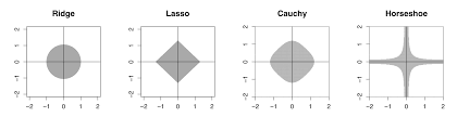
There are a number of commonly used penalty functions (a.k.a. log prior density). For example, the $ l^2$-norm corresponds to s normal prior. The resulting Bayes rule will take the form of a shrinkage estimator, a weighted combination between data and prior beliefs about the parameter. An $ l^1 $-norm will induce a sparse solution in the estimator and can be used an a variable selection operator. The $ l_0 $-norm directly induces a subset selection procedure.

The amount of regularisation $ $ gauges the trade-off between the compromise between the observed data and the initial prior beliefs.

There are two main approaches to finding a good model:

Full Bayes: This approach places a prior distribution on the parameters and computes the full posterior distribution.
Regularization Methods: These approaches add penalty terms to the objective function to control model complexity. Common examples include ridge regression (L2 penalty), lasso regression (L1 penalty), and elastic net (combination of L1 and L2 penalties).

12.2 Normal Means Problem

The canonical problem is estimation in the normal means problem. Suppose that we have $y_i = \theta_i + e_i,~i=1,\ldots,p$ and $e_i \sim N(0, \sigma^2)$. The goal is to estimate the vector of means $\theta = (\theta_1, \ldots, \theta_p)$. This is also a proxy for non-parametric regression, where $\theta_i = f(x_i)$. Also typically $y_i$ is a mean of $n$ observations, i.e. $y_i = \frac{1}{n} \sum_{j=1}^n x_{ij}$. Much has been written on the properties of the Bayes risk as a function of $n$ and $p$. Much work has also been done on the asymptotic properties of the Bayes risk as $n$ and $p$ grow to infinity. We now summarise some of the standard risk results.

12.2.1 James-Stein Estimator

The classic James-Stein shrinkage rule, $\hat \thea_{JS}$, uniformly dominates the traditional sample mean estimator, $\hat{\theta}$, for all values of the true parameter $\theta$. In classical MSE risk terms: \[ R(\hat \theta_{JS}, \theta) \defeq E_{y|\theta} {\Vert \hat \theta_{JS} - \theta \Vert}^2 < p = E_{y|\theta} {\Vert y - \theta \Vert}^2, \;\;\; \forall \theta \]

From a historical perspective, James-Stein (a.k.a $L^2$-regularisation)(Stein 1964) is only a global shrinkage rule–in the sense that there are no local parameters to learn about sparsity. A simple sparsity example shows the issue with $L^2$-regularisation. Consider the sparse $r$-spike shows the problem with focusing solely on rules with the same shrinkage weight (albeit benefiting from pooling of information).

From a risk perspective $E \Vert \hat{\theta}^{JS} - \theta \Vert \leq p , \forall \theta$ showing the inadmissibility of the MLE. At origin the risk is $2$.

12.3 $\ell_2$ Shrinkage

Example 12.1 (Stein’s Paradox) Stein’s paradox, as explained Efron and Morris (1977), is a phenomenon in statistics that challenges our intuitive understanding of estimation. The paradox arises when trying to estimate the mean of a multivariate normal distribution. Traditionally, the best guess about the future is usually obtained by computing the average of past events. However, Charles Stein showed that there are circumstances where there are estimators better than the arithmetic average. This is what’s known as Stein’s paradox.

In 1961, James and Stein exhibited an estimator of the mean of a multivariate normal distribution that has uniformly lower mean squared error than the sample mean. This estimator is reviewed briefly in an empirical Bayes context. Stein’s rule and its generalizations are then applied to predict baseball averages, to estimate toxomosis prevalence rates, and to estimate the exact size of Pearson’s chi-square test with results from a computer simulation.

In each of these examples, the mean square error of these rules is less than half that of the sample mean. This result is paradoxical because it contradicts the elementary law of statistical theory. The philosophical implications of Stein’s paradox are also significant. It has influenced the development of shrinkage estimators and has connections to Bayesianism and model selection criteria.

Suppose that we have $n$ independent observations $y_{1},\ldots,y_{n}$ from a $N\left( \theta,\sigma^{2}\right)$ distribution. The maximum likelihood estimator is $\widehat{\theta}=\bar{y}$, the sample mean. The Bayes estimator is the posterior mean, \[ \widehat{\theta}=\mathbb{E}\left[ \theta\mid y\right] =\frac{\sigma^{2}}{\sigma^{2}+n}% \bar{y}. \] The Bayes estimator is a shrinkage estimator, it shrinks the MLE towards the prior mean. The amount of shrinkage is determined by the ratio of the variance of the prior and the variance of the likelihood. The Bayes estimator is also a function of the MLE \[ \widehat{\theta}=\frac{\sigma^{2}}{\sigma^{2}+n}\bar{y}+\frac{n}{\sigma^{2}+n}\widehat{\theta}. \] This is a general property of Bayes estimators, they are functions of the MLE. This is a consequence of the fact that the posterior distribution is a function of the likelihood and the prior. The Bayes estimator is a function of the MLE \[ \widehat{\theta}=\frac{\sigma^{2}}{\sigma^{2}+n}\bar{y}+\frac{n}{\sigma^{2}+n}\widehat{\theta}. \] This is a general property of Bayes estimators, they are functions of the MLE. This is a consequence of the fact that the posterior distribution is a function of the likelihood and the prior.

The original JS estimator shranks to zero and estimates prior variance using empirical Bayes (marginal MLE or Type II MLE). Efron and Morris and Lindley showed that you want o shrink to overall mean $\bar y$ and in this approach \[ \theta \sim N(\mu,\tau^2). \] The original JS is $\mu=0$. To estimate the $\mu$ and $\tau$ you can do full Bayes or empirical Bayes that shrinks to overall grand mean $\bar y$, which serves as the estimate of the original prior mean $\mu$. It seems paradoxical that you estimate propr from the data. However, this is not the case. You simply use mixture prior Diaconis and Ylvisaker (1983) with marginal MLE (MMLE). The MMLE is the product \[ \int_{\theta_i}\prod_{i=1}^k p(\bar y_i \mid \theta_i)p(\theta_i \mid \mu, \tau^2). \]

12.3.1 Sparse $r$-spike problem

For the sparse $r$-spike problem we require a different rule. For a sparse signal, however, $\hat \theta_{JS}$ performs poorly when the true parameter is an $r$-spike where $\theta_r$ has $r$ coordinates at $\sqrt{p/r}$ and the rest set at zero with norm ${\Vert \theta_r \Vert}^2 =p$.

The classical risk satisfies $R \left ( \hat \theta_{JS} , \theta_r \right ) \geq p/2$ where the simple thresholding rule $\sqrt{2 \ln p}$ performs with risk $\sqrt{\ln p}$ in the $r$-spike sparse case even though it is inadmissible in MSE for a non-sparse signal. Then is due to the fact that for $ _p $ we have \[ \frac{p \Vert \theta \Vert^2}{p + \Vert \theta \Vert^2} \leq R \left ( \hat{\theta}^{JS} , \theta_p \right ) \leq 2 + \frac{p \Vert \theta \Vert^2}{ d + \Vert \theta \Vert^2}. \] This implies that $R \left ( \hat{\theta}^{JS} , \theta_p \right ) \geq (p/2)$. Hence, simple thresholding rule beats James-Stein this with a risk given by $\sqrt{\log p }$. This simple example, shows that the choice of penalty should not be taken for granted as different estimators will have different risk profiles.

A Bayes rule that inherits good MSE properties but also simultaneously provides asymptotic minimax estimation risk for sparse signals. HS estimator uniformly dominates the traditional sample mean estimator in MSE and has good posterior concentration properties for nearly black objects. Specifically, the horseshoe estimator attains asymptotically minimax risk rate \[ \sup_{ \theta \in l_0[p_n] } \; \mathbb{E}_{ y | \theta } \|\hat y_{hs} - \theta \|^2 \asymp p_n \log \left ( n / p_n \right ). \] The “worst’’ $\theta$ is obtained at the maximum difference between $\left| \hat \theta_{HS} - y \right|$ where $\hat \theta_{HS} = \mathbb{E}(\theta|y)$ can be interpreted as a Bayes posterior mean (optimal under Bayes MSE).

One such estimator that achieves the optimal minimax rate is the horseshoe estimator proposed by Carvalho, Polson, and Scott (2010) t

12.3.2 Efron Example

Efron provide an example which shows the importance of specifying priors in high dimensions. The key idea behind James-Stein shrinkage is that one when one can “borrow strength” across components. In this sense the multivariate parameter estimation problem is easier than the univariate one.

Stein’s phenomenon where $y_i | \theta_i \sim N(\theta_i, 1)$ and $\theta_i \sim N(0, \tau^2)$ where $ $ illustrates this point well. This leads to the improper “non-informative” uniform prior. The corresponding generalized Bayes rule is the vector of means—which we know is inadmissible. so no regularisation leads to an estimator with poor risk property.

Let $ || y || = _{i=1}^p y_i^2 $. Then, we can make the following probabilistic statements from the model,$$ P( | y | > | | ) > \[ Now for the posterior, this inequallty is reversed under a flat Lebesgue measure, \] P( | | > | y | ; | ; y ) > $$ which is in conflict with the classical statement. This is a property of the prior which leads to a poor rule (the overall average) and risk.

The shrinkage rule (a.k.a. normal prior) where $ ^2 $ is “estimated” from the data avoids this conflict. More precisely, we have \[ \hat{\theta}(y) = \left( 1 - \frac{k-2}{\|y\|^2} \right) y \quad \text{and} \quad E\left( \| \hat{\theta} - \theta \| \right) < k, \; \forall \theta. \] Hence, when $\|y\|^2$ is small the shrinkage factor is more extreme. For example, if $k=10$, $\|y\|^2=12$, then $\hat{\theta} = (1/3) y$. Now we have the more intuitive result that $ P( | | > | y | ; | ; y ) < $.

This shows that careful specification of default priors matter in high dimensions is necessary.

Example 12.2 (Example: James-Stein for Baseball Batting Averages) We reproduce the baseball batting average example from Efron and Morris (1977). Data below has the number of hits for 18 baseball player after 45 at-beat in 1970 season

# Data source: https://www1.swarthmore.edu/NatSci/peverso1/Sports%20Data/JamesSteinData/Efron-Morris%20Baseball/EfronMorrisBB.txt
baseball = read.csv("../data/EfronMorrisBB.txt", sep = "\t", stringsAsFactors = FALSE) %>% select(LastName,AtBats,BattingAverage,SeasonAverage)

Now, we can eatimate overall mean and variance

mu_hat <- mean(baseball$BattingAverage)
sigma2_hat <- var(baseball$BattingAverage)

As well as the posterior mean for each player (James-Stein estimator)

baseball <- baseball %>%
  mutate(
    JS = (sigma2_hat / (sigma2_hat + (BattingAverage * (1 - BattingAverage) / AtBats))) * mu_hat +
      ((BattingAverage * (1 - BattingAverage) / AtBats) / (sigma2_hat + (BattingAverage * (1 - BattingAverage) / AtBats))) * BattingAverage
  )
kable(baseball)

LastName	AtBats	BattingAverage	SeasonAverage	JS
Clemente	45	0.40	0.35	0.34
Robinson	45	0.38	0.31	0.32
Howard	45	0.36	0.28	0.31
Johnstone	45	0.33	0.24	0.30
Berry	45	0.31	0.28	0.29
Spencer	45	0.31	0.27	0.29
Kessinger	45	0.29	0.27	0.28
Alvarado	45	0.27	0.22	0.27
Santo	45	0.24	0.27	0.26
Swaboda	45	0.24	0.23	0.26
Petrocelli	45	0.22	0.26	0.25
Rodriguez	45	0.22	0.22	0.25
Scott	45	0.22	0.30	0.25
Unser	45	0.22	0.26	0.25
Williams	45	0.22	0.25	0.25
Campaneris	45	0.20	0.28	0.24
Munson	45	0.18	0.30	0.23
Alvis	45	0.16	0.18	0.22

Plot below shows the observed averages vs. James-Stein estimate

ggplot(baseball, aes(x = BattingAverage, y = JS)) +
  geom_point(alpha = 0.6) +
  geom_abline(slope = 1, intercept = 0, linetype = "dashed", color = "red") +
  labs(
    x = "Observed Batting Average",
    y = "James-Stein Estimate",
    title = "Empirical Bayes Shrinkage of Batting Averages (2016)"
  )

Calculate mean squared error (MSE) for observed and James-Stein estimates

mse_observed <- mean((baseball$BattingAverage - mu_hat)^2)
mse_js <- mean((baseball$JS - mu_hat)^2)

cat(sprintf("MSE (Observed): %.6f\n", mse_observed))

MSE (Observed): 0.004584

cat(sprintf("MSE (James-Stein): %.6f\n", mse_js))

MSE (James-Stein): 0.001031

We can see that the James-Stein estimator has a lower MSE than the observed batting averages. This is a demonstration of Stein’s paradox, where the James-Stein estimator, which shrinks the estimates towards the overall mean, performs better than the naive sample mean estimator.

a = matrix(rep(1:3, nrow(baseball)), 3, nrow(baseball))
b = matrix(c(baseball$BattingAverage, baseball$SeasonAverage, baseball$JS),    3, nrow(baseball), byrow=TRUE)

matplot(a, b, pch=" ", ylab="predicted average", xaxt="n", xlim=c(0.5, 3.1), ylim=c(0.13, 0.42))
matlines(a, b)
text(rep(0.7, nrow(baseball)), baseball$BattingAverage, baseball$LastName, cex=0.6)
text(1, 0.14, "First 45\nat bats", cex=0.5)
text(2, 0.14, "Average\nof remainder", cex=0.5)
text(3, 0.14, "J-S\nestimator", cex=0.5)

Now if we look at the season dynamics for Clemente

# Data source: https://www.baseball-almanac.com/players/hittinglogs.php?p=clemero01&y=1970
cl = read.csv("../data/clemente.csv")
x = cumsum(cl$AB)
y = cumsum(cl$H)/cumsum(cl$AB)
# Plot x,y startind from index 2
ind = c(1,2)
plot(x[-ind],y[-ind], type='o', ylab="Betting Average", xlab="Number at Bats")
# Add horizontal line for season average 145/412 and add text above line `Seaosn Average`
text(200, 145/412 + 0.005, "Season Average", col = "red")
abline(h = 145/412, col = "red", lty = 2)
# Ted williams record is .406 in in 1941, so you know the first data points are noise
text(200, baseball$JS[1] + 0.005, "JS", col = "red")
abline(h = baseball$JS[1], col = "red", lty = 2)
text(200, baseball$BattingAverage[1] + 0.005, "After 45 Bets", col = "red")
abline(h = baseball$BattingAverage[1], col = "red", lty = 2)

The motivation for the shrinkage prior rather than a flat uniform prior are the following probabilistic arguments.

12.4 $\ell_1$ Sparsity

12.5 $\ell_0$ Subset Selection

The canonical problem is estimaiton of the normal means problem. Here we have $y_i = \theta_i + e_i,~i=1,\ldots,p$ and $e_i \sim N(0, \sigma^2)$. The goal is to estimate the vector of means $\theta = (\theta_1, \ldots, \theta_p)$. This is also a proxy for non-parametric regression, where $\theta_i = f(x_i)$. Aslo typically $y_i$ is a mean of $n$ observations, i.e. $y_i = \frac{1}{n} \sum_{j=1}^n x_{ij}$. Much has been written on the properties of the Bayes risk as a function of $n$ and $p$. Much work has also been done on the asymptotic properties of the Bayes risk as $n$ and $p$ grow to infinity. We now sumamrise some of the standard risk results.

12.6 James-Stein Estimator

The classic James-Stein shrinkage rule, $\hat y_{js}$, uniformly dominates the traditional sample mean estimator, $\hat{\theta}$, for all values of the true parameter $\theta$. In classical MSE risk terms: \[ R(\hat y_{js}, \theta) \defeq E_{y|\theta} {\Vert \hat y_{js} - \theta \Vert}^2 < p = E_{y|\theta} {\Vert y - \theta \Vert}^2, \;\;\; \forall \theta \] For a sparse signal, however, $\hat y_{js}$ performs poorly when the true parameter is an $r$-spike where $\theta_r$ has $r$ coordinates at $\sqrt{p/r}$ and the rest set at zero with norm ${\Vert \theta_r \Vert}^2 =p$.

The classical risk satisfies $R \left ( \hat y_{js} , \theta_r \right ) \geq p/2$ where the simple thresholding rule $\sqrt{2 \ln p}$ performs with risk $\sqrt{\ln p}$ in the $r$-spike sparse case even though it is inadmissible in MSE for a non-sparse signal.

12.7 R-spike Problem

Let the true parameter value be $\theta_p = \left ( \sqrt{d/p} , \ldots , \sqrt{d/p} , 0 , \ldots , 0 \right )$. James-Stein is equivalent to the model \[ y_i = \theta_i + \epsilon_i \; \mathrm{ and} \; \theta_i \sim \mathcal{N} \left ( 0 , \tau^2 \right ) \] This dominates the plain MLE but loses admissibility! This is due to the fact that a “plug-in” estimate of global shrinkage $\hat{\tau}$ is used. Tiao and Tan’s original “closed-form” analysis is particularly relevant here. They point out that the mode of $p(\tau^2|y)$ is zero exactly when the shrinkage weight turns negative (their condition 6.6). From a risk perspective $E \Vert \hat{\theta}^{JS} - \theta \Vert \leq p , \forall \theta$ showing the inadmissibility of the MLE. At origin the risk is $2$, but! \[ \frac{p \Vert \theta \Vert^2}{p + \Vert \theta \Vert^2} \leq R \left ( \hat{\theta}^{JS} , \theta_p \right ) \leq 2 + \frac{p \Vert \theta \Vert^2}{ d + \Vert \theta \Vert^2}. \] This implies that $R \left ( \hat{\theta}^{JS} , \theta_p \right ) \geq (p/2)$. Hence, simple thresholding rule beats James-Stein this with a risk given by $\sqrt{\log p }$. This simple example, shows that the choice of penalty should not be taken for granted as different estimators will have different risk profiles.

The horseshoe estimator, which we will discuss in more detail later, $\hat y_{hs}$, was proposed by Carvalho, Polson, and Scott (2010) to provide a Bayes rule that inherits good MSE properties but also simultaneously provides asymptotic minimax estimation risk for sparse signals. HS estimator uniformly dominates the traditional sample mean estimator in MSE and has good posterior concentration properties for nearly black objects. Specifically, the horseshoe estimator attains asymptotically minimax risk rate \[ \sup_{ \theta \in l_0[p_n] } \; \mathbb{E}_{ y | \theta } \|\hat y_{hs} - \theta \|^2 \asymp p_n \log \left ( n / p_n \right ). \] The “worst’’ $\theta$ is obtained at the maximum difference between $\left| \hat y_{hs} - y \right|$ where $\hat y_{hs} = \mathbb{E}(\theta|y)$ can be interpreted as a Bayes posterior mean (optimal under Bayes MSE).

12.8 $\ell_2$ Shrinkage

Example 12.3 (Stein’s Paradox) Stein’s paradox, as explained Efron and Morris (1977), is a phenomenon in statistics that challenges our intuitive understanding of estimation. The paradox arises when trying to estimate the mean of a multivariate normal distribution. Traditionally, the best guess about the future is usually obtained by computing the average of past events. However, Charles Stein showed that there are circumstances where there are estimators better than the arithmetic average. This is what’s known as Stein’s paradox.

The original JS estimator shranks to zero and estimates prior variance using empirical Bayes (marginal MLE or Type II MLE). Efron and MOrris and Lindley showed that you want o shrink to overall mean $\bar y$ and in this approach \[ \theta \sim N(\mu,\tau^2). \] The original JS is $\mu=0$. To estimate the $\mu$ and $\tau$ you can do full Bayes or empirical Bayes that shrinks to overall grand mean $\bar y$, whcih serves as the estimate of the original prior mean $\mu$. It seems paradoxical that you estimate propr from the data. However, this is not the case. You simply use mixture prior Diaconis and Ylvisaker (1983) with marginal MLE (MMLE). The MMLE is the product \[ \int_{\theta_i}\prod_{i=1}^k p(\bar y_i \mid \theta_i)p(\theta_i \mid \mu, \tau^2). \]

We reproduce the baseball bartting average example from Efron and Morris (1977). Data below has the number of hits for 18 baseball player after 45 at-beat in 1970 season

# Data source: https://www1.swarthmore.edu/NatSci/peverso1/Sports%20Data/JamesSteinData/Efron-Morris%20Baseball/EfronMorrisBB.txt
baseball = read.csv("../data/EfronMorrisBB.txt", sep = "\t", stringsAsFactors = FALSE) %>% select(LastName,AtBats,BattingAverage,SeasonAverage)

Now, we can eatimate overall mean and variance

mu_hat <- mean(baseball$BattingAverage)
sigma2_hat <- var(baseball$BattingAverage)

As well as the osterior mean for each player (James-Stein estimator)

baseball <- baseball %>%
  mutate(
    JS = (sigma2_hat / (sigma2_hat + (BattingAverage * (1 - BattingAverage) / AtBats))) * mu_hat +
      ((BattingAverage * (1 - BattingAverage) / AtBats) / (sigma2_hat + (BattingAverage * (1 - BattingAverage) / AtBats))) * BattingAverage
  )
kable(baseball)

LastName	AtBats	BattingAverage	SeasonAverage	JS
Clemente	45	0.40	0.35	0.34
Robinson	45	0.38	0.31	0.32
Howard	45	0.36	0.28	0.31
Johnstone	45	0.33	0.24	0.30
Berry	45	0.31	0.28	0.29
Spencer	45	0.31	0.27	0.29
Kessinger	45	0.29	0.27	0.28
Alvarado	45	0.27	0.22	0.27
Santo	45	0.24	0.27	0.26
Swaboda	45	0.24	0.23	0.26
Petrocelli	45	0.22	0.26	0.25
Rodriguez	45	0.22	0.22	0.25
Scott	45	0.22	0.30	0.25
Unser	45	0.22	0.26	0.25
Williams	45	0.22	0.25	0.25
Campaneris	45	0.20	0.28	0.24
Munson	45	0.18	0.30	0.23
Alvis	45	0.16	0.18	0.22

Plot below shows the observed averages vs. James-Stein estimate

ggplot(baseball, aes(x = BattingAverage, y = JS)) +
  geom_point(alpha = 0.6) +
  geom_abline(slope = 1, intercept = 0, linetype = "dashed", color = "red") +
  labs(
    x = "Observed Batting Average",
    y = "James-Stein Estimate",
    title = "Empirical Bayes Shrinkage of Batting Averages (2016)"
  )

Calculate mean squared error (MSE) for observed and James-Stein estimates

mse_observed <- mean((baseball$BattingAverage - mu_hat)^2)
mse_js <- mean((baseball$JS - mu_hat)^2)

cat(sprintf("MSE (Observed): %.6f\n", mse_observed))

MSE (Observed): 0.004584

cat(sprintf("MSE (James-Stein): %.6f\n", mse_js))

MSE (James-Stein): 0.001031

a = matrix(rep(1:3, nrow(baseball)), 3, nrow(baseball))
b = matrix(c(baseball$BattingAverage, baseball$SeasonAverage, baseball$JS),    3, nrow(baseball), byrow=TRUE)

matplot(a, b, pch=" ", ylab="predicted average", xaxt="n", xlim=c(0.5, 3.1), ylim=c(0.13, 0.42))
matlines(a, b)
text(rep(0.7, nrow(baseball)), baseball$BattingAverage, baseball$LastName, cex=0.6)
text(1, 0.14, "First 45\nat bats", cex=0.5)
text(2, 0.14, "Average\nof remainder", cex=0.5)
text(3, 0.14, "J-S\nestimator", cex=0.5)

Now if we look at the season dynamics for Clemente

# Data source: https://www.baseball-almanac.com/players/hittinglogs.php?p=clemero01&y=1970
cl = read.csv("../data/clemente.csv")
x = cumsum(cl$AB)
y = cumsum(cl$H)/cumsum(cl$AB)
# Plot x,y startind from index 2
ind = c(1,2)
plot(x[-ind],y[-ind], type='o', ylab="Betting Average", xlab="Number at Bats")
# Add horizontal line for season average 145/412 and add text above line `Seaosn Average`
text(200, 145/412 + 0.005, "Season Average", col = "red")
abline(h = 145/412, col = "red", lty = 2)
# Ted williams record is .406 in in 1941, so you know the first data points are noise
text(200, baseball$JS[1] + 0.005, "JS", col = "red")
abline(h = baseball$JS[1], col = "red", lty = 2)
text(200, baseball$BattingAverage[1] + 0.005, "After 45 Bets", col = "red")
abline(h = baseball$BattingAverage[1], col = "red", lty = 2)

The motivation for the shrinkage prior rather than a flat uniform prior are the following probabilistic arguments.

Example 12.4 (Efron Example) Efron shows the importance of priors in high dimensions when one can “borrow strength” (a.k.a. regularisation) across components.

Stein’s phenomenon where $y_i | \theta_i \sim N(\theta_i, 1)$ and $\theta_i \sim N(0, \tau^2)$ illustrates this point well. From the model,

\[ P\left( \| y \| > \| \theta \| \right) > \frac{1}{2} \]

Under a flat Lebesgue measure, this inequality is reversed in the posterior, namely

\[ P\left( \| \theta \| > \| y \| \; | \; y \right) > \frac{1}{2} \]

In conflict with the classical statement. However, if we use Stein’s rule (posterior where $\tau^2$ is estimated via empirical Bayes) we have

\[ \hat{\theta}(y) = \left( 1 - \frac{k-2}{\|y\|^2} \right) y \quad \text{and} \quad E\left( \| \hat{\theta} - \theta \| \right) < k, \; \forall \theta. \]

Hence, when $\|y\|^2$ is small the shrinkage factor is more extreme.

For example, if $k=10$, $\|y\|^2=12$, then $\hat{\theta} = (1/3) y$. Now we have the more intuitive result:

\[ P\left( \| \theta \| > \| y \| \; | \; y \right) < \frac{1}{2} \]

Showing that default priors matter in high dimensions.

12.9 $\ell_1$ Sparsity

12.10 $\ell_0$ Subset Selection

12.11 Bayesain Model Selection via Regularisation

From Bayesian perspective regularization is nothing but incorporation of prior information into the model. Remember, that a Bayesian model is specified by likelihood and prior distributions. Bayesian regularization methods include the Bayesian bridge, horseshoe regularization, Bayesian lasso, Bayesian elastic net, spike-and-slab lasso, and global-local shrinkage priors. Bayesian $\ell_0$ regularization is an attractive solution for high dimensional variable selection as it directly penalizes the number of predictors. The caveat is the need to search over all possible model combinations, as a full solution requires enumeration over all possible models which is NP-hard.

In Bayesian approach, regularization requires the specification of a loss, denoted by $l\left(\beta\right)$ and a penalty function, denoted by $\phi_{\lambda}(\beta)$, where $\lambda$ is a global regularization parameter. From a Bayesian perspective, $l\left(\beta\right)$ and $\phi_{\lambda}(\beta)$ correspond to the negative logarithms of the likelihood and prior distribution, respectively. Regularization leads to an maximum a posteriori (MAP) optimization problem of the form \[ \underset{\beta \in R^p}{\mathrm{minimize}\quad} l\left(\beta\right) + \phi_{\lambda}(\beta) \; . \] Taking a probabilistic approach leads to a Bayesian hierarchical model \[ p(y \mid \beta) \propto \exp\{-l(\beta)\} \; , \quad p(\beta) \propto \exp\{ -\phi_{\lambda}(\beta) \} \ . \] The solution to the minimization problem estimated by regularization corresponds to the posterior mode, $\hat{\beta} = \mathrm{ arg \; max}_\beta \; p( \beta|y)$, where $p(\beta|y)$ denotes the posterior distribution. Consider a normal mean problem with \[ \label{eqn:linreg} y = \theta+ e \ , \ \ \text{where } e \sim N(0, \sigma^2),~-\infty \le \theta \le \infty \ . \] What prior $p(\theta)$ should we place on $\theta$ to be able to separate the “signal” $\theta$ from “noise” $e$, when we know that there is a good chance that $\theta$ is sparse (i.e. equal to zero). In the multivariate case we have $y_i = \theta_i + e_i$ and sparseness is measured by the number of zeros in $\theta = (\theta_1\ldots,\theta_p)$. The Bayesan Lasso assumes double exponential (a.k.a Laplace) prior distribution where \[ p(\theta_i \mid b) = 0.5b\exp(-|\theta|/b). \] We use Bayes rule to calculate the posterior as a product of Normal likelihood and Laplace prior \[ \log p(\theta \mid y, b) \propto ||y-\theta||_2^2 + \dfrac{2\sigma^2}{b}||\theta||_1. \] For fixed $\sigma^2$ and $b>0$ the posterior mode is equivalent to the Lasso estimate with $\lambda = 2\sigma^2/b$. Large variance $b$ of the prior is equivalent to the small penalty weight $\lambda$ in the Lasso objective function.

There is a duality between using regularization term in optimisation problem and assuming a prior distribution over the parameters of the model $f$. The regularization parameter $\lambda$ is related to the variance of the prior distribution. When $\lambda=0$, the function $f$ is the maximum likelihood estimate of the parameters. When $\lambda$ is large, the function $f$ is the prior mean of the parameters. When $\lambda$ is infinite, the function $f$ is the prior mode of the parameters. When $\lambda$ is negative, the function $f$ is the posterior mean of the parameters. When $\lambda$ is very negative, the function $f$ is the posterior mode of the parameters.

The goal is to find a function $f$ that minimizes the risk $R(f)$. This is called the empirical risk minimization problem. Finding minimum is a difficult problem when the risk function $R(f)$ is non-convex. In practice, we often use gradient descent to find a local minimum of the risk function $R(f)$.

There are multiple ways to choose the penalty term $\phi(f)$. Sections below describe the most popular approaches.

12.12 Shrinkage ($\ell_2$ Norm)

We can estimate the risk bounds of $\ell_2$ Norm regularisation. The classic bias-variance tradeoff is given by the MSE risk bound. \[ R(\theta,\hat \theta) = E_{y|\theta} \left [ \Vert \hat \theta - \theta \Vert^2 \right ] = \Vert \hat \theta - \theta \Vert^2 + E_{y|\theta} \left [ \Vert \hat \theta - \mathbb{E}(\hat \theta) \Vert^2 \right ] \]

In a case of multiple parameters, the Stein bound is \[ R(\theta,\hat \theta_{JS}) < R(\theta,\hat \theta_{MLE}) \;\;\; \forall \theta \in \mathbb{R}^p, \;\;\; p \geq 3. \] In an applied problem the gap in risk between MLE and JS estimators can be large. For example, in the normal means problem with $p=100$ and $n=100$, the risk of the MLE is $R(\theta,\hat \theta_{MLE}) = 100$ while the risk of the JS estimator is $R(\theta,\hat \theta_{JS}) = 1.5$. The JS estimator is 67 times more efficient than the MLE. The JS estimator is also minimax optimal in the sense that it attains the minimax risk bound for the normal means problem. The minimax risk bound is the smallest risk that can be attained by any estimator.

JS is a specific estimate and it motivates the ridge estimator. The ridge estimator is a shrinkage estimator with the penalty function being the squared norm of the parameter vector. The ridge estimator is \[ \hat \theta_{ridge} = \left ( X^T X + \lambda I \right )^{-1} X^T y \] where $\lambda$ is the regularization parameter.

12.13 Sparsity ($\ell_1$ Norm)

High-dimensional predictor selection and sparse signal recovery are routine statistical and machine learning tasks. There is a vast and growing literator with lasso (leat absolute selection) being the gold standard. Horseshoe priors are the Bayesian counterpart. Sparsity relies on the property of a few large signals among many (nearly zero) noisy observations. The goal is to find a niddle in the haystack. Suppose that we observe data from Normal means model \[ y_i \mid \theta_i \sim N(\theta_i,1),~ 1\le i\le p, ~ \theta = (\theta_1,\ldots,\theta_p), \] where parameter $\theta$ lies in the ball \[ ||\theta||_{\ell_0} = \{\theta : \text{number of }\theta_i \ne 0 \le p_n\}. \]

Even threshholding can beat MLE, when the signal is sparse. The thresholding estimator is \[ \hat \theta_{thr} = \left \{ \begin{array}{ll} \hat \theta_i & \mbox{if} \; \hat \theta_i > \sqrt{2 \ln p} \\ 0 & \mbox{otherwise} \end{array} \right . \]

Sparse signal detection provides a challenge to statistical methodology; consider the classical normal means inference problem. Suppose that we observe data from the probability model $( y_i | \theta_i ) \sim N( \theta_i,1)$. We wish to provide an estimator $\hat y_{hs}$ for the vector of normal means $\theta = ( \theta_1, \ldots , \theta_p )$. Sparsity occurs when a large portion of the parameter vector contains zeroes. The ’’ultra-sparse`` or “nearly black” vector case occurs when $p_n$, denoting the number of non-zero parameter values, and for $\theta \in l_0 [ p_n]$, which denotes the set $\# ( \theta_i \neq 0 ) \leq p_n$ where $p_n = o(n)$ where $p_n \rightarrow \infty$ as $n \rightarrow \infty$.

The predictive rule is often represented by a mathematical model, such as a linear regression model or a neural network. The model is trained using historical data, which consists of observed inputs and outputs $(x_1,y_1),\ldots, (x_n,y_n)$.

The model is then used to predict the output $y$ for new inputs $x$. The accuracy of the model is evaluated using a performance metric, such as the mean squared error or the mean absolute error. The model is then updated and retrained using new data to improve its accuracy. This process is repeated until the model achieves the desired level of accuracy.

12.14 LASSO

The Laplace distribution can be represented as scale mixture of Normal distribution(Andrews and Mallows 1974) \[ \begin{aligned} \theta_i \mid \sigma^2,\tau \sim &N(0,\tau^2\sigma^2)\\ \tau^2 \mid \alpha \sim &\exp (\alpha^2/2)\\ \sigma^2 \sim & \pi(\sigma^2).\end{aligned} \] We can show equivalence by integrating out $\tau$ \[ p(\theta_i\mid \sigma^2,\alpha) = \int_{0}^{\infty} \dfrac{1}{\sqrt{2\pi \tau}}\exp\left(-\dfrac{\theta_i^2}{2\sigma^2\tau}\right)\dfrac{\alpha^2}{2}\exp\left(-\dfrac{\alpha^2\tau}{2}\right)d\tau = \dfrac{\alpha}{2\sigma}\exp(-\alpha/\sigma|\theta_i|). \] Thus it is a Laplace distribution with location 0 and scale $\alpha/\sigma$. Representation of Laplace prior is a scale Normal mixture allows us to apply an efficient numerical algorithm for computing samples from the posterior distribution. This algorithms is called a Gibbs sample and it iteratively samples from $\theta \mid a,y$ and $b\mid \theta,y$ to estimate joint distribution over $(\hat \theta, \hat b)$. Thus, we so not need to apply cross-validation to find optimal value of $b$, the Bayesian algorithm does it “automatically”. We will discuss Gibbs algorithm later in the book.

When prior is Normal $\theta_i \sim N(0,\sigma_{\theta}^2)$, the posterior mode is equivalent to the ridge estimate. The relation between variance of the prior and the penalty weight in ridge regression is inverse proportional $\lambda\propto 1/\sigma_{\theta}^2$.

12.15 Subset Selection ($\ell_0$ Norm)

Skike-and-slab (George and McCulloh) or Bernoulli-Gaussian (Polson Sun)

12.16 Bridge ($\ell_{\alpha}$)

This is a non-convex penalty when $0<\alpha<1$. It is an NP-hard problem. When $\alpha=1$ or $\alpha=2$ we have optimisation problems that are “solvable” for large scale cases. However, when $0\le \alpha<1$ the current optimisation algorithms won’t work.

The real killer is that you can use data to estimate $\alpha$ and $\lambda$ (let the data speak for itself) Box and Tiao (1992).

Bayesian analogue of the bridge estimator in regression is \[ y = X\beta + \epsilon \]

for some unknown vector $\beta = (\beta_1, \ldots, \beta_p)'$. Given choices of $\alpha \in (0,1]$ and $\nu \in \mathbb{R}^+$, the bridge estimator $\hat{\beta}$ is the minimizer of

\[ Q_y(\beta) = \frac{1}{2} \|y - X\beta\|^2 + \nu \sum_{j=1}^p |\beta_j|^\alpha. \tag{12.1}\]

This bridges a class of shrinkage and selection operators, with the best-subset-selection penalty at one end, and the $\ell_1$ (or lasso) penalty at the other. An early reference to this class of models can be found in Frank and Friedman (1993), with recent papers focusing on model-selection asymptotics, along with strategies for actually computing the estimator (Huang, Horowitz, and Ma (2008), Mazumder, and and Hastie (2011)).

Bridge approach differs from this line of work in adopting a Bayesian perspective on bridge estimation. Specifically, we treat

\[ p(\beta \mid y) \propto \exp\{-Q_y(\beta)\} \]

as a posterior distribution having the minimizer of Equation 12.1 as its global mode. This posterior arises in assuming a Gaussian likelihood for $y$, along with a prior for $\beta$ that decomposes as a product of independent exponential-power priors (Box and Tiao (1992)):

\[ p(\beta \mid \alpha, \nu) \propto \prod_{j=1}^p \exp\left(-\left|\frac{\beta_j}{\tau}\right|^\alpha\right), \quad \tau = \nu^{-1/\alpha}. \tag{2} \]

Rather than minimizing (1), we proceed by constructing a Markov chain having the joint posterior for $\beta$ as its stationary distribution.

12.16.1 Spike-and-Slab Prior

Our Bayesian formulation of allows to specify a wide range of range of regularized formulations for a regression problem. In this section we consider a Bayesian model for variable selection. Consider a linear regression problem \[ y = \beta_1x_1+\ldots+\beta_px_p + e \ , \ \ \text{where } e \sim N(0, \sigma^2),~-\infty \le \beta_i \le \infty \ . \] We would like to solve the problem of variable selections, i.e. identify which input variables $x_i$ to be used in our model. The gold standard for Bayesian variable selection are spike-and-slab priors, or Bernoulli-Gaussian mixtures. Whilst spike-and-slab priors provide full model uncertainty quantification, they can be hard to scale to very high dimensional problems and can have poor sparsity properties. On the other hand, techniques like proximal algorithms can solve non-convex optimization problems which are fast and scalable, although they generally don’t provide a full assessment of model uncertainty.

To perform a model selection, we would like to specify a prior distribution $p\left(\beta\right)$, which imposes a sparsity assumption on $\beta$, where only a small portion of all $\beta_i$’s are non-zero. In other words, $\|\beta\|_0 = k \ll p$, where $\|\beta\|_0 \defeq \#\{i : \beta_i\neq0\}$, the cardinality of the support of $\beta$, also known as the $\ell_0$ (pseudo)norm of $\beta$. A multivariate Gaussian prior ($l_2$ norm) leads to poor sparsity properties in this situation. Sparsity-inducing prior distributions for $\beta$ can be constructed to impose sparsity include the double exponential (lasso).

Under spike-and-slab, each $\beta_i$ exchangeably follows a mixture prior consisting of $\delta_0$, a point mass at $0$, and a Gaussian distribution centered at zero. Hence we write,

\[ \label{eqn:ss} \beta_i | \theta, \sigma_\beta^2 \sim (1-\theta)\delta_0 + \theta N\left(0, \sigma_\beta^2\right) \ . \] Here $\theta\in \left(0, 1\right)$ controls the overall sparsity in $\beta$ and $\sigma_\beta^2$ accommodates non-zero signals. This family is termed as the Bernoulli-Gaussian mixture model in the signal processing community.

A useful re-parameterization, the parameters $\beta$ is given by two independent random variable vectors $\gamma = \left(\gamma_1, \ldots, \gamma_p\right)'$ and $\alpha = \left(\alpha_1, \ldots, \alpha_p\right)'$ such that $\beta_i = \gamma_i\alpha_i$, with probabilistic structure \[ \label{eq:bg} \begin{array}{rcl} \gamma_i\mid\theta & \sim & \text{Bernoulli}(\theta) \ ; \\ \alpha_i \mid \sigma_\beta^2 &\sim & N\left(0, \sigma_\beta^2\right) \ . \\ \end{array} \] Since $\gamma_i$ and $\alpha_i$ are independent, the joint prior density becomes \[ p\left(\gamma_i, \alpha_i \mid \theta, \sigma_\beta^2\right) = \theta^{\gamma_i}\left(1-\theta\right)^{1-\gamma_i}\frac{1}{\sqrt{2\pi}\sigma_\beta}\exp\left\{-\frac{\alpha_i^2}{2\sigma_\beta^2}\right\} \ , \ \ \ \text{for } 1\leq i\leq p \ . \] The indicator $\gamma_i\in \{0, 1\}$ can be viewed as a dummy variable to indicate whether $\beta_i$ is included in the model.

Let $S = \{i: \gamma_i = 1\} \subseteq \{1, \ldots, p\}$ be the “active set" of $\gamma$, and $\|\gamma\|_0 = \sum\limits_{i = 1}^p\gamma_i$ be its cardinality. The joint prior on the vector $\{\gamma, \alpha\}$ then factorizes as \[ \begin{array}{rcl} p\left(\gamma, \alpha \mid \theta, \sigma_\beta^2\right) & = & \prod\limits_{i = 1}^p p\left(\alpha_i, \gamma_i \mid \theta, \sigma_\beta^2\right) \\ & = & \theta^{\|\gamma\|_0} \left(1-\theta\right)^{p - \|\gamma\|_0} \left(2\pi\sigma_\beta^2\right)^{-\frac p2}\exp\left\{-\frac1{2\sigma_\beta^2}\sum\limits_{i = 1}^p\alpha_i^2\right\} \ . \end{array} \]

Let $X_\gamma \defeq \left[X_i\right]_{i \in S}$ be the set of “active explanatory variables" and $\alpha_\gamma \defeq \left(\alpha_i\right)'_{i \in S}$ be their corresponding coefficients. We can write $X\beta = X_\gamma \alpha_\gamma$. The likelihood can be expressed in terms of $\gamma$, $\alpha$ as \[ p\left(y \mid \gamma, \alpha, \theta, \sigma_e^2\right) = \left(2\pi\sigma_e^2\right)^{-\frac n2} \exp\left\{ -\frac1{2\sigma_e^2}\left\|y - X_\gamma \alpha_\gamma\right\|_2^2 \right\} \ . \]

Under this re-parameterization by $\left\{\gamma, \alpha\right\}$, the posterior is given by

\[ \begin{array}{rcl} p\left(\gamma, \alpha \mid \theta, \sigma_\beta^2, \sigma_e^2, y\right) & \propto & p\left(\gamma, \alpha \mid \theta, \sigma_\beta^2\right) p\left(y \mid \gamma, \alpha, \theta, \sigma_e^2\right)\\ & \propto & \exp\left\{-\frac1{2\sigma_e^2}\left\|y - X_\gamma \alpha_\gamma\right\|_2^2 -\frac1{2\sigma_\beta^2}\left\|\alpha\right\|_2^2 -\log\left(\frac{1-\theta}{\theta}\right) \left\|\gamma\right\|_0 \right\} \ . \end{array} \] Our goal then is to find the regularized maximum a posterior (MAP) estimator \[ \arg\max\limits_{\gamma, \alpha}p\left(\gamma, \alpha \mid \theta, \sigma_\beta^2, \sigma_e^2, y \right) \ . \] By construction, the $\gamma$ $\in\left\{0, 1\right\}^p$ will directly perform variable selection. Spike-and-slab priors, on the other hand, will sample the full posterior and calculate the posterior probability of variable inclusion. Finding the MAP estimator is equivalent to minimizing over $\left\{\gamma, \alpha\right\}$ the regularized least squares objective function

\[ \min\limits_{\gamma, \alpha}\left\|y - X_\gamma \alpha_\gamma\right\|_2^2 + \frac{\sigma_e^2}{\sigma_\beta^2}\left\|\alpha\right\|_2^2 + 2\sigma_e^2\log\left(\frac{1-\theta}{\theta}\right) \left\|\gamma\right\|_0 \ . \tag{12.2}\] This objective possesses several interesting properties:

The first term is essentially the least squares loss function.
The second term looks like a ridge regression penalty and has connection with the signal-to-noise ratio (SNR) $\sigma_\beta^2/\sigma_e^2$. Smaller SNR will be more likely to shrink the estimates towards $0$. If $\sigma_\beta^2 \gg \sigma_e^2$, the prior uncertainty on the size of non-zero coefficients is much larger than the noise level, that is, the SNR is sufficiently large, this term can be ignored. This is a common assumption in spike-and-slab framework in that people usually want $\sigma_\beta \to \infty$ or to be “sufficiently large" in order to avoid imposing harsh shrinkage to non-zero signals.
If we further assume that $\theta < \frac12$, meaning that the coefficients are known to be sparse a priori, then $\log\left(\left(1-\theta\right) / \theta\right) > 0$, and the third term can be seen as an $\ell_0$ regularization.

Therefore, our Bayesian objective inference is connected to $\ell_0$-regularized least squares, which we summarize in the following proposition.

(Spike-and-slab MAP & $\ell_0$ regularization)

For some $\lambda > 0$, assuming $\theta < \frac12$, $\sigma_\beta^2 \gg \sigma_e^2$, the Bayesian MAP estimate defined by Equation 12.2 is equivalent to the $\ell_0$ regularized least squares objective, for some $\lambda > 0$, \[ \min\limits_{\beta} \frac12\left\|y - X\beta\right\|_2^2 + \lambda \left\|\beta\right\|_0 \ . \tag{12.3}\]

First, assuming that \[ \theta < \frac12, \ \ \ \sigma_\beta^2 \gg \sigma_e^2, \ \ \ \frac{\sigma_e^2}{\sigma_\beta^2}\left\|\alpha\right\|_2^2 \to 0 \ , \] gives us an objective function of the form \[ \min\limits_{\gamma, \alpha} \frac12 \left\|y - X_\gamma \alpha_\gamma\right\|_2^2 + \lambda \left\|\gamma\right\|_0, \ \ \ \ \text{where } \lambda \defeq \sigma_e^2\log\left(\left(1-\theta\right) / \theta\right) > 0 \ . \tag{12.4}\]

Equation Equation 12.4 can be seen as a variable selection version of equation Equation 12.3. The interesting fact is that Equation 12.3 and Equation 12.4 are equivalent. To show this, we need only to check that the optimal solution to Equation 12.3 corresponds to a feasible solution to Equation 12.4 and vice versa. This is explained as follows.

On the one hand, assuming $\hat\beta$ is an optimal solution to Equation 12.3, then we can correspondingly define $\hat\gamma_i \defeq I\left\{\hat\beta_i \neq 0\right\}$, $\hat\alpha_i \defeq \hat\beta_i$, such that $\left\{\hat\gamma, \hat\alpha\right\}$ is feasible to Equation 12.4 and gives the same objective value as $\hat\beta$ gives Equation 12.3.

On the other hand, assuming $\left\{\hat\gamma, \hat\alpha\right\}$ is optimal to Equation 12.4, implies that we must have all of the elements in $\hat\alpha_\gamma$ should be non-zero, otherwise a new $\tilde\gamma_i \defeq I\left\{\hat\alpha_i \neq 0\right\}$ will give a lower objective value of Equation 12.4. As a result, if we define $\hat\beta_i \defeq \hat\gamma_i\hat\alpha_i$, $\hat\beta$ will be feasible to Equation 12.3 and gives the same objective value as $\left\{\hat\gamma, \hat\alpha\right\}$ gives Equation 12.4.

12.17 Horseshoe Prior

The sparse normal means problem is concerned with inference for the parameter vector $\theta = ( \theta_1 , \ldots , \theta_p )$ where we observe data $y_i = \theta_i + \epsilon_i$ where the level of sparsity might be unknown. From both a theoretical and empirical viewpoint, regularized estimators have won the day. This still leaves open the question of how does specify a penalty, denoted by $\pi_{HS}$, (a.k.a. log-prior, $- \log p_{HS}$)? Lasso simply uses an $L^1$-norm, $\sum_{i=1}^K | \theta_i |$, as opposed to the horseshoe prior which (essentially) uses the penalty \[ \pi_{HS} ( \theta_i | \tau ) = - \log p_{HS} ( \theta_i | \tau ) = - \log \log \left ( 1 + \frac{2 \tau^2}{\theta_i^2} \right ) . \] The motivation for the horseshoe penalty arises from the analysis of the prior mass and influence on the posterior in both the tail and behaviour at the origin. The latter is the key determinate of the sparsity properties of the estimator.

The horseshoe Carvalho, Polson, and Scott (2010) is a Bayesian method for ‘needle-in-a-haystack’ type problems where there is some sparsity, meaning that there are some signals amid mostly noise.

We introduce the horseshoe in the context of the normal means model, which is given by \[Y_i = \beta_i + \varepsilon_i, \quad i = 1, \ldots, n,\] with $\varepsilon_i$ i.i.d. $\mathcal{N}(0, \sigma^2)$. The horseshoe prior is given by \[\begin{align*} \beta_i &\sim \mathcal{N}(0, \sigma^2 \tau^2 \lambda_i^2)\\ \lambda_i &\sim C^+(0, 1), \end{align*}\] where $C^+$ denotes the half-Cauchy distribution. Optionally, hyperpriors on $\tau$ and $\sigma$ may be specified, as is described further in the next two sections.

To illustrate the shrinkage behaviour of the horseshoe, let’s plot the posterior mean for $\beta_i$ as a function of $y_i$ for three different values of $\tau$.

library(horseshoe)
library(ggplot2)
tau.values <- c(0.005, 0.05, 0.5)
y.values <- seq(-5, 5, length = 100)
df <- data.frame(tau = rep(tau.values, each = length(y.values)),
                 y = rep(y.values, 3),
                 post.mean = c(HS.post.mean(y.values, tau = tau.values[1], Sigma2=1), 
                               HS.post.mean(y.values, tau = tau.values[2], Sigma2=1), 
                               HS.post.mean(y.values, tau = tau.values[3], Sigma2=1)) )

ggplot(data = df, aes(x = y, y = post.mean, group = tau, color = factor(tau))) + 
  geom_line(size = 1.5) + 
  scale_color_brewer(palette="Dark2") + 
  geom_abline(lty = 2) + geom_hline(yintercept = 0, colour = "grey") + 
  theme_classic() + ylab("") + labs(color = "Tau") +
  ggtitle("Horseshoe posterior mean for three values of tau")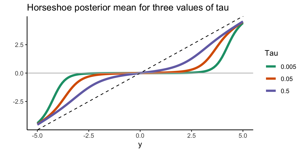

Smaller values of $\tau$ lead to stronger shrinkage behaviour of the horseshoe. Observations that are in absolute value at most equal to $\sqrt{2\sigma^2\log(1/\tau)}$ are shrunk to values close to zero (Van der Pas et al (2014)). For larger observed values, the horseshoe posterior mean will tend to the identity (that is, barely any shrinkage, the estimate will be very close to the observed value). The optimal value of $\tau$ is the proportion of true signals. This value is typically not known in practice but can be estimated, as described further in the next sections.

12.18 The normal means problem

The normal means model is: \[Y_i = \beta_i + \varepsilon_i, \quad i = 1, \ldots, n,\] with $\varepsilon_i$ i.i.d. $\mathcal{N}(0, \sigma^2)$.

First, we will be computing the posterior mean only, with known variance $\sigma^2$ The function HS.post.mean computes the posterior mean of $(\beta_1, \ldots, \beta_n)$. It does not require MCMC and is suitable when only an estimate of the vector $(\beta_1, \ldots, \beta_n)$ is desired. In case uncertainty quantification or variable selection is also of interest, or no good value for $\sigma^2$ is available, please see below for the function HS.normal.means.

The function HS.post.mean requires the observed outcomes, a value for $\tau$ and a value for $\sigma$. Ideally, $\tau$ should be equal to the proportion of nonzero $\beta_i$’s. Typically, this proportion is unknown, in which case it is recommended to use the function HS.MMLE to find the marginal maximum likelihood estimator for $\tau$.

As an example, we generate 50 data points, the first 10 of which are coming from true signals. The first 10 $\beta_i$’s are equal to five and the remaining $\beta_i$’s are equal to zero. Let’s first plot the true parameters (black) and observations (blue).

df <- data.frame(index = 1:50,
                 truth <- c(rep(5, 10), rep(0, 40)),
                 y <- truth + rnorm(50) #observations
                 )

ggplot(data = df, aes(x = index, y = truth)) + 
  geom_point(size = 2) + 
  geom_point(aes(x = index, y = y), size = 2, col = "blue") +
  theme_classic() + ylab("") +
  ggtitle("Black = truth, Blue = observations")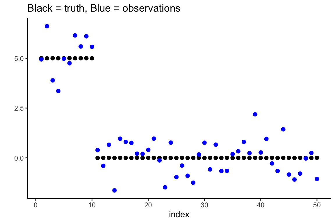

We estimate $\tau$ using the MMLE, using the known variance.

(tau.est <- HS.MMLE(df$y, Sigma2 = 1))

 0.75

We then use this estimate of $\tau$ to find the posterior mean, and add it to the plot in red.

post.mean <- HS.post.mean(df$y, tau.est, 1)
df$post.mean <- post.mean

ggplot(data = df, aes(x = index, y = truth)) + 
  geom_point(size = 2) + 
  geom_point(aes(x = index, y = y), size = 2, col = "blue") +
  theme_classic() + ylab("") +
  geom_point(aes(x = index, y = post.mean), size = 2, col = "red") +
  ggtitle("Black = truth, Blue = observations, Red = estimates")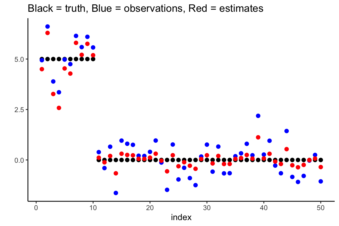

If the posterior variance is of interest, the function HS.post.var can be used. It takes the same arguments as HS.post.mean.

12.18.1 Posterior mean, credible intervals and variable selection, possibly unknown $\sigma^2$

The function HS.normal.means is the main function to use for the normal means problem. It uses MCMC and results in an object that contains all MCMC samples as well as the posterior mean for all parameters ($\beta_i$’s, $\tau$, $\sigma$), the posterior median for the $\beta_i$’s, and credible intervals for the $\beta_i$’s.

The key choices to make are:

How to handle $\tau$. The recommended option is “truncatedCauchy” (a half-Cauchy prior truncated to $[1/n, 1]$). See the manual for other options.
How to handle $\sigma$. The recommended option is “Jeffreys” (Jeffrey’s prior). See the manual for other options.

Other options that can be set by the user are the level of the credible intervals (default is 95%), and the number of MCMC samples (default is 1000 burn-in samples and then 5000 more).

Let’s continue the example from the previous section. We first create a ‘horseshoe object’.

hs.object <- HS.normal.means(df$y, method.tau = "truncatedCauchy", method.sigma = "Jeffreys")

We extract the posterior mean of the $\beta_i$’s and plot them in red.

df$post.mean.full <- hs.object$BetaHat

ggplot(data = df, aes(x = index, y = truth)) + 
  geom_point(size = 2) + 
  geom_point(aes(x = index, y = y), size = 2, col = "blue") +
  theme_classic() + ylab("") +
  geom_point(aes(x = index, y = post.mean.full), size = 2, col = "red") +
  ggtitle("Black = truth, Blue = observations, Red = estimates")

We plot the marginal credible intervals (and remove the observations from the plot for clarity).

df$lower.CI <- hs.object$LeftCI
df$upper.CI <- hs.object$RightCI

ggplot(data = df, aes(x = index, y = truth)) + 
  geom_point(size = 2) + 
  theme_classic() + ylab("") +
  geom_point(aes(x = index, y = post.mean.full), size = 2, col = "red") +
  geom_errorbar(aes(ymin = lower.CI, ymax = upper.CI), width = .1, col = "red") +
  ggtitle("Black = truth, Red = estimates with 95% credible intervals")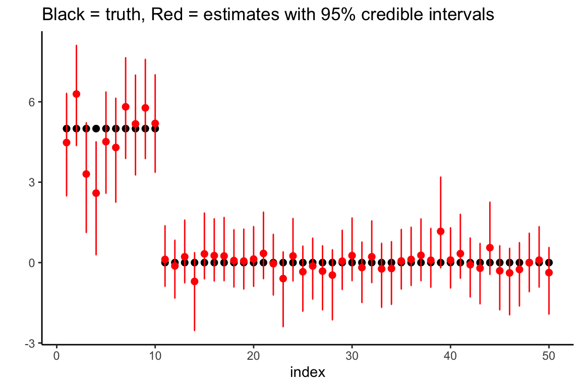

Finally, we perform variable selection using HS.var.select. In the normal means problem, we can use two decision rules. We will illustrate them both. The first method checks whether zero is contained in the credible interval, as studied by Van der Pas et al (2017).

df$selected.CI <- HS.var.select(hs.object, df$y, method = "intervals")

The result is a vector of zeroes and ones, with the ones indicating that the observations is suspected to correspond to an actual signal. We now plot the results, coloring the estimates/intervals blue if a signal is detected and red otherwise.

ggplot(data = df, aes(x = index, y = truth)) + 
  geom_point(size = 2) +
  theme_classic() + ylab("") +
  geom_point(aes(x = index, y = post.mean.full, col = factor(selected.CI)), 
             size = 2) +
  geom_errorbar(aes(ymin = lower.CI, ymax = upper.CI, col = factor(selected.CI)),
                width = .1) +
  theme(legend.position="none") +
  ggtitle("Black = truth, Blue = selected as signal, Red = selected as noise")

The other variable selection method is the thresholding method of Carvalho et al (2010). The posterior mean can be written as $c_iy_i$ where $y_i$ is the observation and $c_i$ some number between 0 and 1. A variable is selected if $c_i \geq c$ for some user-selected threshold $c$ (default is $c = 0.5$). In the example:

df$selected.thres <- HS.var.select(hs.object, df$y, method = "threshold")


ggplot(data = df, aes(x = index, y = truth)) + 
  geom_point(size = 2) +
  theme_classic() + ylab("") +
  geom_point(aes(x = index, y = post.mean.full, col = factor(selected.thres)), 
             size = 2) +
  geom_errorbar(aes(ymin = lower.CI, ymax = upper.CI, col = factor(selected.thres)),
                width = .1) +
  theme(legend.position="none") +
  ggtitle("Black = truth, Blue = selected as signal, Red = selected as noise")

12 Theory of AI

12.1 Choice of loss, penalty and regularisation

12.1.1 Loss

12.1.2 Penalty and Regularisation

12.2 Normal Means Problem

12.2.1 James-Stein Estimator

12.3 \(\ell_2\) Shrinkage

12.3.1 Sparse \(r\)-spike problem

12.3.2 Efron Example

12.4 \(\ell_1\) Sparsity

12.5 \(\ell_0\) Subset Selection

12.6 James-Stein Estimator

12.7 R-spike Problem

12.8 \(\ell_2\) Shrinkage

12.9 \(\ell_1\) Sparsity

12.10 \(\ell_0\) Subset Selection

12.11 Bayesain Model Selection via Regularisation

12.12 Shrinkage (\(\ell_2\) Norm)

12.13 Sparsity (\(\ell_1\) Norm)

12.14 LASSO

12.15 Subset Selection (\(\ell_0\) Norm)

12.16 Bridge (\(\ell_{\alpha}\))

12.16.1 Spike-and-Slab Prior

12.17 Horseshoe Prior

12.18 The normal means problem

12.18.1 Posterior mean, credible intervals and variable selection, possibly unknown \(\sigma^2\)