23 Quantile Neural Networks
GBC Let \((X,Y) \sim P_{X,Y}\) be input-output pairs and \(P_{X,Y}\) a joint measure from which we can simulate a training dataset \((X_i, Y_i)_{i=1}^N \sim P_{X,Y}\). Standard prediction techniques for the conditional posterior mean \(\hat{X}(Y) = E(X|Y) = f(Y)\) of the input given the output. To do this, consider the multivariate non-parametric regression \(X = f(Y) + \epsilon\) and provide methods for estimating the conditional mean. Typically estimators, \(\hat{f}\), include KNN and Kernel methods. Recently, deep learners have been proposed and the theoretical properties of superpositions of affine functions (a.k.a. ridge functions) have been provided (see Montanni and Yang, Schmidt-Hieber, Polson and Rockova).
Generative methods take this approach one step further. Let \(Z \sim P_Z\) be a base measure for a latent variable, \(Z\), typically a standard multivariate normal or vector of uniforms. The goal of generative methods is to characterize the posterior measure \(P_{X|Y}\) from the training data \((X_i, Y_i)_{i=1}^N \sim P_{X,Y}\) where \(N\) is chosen to be suitably large. A deep learner is used to estimate \(\hat{f}\) via the non-parametric regression \(X = f(Y, Z)\). In the case where \(Z\) is uniform, this amounts to inverse cdf sampling, namely \(X = F_{X|Y}^{-1}(U)\).
In general, we characterize the posterior map for any output \(Y\). Simply evaluate the network at any \(Y\) via the transport map \[ X = H(S(Y), \psi(Z)) \] from a new base draw, \(Z\). Here \(\psi\) denotes the cosine embedding so that the architecture for the latent variable corresponds to a Fourier approximation with rates of convergence given by \(O(N^{-\frac{1}{2}})\), see Barron (1993). The deep learner is estimated via a quantile NN from the triples \((X_i, Y_i, Z_i)_{i=1}^N \sim P_{X,Y} \times P_Z\). The ensuing estimator \(\hat{H}_N\) can be thought of as a transport map from the base distribution to the posterior as required.
Specifically, the idea of generative methods is straightforward. Let \(y\) denote data and \(\theta\) a vector of parameters including any hidden states (a.k.a. latent variables) \(z\). First, we generate a “look-up” table of “fake” data \(\{y^{(i)}, \theta^{(i)}\}_{i=1}^N\). By simulating a training dataset of outputs and parameters allows us to use deep learning to solve for the inverse map via a supervised learning problem. Generative methods have the advantage of being likelihood-free. For example, our model might be specified by a forward map \(y^{(i)} = f(\theta^{(i)})\) rather than a traditional random draw from a likelihood function \(y^{(i)} \sim p(y^{(i)}|\theta^{(i)})\).
Generative methods have a number of advantages. First, they are density free. Hence they can be applied in a variety of contexts such as computer simulation, economics where traditional methods are computationally harder. Secondly, they naturally extend to decision problems. Third, they exploit the use of deep neural networks such as Quantile NNs. Hence they naturally provide good forecasting tools.
Posterior uncertainty is solved via the inverse non-parametric regression problem where we predict \(\theta^{(i)}\) from \(y^{(i)}\) and \(\tau^{(i)}\) which is an independent base distribution, \(p(\tau)\). The base distribution is typically uniform or a very large dimensional Gaussian vector. Then we need to train a deep neural network, \(H\), on \[ \theta^{(i)} = H(S(y^{(i)}), \tau^{(i)}). \] Here \(S(y)\) is a statistic to perform dimension reduction with respect to the signal distribution. Specifying \(H\) is the key to the efficiency of the approach. Polson, Ruggeri, and Sokolov (2024) propose the use of quantile neural networks implemented with ReLU activation functions.
23.1 MEU
To extend our generative method to MEU problems, we assume that the utility function \(U\) is given. Then we simply draw additional associated utilities \(U^{(i)}_d \defeq U(d,\theta^{(i)})\) for a given decision \(d\) and \(\theta^{(i)}\) draw from above. Then we append the utilities to our training dataset including the baseline distribution \(\tau^{(i)}\) to yield a new training dataset \[ \{U_d^{(i)}, y^{(i)}, \theta^{(i)}, \tau^{(i)}\}_{i=1}^N. \] Now we construct a non-parametric estimator of the form \[ U_d^{(i)} = H(S(y^{(i)}), \theta^{(i)}, \tau^{(i)}, d), \] Given that the posterior quantiles of the distributional utility, denoted by \(F^{-1}_{U|d,y}(\tau)\) are represented as a quantile neural network, we then use a key identity which shows how to represent any expectation as a marginal over quantiles, namely \[ E_{\theta|y}[U(d, \theta)] = \int_0^1 F^{-1}_{U|d,y}(\tau) d\tau \] The optimal decision function simply maximizes the expected utility \[ d^\star(y) \defeq \arg \max_d E_{\theta|y}[U(d, \theta)] \]
To fix notation and to allow for deterministic updates (a.k.a. measures rather than probabilities). Let \(\mathcal{Y}\) denote a locally compact metric space of signals, denoted by \(y\), and \(\mathcal{B}(\mathcal{Y})\) the Borel \(\sigma\)-algebra of \(\mathcal{Y}\). Let \(\lambda\) be a measure on the measurable space of signals \((\mathcal{Y}, \mathcal{B}(\mathcal{Y}))\). Let \(P(dy|\theta)\) denote the conditional distribution of signals given the parameters. Let \(\Theta\) denote a locally compact metric space of admissible parameters (a.k.a. hidden states and latent variables \(z \in \mathcal{Z}\)) and \(\mathcal{B}(\Theta)\) the Borel \(\sigma\)-algebra of \(\Theta\). Let \(\mu\) be a measure on the measurable space of parameters \((\Theta, \mathcal{B}(\Theta))\). Let \(\Pi(d\theta|y)\) denote the conditional distribution of the parameters given the observed signal \(y\) (a.k.a., the posterior distribution). In many cases, \(\Pi\) is absolutely continuous with density \(\pi\) such that \[ \Pi(d\theta|y) = \pi(\theta|y) \mu(d\theta). \] Moreover, we will write \(\Pi(d\theta) = \pi(\theta) \mu(d\theta)\) for prior density \(\pi\) when available. In the case of likelihood-free models, the output is simply specified by a map (a.k.a. forward equation) \[ y = f(\theta) \] When a likelihood \(p(y|\theta)\) is available w.r.t. the measure \(\lambda\), we write \[ P(dy|\theta) = p(y|\theta) \lambda(dy). \] There are a number of advantages of such an approach, primarily the fact that they are density free. They use simulation methods and deep neural networks to invert the prior to posterior map. We build on this framework and show how to incorporate utilities into the generative procedure.
Noise Outsourcing Theorem If \((Y, \Theta)\) are random variables in a Borel space \((\mathcal{Y}, \Theta)\) then there exists an r.v. \(\tau \sim U(0,1)\) which is independent of \(Y\) and a function \(H: [0,1] \times \mathcal{Y} \rightarrow \Theta\) such that \[ (Y, \Theta) \stackrel{a.s.}{=} (Y, H(Y, \tau)) \] Hence the existence of \(H\) follows from the noise outsourcing theorem Kallenberg (1997). Moreover, if there is a statistic \(S(Y)\) with \(Y \independent \Theta | S(Y)\), then \[ \Theta|Y \stackrel{a.s.}{=} H(S(Y), \tau). \] The role of \(S(Y)\) is equivalent to the ABC literature. It performs dimension reduction in \(n\), the dimensionality of the signal. Our approach then is to use deep neural network first to calculate the inverse probability map (a.k.a posterior) \(\theta \stackrel{D}{=} F^{-1}_{\theta|y}(\bm{\tau})\) where \(\bm{\tau}\) is a vector of uniforms. In the multi-parameter case, we use an RNN or autoregressive structure where we model a vector via a sequence \((F^{-1}_{\theta_1}(\tau_1), F^{-1}_{\theta_2|\theta_1}(\tau_2), \ldots)\). A remarkable result due to Brillinger (2012) shows that we can learn \(S\) independent of \(H\) simply via OLS.
As a default choice of network architecture, we will use a ReLU network for the posterior quantile map. The first layer of the network is given by the utility function and hence this is what makes the method different from learning the posterior and then directly using naive Monte Carlo to estimate expected utility. This would be inefficient as quite often the utility function places high weight on region of low-posterior probability representing tail risk.
23.2 Bayes Rule for Quantiles
Parzen (2004) shows that quantile methods are direct alternatives to density computations. Specifically, given \(F_{\theta|y} (u)\), a non-decreasing and continuous from right function, we define
\[Q_{\theta| y} (u) \defeq F^{-1}_{\theta|y} ( u ) = \inf \left ( \theta : F_{\theta|y} (\theta) \geq u \right )\]
which is non-decreasing, continuous from left.
Parzen (2004) shows the important probabilistic property of quantiles
\[\theta \stackrel{P}{=} Q_\theta ( F_\theta (\theta ) )\]
Hence, we can increase the efficiency by ordering the samples of \(\theta\) and the baseline distribution and use monotonicity of the inverse CDF map.
Let \(g(y)\) be non-decreasing and continuous from left with \(g^{-1} (z ) = \sup \left ( y : g(y ) \leq z \right )\). Then, the transformed quantile has a compositional nature, namely
\[Q_{ g(Y) } ( u ) = g ( Q (u ))\]
Hence, quantiles act as superposition (a.k.a. deep Learner).
This is best illustrated in the Bayes learning model. We have the following result updating prior to posterior quantiles known as the conditional quantile representation
\[Q_{ \theta | Y=y } ( u ) = Q_\theta ( s ) \; \; {\rm where} \; \; s = Q_{ F(\theta) | Y=y } ( u)\]
To compute \(s\), by definition
\[u = F_{ F(\theta ) | Y=y} ( s ) = P( F (\theta ) \leq s | Y=y ) = P( \theta \leq Q_\theta (s ) | Y=y ) = F_{ \theta | Y=y } ( Q_\theta ( s ) )\]
23.2.1 Maximum Expected Utility
Decision problems are characterized by a utility function \(U( \theta , d )\) defined over parameters, \(\theta\), and decisions, \(d \in \mathcal{D}\). We will find it useful to define the family of utility random variables indexed by decisions defined by
\[U_d \defeq U( \theta , d ) \; \; {\rm where} \; \; \theta \sim \Pi ( d \theta )\]
Optimal Bayesian decisions are then defined by the solution to the prior expected utility
\[U(d) = E_{\theta}(U(d,\theta)) = \int U(d,\theta)p(\theta)d\theta\]
\[d^\star = {\rm arg} \max_d U(d)\]
When information in the form of signals \(y\) is available, we need to calculate the posterior distribution \(p( \theta | y ) = f(y | \theta ) p( \theta )/ p(y)\). Then we have to solve for the optimal a posterior decision rule \(d^\star (y)\) defined by
\[d^\star(y) = {\rm arg} \max_d \; \int U( \theta , d ) p( \theta | y ) d \theta\]
where expectations are now taken w.r.t. \(p( \theta | y)\) the posterior distribution.
23.3 Normal-Normal Bayes Learning: Wang Distortion
For the purpose of illustration, we consider the normal-normal learning model. We will develop the necessary quantile theory to show how to calculate posteriors and expected utility without resorting to densities. Also, we show a relationship with Wang’s risk distortion measure as the deep learning that needs to be learned.
Specifically, we observe the data \(y = ( y_1,\ldots,y_n)\) from the following model
\[y_1 , \ldots , y_n \mid \theta \sim N(\theta, \sigma^2)\]
\[\theta \sim N(\mu,\alpha^2)\]
Hence, the summary (sufficient) statistic is \(S(y) = \bar y = \frac{1}{n} \sum_{i=1}^n y_i\).
Given observed samples \(y = (y_1,\ldots,y_n)\), the posterior is then \(\theta \mid y \sim N(\mu_*, \sigma_*^2)\) with
\[\mu_* = (\sigma^2 \mu + \alpha^2s) / t, \quad \sigma^2_* = \alpha^2 \sigma^2 / t\]
where
\[t = \sigma^2 + n\alpha^2 \; \; {\rm and} \; \; s(y) = \sum_{i=1}^{n}y_i\]
The posterior and prior CDFs are then related via the
\[1-\Phi(\theta, \mu_*,\sigma_*) = g(1 - \Phi(\theta, \mu, \alpha^2))\]
where \(\Phi\) is the normal distribution function. Here the Wang distortion function defined by
\[g(p) = \Phi\left(\lambda_1 \Phi^{-1}(p) + \lambda\right)\]
where
\[\lambda_1 = \dfrac{\alpha}{\sigma_*} \; \; {\rm and} \; \; \lambda = \alpha\lambda_1(s-n\mu)/t\]
The proof is relatively simple and is as follows
\[\begin{align*} g(1 - \Phi(\theta, \mu, \alpha^2)) & = g(\Phi(-\theta, \mu, \alpha^2)) = g\left(\Phi\left(-\dfrac{\theta - \mu}{\alpha}\right)\right)\\ & = \Phi\left(\lambda_1 \left(-\dfrac{\theta - \mu}{\alpha}\right) + \lambda\right) = 1 - \Phi\left(\dfrac{\theta - (\mu+ \alpha\lambda/\lambda_1)}{\alpha/\lambda_1}\right) \end{align*}\]
Thus, the corresponding posterior updated parameters are
\[\sigma_* = \alpha/\lambda_1, \quad \lambda_1 = \dfrac{\alpha}{\sigma_*}\]
and
\[\mu_* = \mu+ \alpha\lambda/\lambda_1, \quad \lambda = \dfrac{\lambda_1(\mu_* - \mu)}{\alpha} = \alpha\lambda_1(s-n\mu)/t\]
We now provide an empirical example.
23.3.1 Numerical Example
Consider the normal-normal model with Prior \(\theta \sim N(0,5)\) and likelihood \(y \sim N(3,10)\). We generate \(n=100\) samples from the likelihood and calculate the posterior distribution.
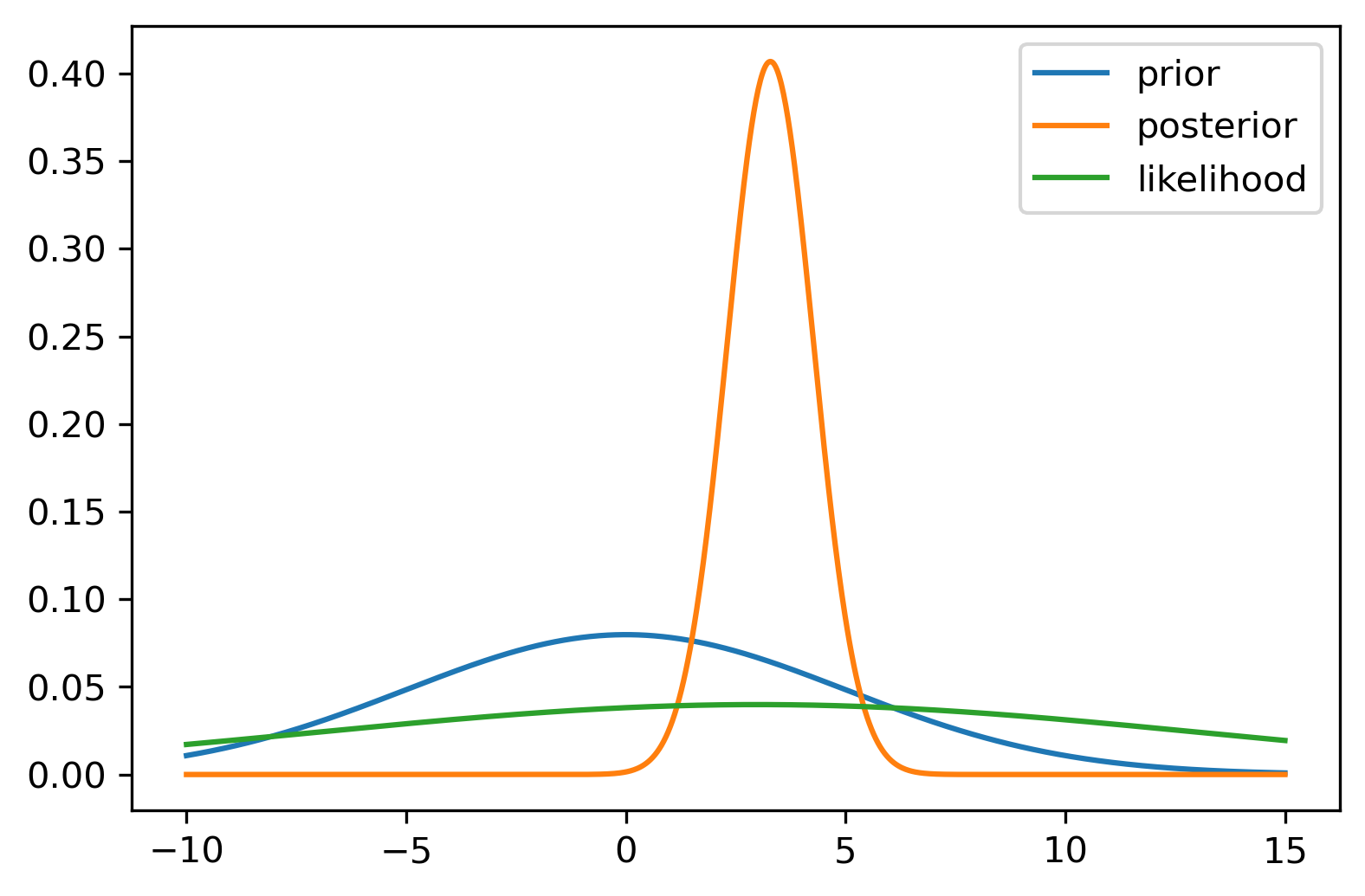
The posterior distribution calculated from the sample is then \(\theta \mid y \sim N(3.28, 0.98)\).
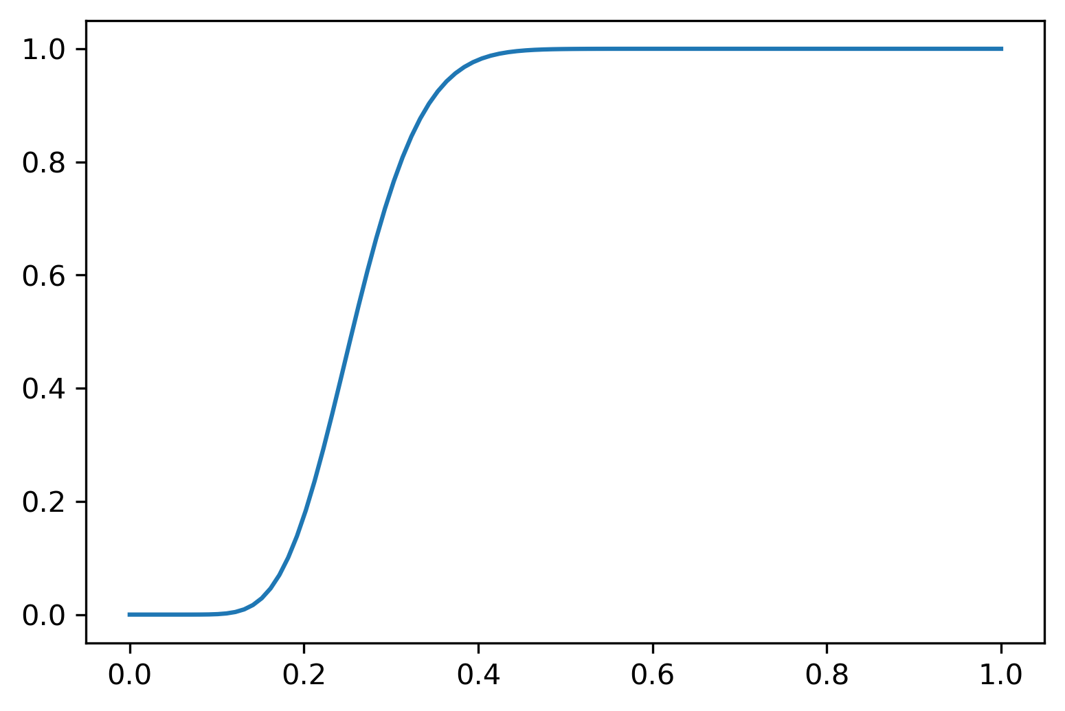
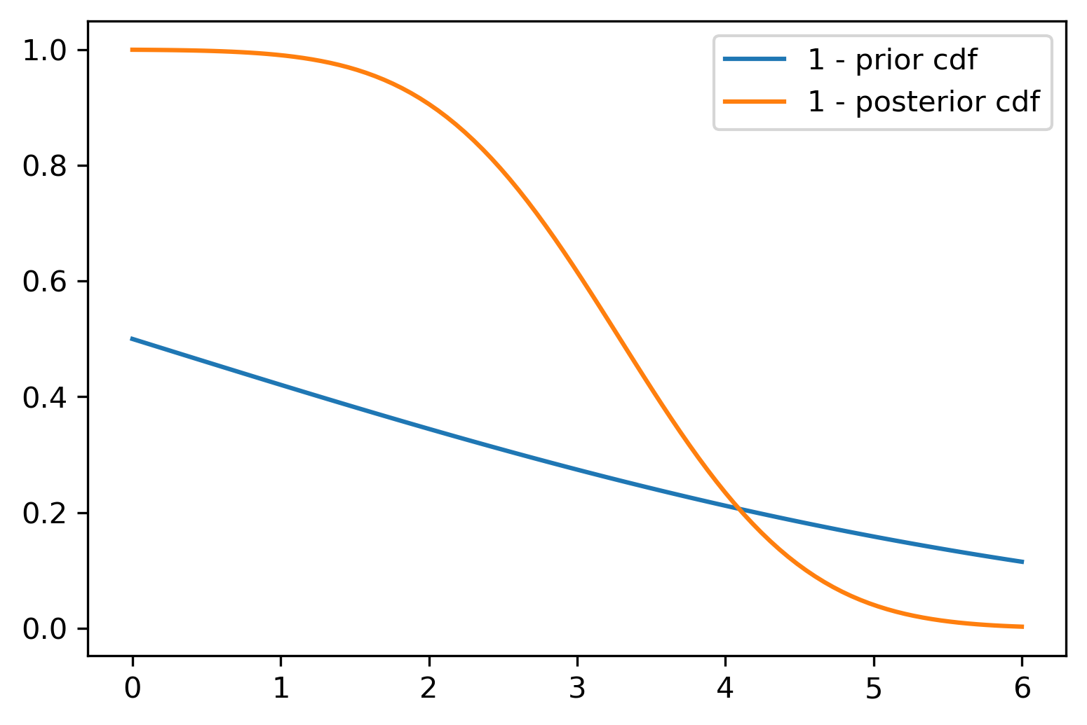
Figure 23.2 shows the Wang distortion function for the normal-normal model. The left panel shows the model for the simulated data, while the middle panel shows the distortion function, the right panel shows the 1 - \(\Phi\) for the prior and posterior of the normal-normal model.
23.4 Portfolio Learning
Consider power utility and log-normal returns (without leverage). For \(\omega \in (0,1)\)
\[U(W) = -e^{-\gamma W}, ~ W\mid \omega \sim \mathcal{N}( (1-\omega) r_f + \omega R,\sigma^2)\]
Let \(W = (1-\omega)r_f + \omega R\), with \(R \sim N(\mu,\sigma^2)\), Here, \(U^{-1}\) exists and \(r_f\) is the risk-free rate, \(\mu\) is the mean return and \(\tau^2\) is the variance of the return. Then the expected utility is
\[U(\omega) = E(-e^{\gamma W}) = \exp\left\{\gamma E(W) + \frac{1}{2}\omega^2Var(W)\right\}\]
We have closed-form utility in this case, since it is the moment-generating function of the log-normal. Within the Gen-AI framework, it is easy to add learning or uncertainty on top of \(\sigma^2\) and have a joint posterior distribution \(p(\mu, \sigma^2 \mid R)\).
Thus, the closed form solution is
\[U(\omega) = \exp\left\{\gamma \left\{(1-\omega)r_f + \omega\mu\right\}\right\} \exp \left \{ \dfrac{1}{2}\gamma^2\omega^2\sigma^2 \right \}\]
The optimal Kelly-Brieman-Thorpe-Merton rule is given by
\[\omega^* = (\mu - r_f)/(\sigma^2\gamma)\]
Now we reorder the integral in terms of quantiles of the utility function. We assume utility is the random variable and re-order the sum as the expected value of \(U\)
\[E(U(W)) = \int_{0}^{1}F_{U(W)}^{-1}(\tau)d\tau\]
Hence, if we can approximate the inverse of the CDF of \(U(W)\) with a quantile NN, we can approximate the expected utility and optimize over \(\omega\).
The stochastic utility is modeled with a deep neural network, and we write
23.5 Bayes Rule for Quantiles
Parzen (2004) shows that quantile methods are direct alternatives to density computations. Specifically, given \(F_{\theta|y} (u)\), a non-decreasing and continuous from right function, we define
\[Q_{\theta| y} (u) \defeq F^{-1}_{\theta|y} ( u ) = \inf \left ( \theta : F_{\theta|y} (\theta) \geq u \right )\]
which is non-decreasing, continuous from left. Parzen (2004) shows the important probabilistic property of quantiles \[ \theta \stackrel{P}{=} Q_\theta ( F_\theta (\theta ) ) \] Hence, we can increase the efficiency by ordering the samples of \(\theta\) and the baseline distribution and use monotonicity of the inverse CDF map.
Let $ g(y)$ be non-decreasing and continuous from left with $g^{-1} (z ) = ( y : g(y ) z ) \(. Then, the transformed quantile has a compositional nature, namely\)$ Q_{ g(Y) } ( u ) = g ( Q (u )) $$ Hence, quantiles act as superposition (a.k.a. deep Learner).
This is best illustrated in the Bayes learning model. We have the following result updating prior to posterior quantiles known as the conditional quantile representation \[ Q_{ \theta | Y=y } ( u ) = Q_\theta ( s ) \; \; {\rm where} \; \; s = Q_{ F(\theta) | Y=y } ( u) \] To compute \(s\), by definition \[ u = F_{ F(\theta ) | Y=y} ( s ) = P( F (\theta ) \leq s | Y=y ) = P( \theta \leq Q_\theta (s ) | Y=y ) = F_{ \theta | Y=y } ( Q_\theta ( s ) ) \]
Decision problems are characterized by a utility function $ U( , d ) $ defined over parameters, $ $, and decisions, $ d \(. We will find it useful to define the family of utility random variables indexed by decisions defined by\)$ U_d U( , d ) ; ; {} ; ; ( d ) \[ Optimal Bayesian decisions \cite{degroot2005optimal} are then defined by the solution to the prior expected utility \[ U(d) = E_{\theta}(U(d,\theta)) = \int U(d,\theta)p(\theta)d\theta, \] \] d^= {} _d U(d) \[ When information in the form of signals $y$ is available, we need to calculate the posterior distribution $p( \theta | y ) = f(y | \theta ) p( \theta )/ p(y)$. Then we have to solve for the optimal \emph{a posterior} decision rule $ d^\star (y) $ defined by \] d^(y) = {} _d ; U( , d ) p( | y ) d $$ where expectations are now taken w.r.t. $ p( | y) $ the posterior distribution.
23.6 Normal-Normal Bayes Learning: Wang Distortion
For the purpose of illustration, we consider the normal-normal learning model. We will develop the necessary quantile theory to show how to calculate posteriors and expected utility without resorting to densities. Also, we show a relationship with Wang’s risk distortion measure as the deep learning that needs to be learned.
Specifically, we observe the data \(y = (y_1,\ldots,y_n)\) from the following model
\[y_1 , \ldots , y_n \mid \theta \sim N(\theta, \sigma^2)\] \[\theta \sim N(\mu,\alpha^2)\]
Hence, the summary (sufficient) statistic is \(S(y) = \bar y = \frac{1}{n} \sum_{i=1}^n y_i\).
Given observed samples \(y = (y_1,\ldots,y_n)\), the posterior is then \(\theta \mid y \sim N(\mu_*, \sigma_*^2)\) with
\[\mu_* = (\sigma^2 \mu + \alpha^2s) / t, \quad \sigma^2_* = \alpha^2 \sigma^2 / t\]
where
\[t = \sigma^2 + n\alpha^2 \; \; {\rm and} \; \; s(y) = \sum_{i=1}^{n}y_i\]
The posterior and prior CDFs are then related via the
\[1-\Phi(\theta, \mu_*,\sigma_*) = g(1 - \Phi(\theta, \mu, \alpha^2))\]
where \(\Phi\) is the normal distribution function. Here the Wang distortion function defined by
\[g(p) = \Phi\left(\lambda_1 \Phi^{-1}(p) + \lambda\right)\]
where
\[\lambda_1 = \dfrac{\alpha}{\sigma_*} \; \; {\rm and} \; \; \lambda = \alpha\lambda_1(s-n\mu)/t\]
The proof is relatively simple and is as follows
\[g(1 - \Phi(\theta, \mu, \alpha^2)) = g(\Phi(-\theta, \mu, \alpha^2)) = g\left(\Phi\left(-\dfrac{\theta - \mu}{\alpha}\right)\right)\]
\[= \Phi\left(\lambda_1 \left(-\dfrac{\theta - \mu}{\alpha}\right) + \lambda\right) = 1 - \Phi\left(\dfrac{\theta - (\mu+ \alpha\lambda/\lambda_1)}{\alpha/\lambda_1}\right)\]
Thus, the corresponding posterior updated parameters are
\[\sigma_* = \alpha/\lambda_1, \quad \lambda_1 = \dfrac{\alpha}{\sigma_*}\]
and
\[\mu_* = \mu+ \alpha\lambda/\lambda_1, \quad \lambda = \dfrac{\lambda_1(\mu_* - \mu)}{\alpha} = \alpha\lambda_1(s-n\mu)/t\]
We now provide an empirical example.
23.6.1 Numerical Example
Consider the normal-normal model with Prior \(\theta \sim N(0,5)\) and likelihood \(y \sim N(3,10)\). We generate \(n=100\) samples from the likelihood and calculate the posterior distribution.


The posterior distribution calculated from the sample is then \(\theta \mid y \sim N(3.28, 0.98)\).
Figure 23.2 shows the Wang distortion function for the normal-normal model. The left panel shows the model for the simulated data, while the middle panel shows the distortion function, the right panel shows the 1 - \(\Phi\) for the prior and posterior of the normal-normal model.
23.7 Portfolio Learning
Consider power utility and log-normal returns (without leverage). For \(\omega \in (0,1)\)
\[U(W) = -e^{-\gamma W}, ~ W\mid \omega \sim \mathcal{N}( (1-\omega) r_f + \omega R,\sigma^2)\]
Let \(W = (1-\omega)r_f + \omega R\), with \(R \sim N(\mu,\sigma^2)\), Here, \(U^{-1}\) exists and \(r_f\) is the risk-free rate, \(\mu\) is the mean return and \(\tau^2\) is the variance of the return. Then the expected utility is
\[U(\omega) = E(-e^{\gamma W}) = \exp\left\{\gamma E(W) + \frac{1}{2}\omega^2Var(W)\right\}\]
We have closed-form utility in this case, since it is the moment-generating function of the log-normal. Within the Gen-AI framework, it is easy to add learning or uncertainty on top of \(\sigma^2\) and have a joint posterior distribution \(p(\mu, \sigma^2 \mid R)\).
Thus, the closed form solution is
\[U(\omega) = \exp\left\{\gamma \left\{(1-\omega)r_f + \omega\mu\right\}\right\} \exp \left \{ \dfrac{1}{2}\gamma^2\omega^2\sigma^2 \right \}\]
The optimal Kelly-Brieman-Thorpe-Merton rule is given by
\[\omega^* = (\mu - r_f)/(\sigma^2\gamma)\]
Now we reorder the integral in terms of quantiles of the utility function. We assume utility is the random variable and re-order the sum as the expected value of \(U\)
\[E(U(W)) = \int_{0}^{1}F_{U(W)}^{-1}(\tau)d\tau\]
Hence, if we can approximate the inverse of the CDF of \(U(W)\) with a quantile NN, we can approximate the expected utility and optimize over \(\omega\).
The stochastic utility is modeled with a deep neural network, and we write
\[Z = U(W) \approx F, ~ W = U^{-1}(F)\]
We can do optimization by doing the grid for \(\omega\).
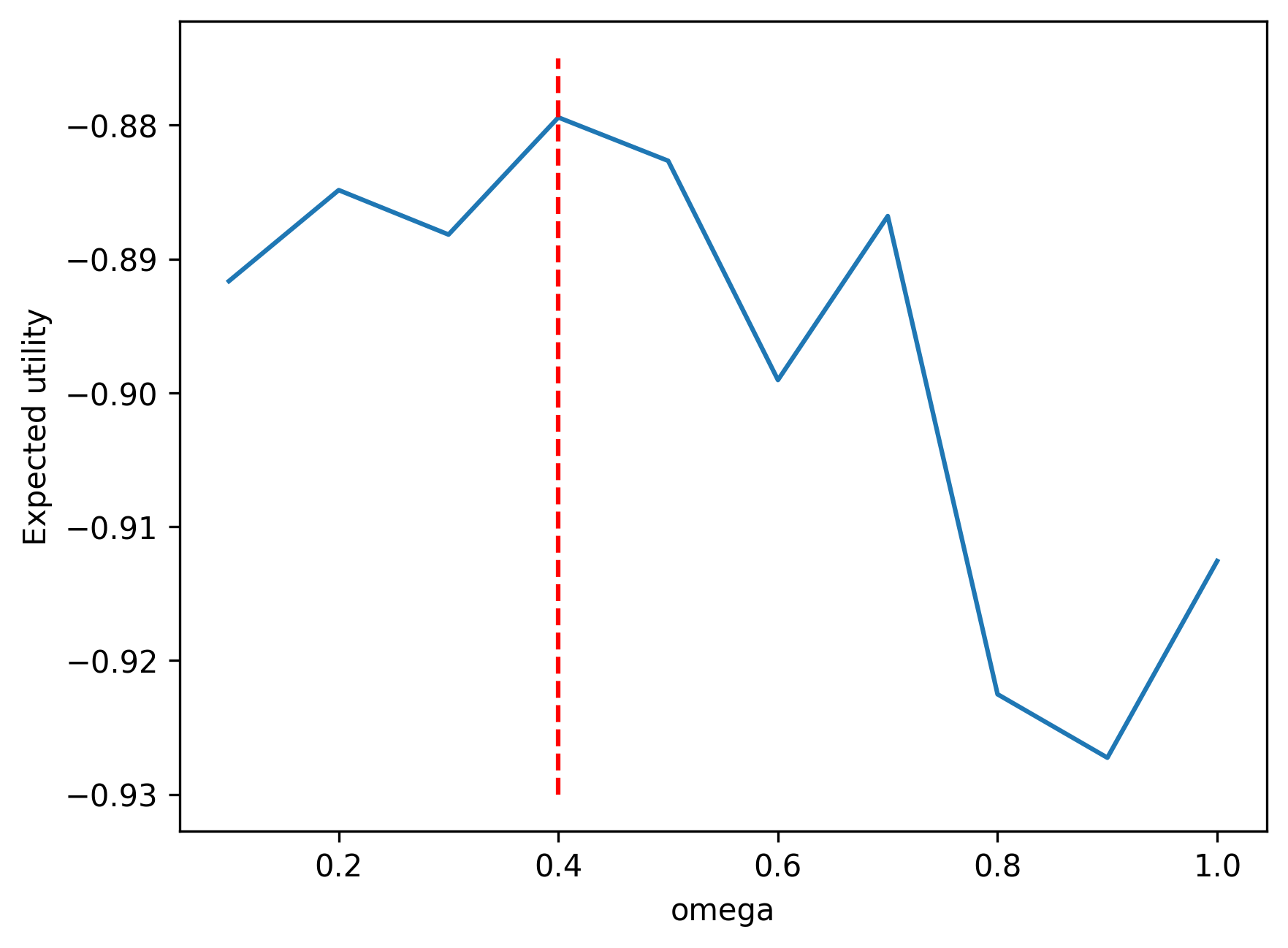
23.7.1 Empirical Example
Consider \(\omega \in (0,1)\), \(r_f = 0.05\), \(\mu=0.1\), \(\sigma=0.25\), \(\gamma = 2\). We have the closed-form fractional Kelly criterion solution
\[\omega^* = \frac{1}{\gamma} \frac{ \mu - r_f}{ \sigma^2} = \frac{1}{2} \frac{ 0.1 - 0.05 }{ 0.25^2 } = 0.40\]
We can simulate the expected utility and compare with the closed-form solution.
Add code.
23.8 Learning Quantiles
The 1-Wasserstein distance is the \(\ell_1\) metric on the inverse distribution function. It is also known as earth mover’s distance and can be calculated using order statistics (Levina and Bickel 2001). For quantile functions \(F^{-1}_U\) and \(F^{-1}_V\) the 1-Wasserstein distance is given by
\[ W_1(F^{-1}_U, F^{-1}_V) = \int_0^1 |F^{-1}_U(\tau) - F^{-1}_V(\tau)| d\tau \]
It can be shown that Wasserstein GAN networks outperform vanilla GAN due to the improved quantile metric. \(q = F^{-1}_U(\tau)\) minimizes the expected quantile loss
\[ E_U[\rho_{\tau}(u-q)] \]
Quantile regression can be shown to minimize the 1-Wasserstein metric. A related loss is the quantile divergence,
\[ q(U,V) = \int_0^1 \int_{F^{-1}_U(q)}^{F^{-1}_V(q)} (F_U(\tau)-q) dq d\tau \]
The quantile regression likelihood function is an asymmetric function that penalizes overestimation errors with weight \(\tau\) and underestimation errors with weight \(1-\tau\). For a given input-output pair \((x, y)\), and the quantile function \(f(x, \theta)\), parametrized by \(\theta\), the quantile loss is \(\rho_{\tau}(u) = u(\tau - I(u < 0))\), where \(u = y - f(x)\). From the implementation point of view, a more convenient form of this function is
\[ \rho_{\tau}(u) = \max(u\tau, u(\tau-1)) \]
Given a training data \(\{x_i, y_i\}_{i=1}^N\), and given quantile \(\tau\), the loss is
\[ L_{\tau}(\theta) = \sum_{i=1}^N \rho_{\tau}(y_i - f(\tau, x_i, \theta)) \]
Further, we empirically found that adding a mean-squared loss to this objective function improves the predictive power of the model, thus the loss function we use is
\[ \alpha L_{\tau}(\theta) + \frac{1}{N} \sum_{i=1}^N (y_i - f(x_i, \theta))^2 \]
One approach to learn the quantile function is to use a set of quantiles \(0 < \tau_1 < \tau_2 < \ldots < \tau_K < 1\) and then learn \(K\) quantile functions simultaneously by minimizing
\[ L(\theta, \tau_1, \ldots, \tau_K) = \frac{1}{N K} \sum_{i=1}^N \sum_{k=1}^K \rho_{\tau_k}(y_i - f_{\tau_k}(x_i, \theta_k)) \]
The corresponding optimization problem of minimizing \(L(\theta)\) can be augmented by adding a non-crossing constraint
\[ f_{\tau_i}(x, \theta_i) < f_{\tau_j}(x, \theta_j), \quad \forall x, \; i < j \]
The non-crossing constraint has been considered by several authors, including (Chernozhukov, Fernández-Val, and Galichon 2010; Cannon 2018).
23.8.1 Cosine Embedding for \(\tau\)
To learn an inverse CDF (quantile function) \(F^{-1}(\tau, y) = f_\theta(\tau, y)\) we will use a kernel embedding trick and augment the predictor space. We then represent the quantile function as a function of superposition for two other functions:
\[ F^{-1}(\tau, y) = f_\theta(\tau, y) = g(\psi(y) \circ \phi(\tau)) \]
where \(\circ\) is the element-wise multiplication operator. Both functions \(g\) and \(\psi\) are feed-forward neural networks. \(\phi\) is a cosine embedding. To avoid over-fitting, we use a sufficiently large training dataset, see (Dabney et al. 2018) in a reinforcement learning context.
Let \(g\) and \(\psi\) be feed-forward neural networks and \(\phi\) a cosine embedding given by
\[ \phi_j(\tau) = \mathrm{ReLU}\left(\sum_{i=0}^{n-1} \cos(\pi i \tau) w_{ij} + b_j\right) \]
We now illustrate our approach with a simple synthetic dataset.
23.9 Synthetic Data
Consider a synthetic data generated from the model
\[ x \sim U(-1, 1) \\ y \sim N(\sin(\pi x)/(\pi x), \exp(1-x)/10) \]
The true quantile function is given by
\[ f_{\tau}(x) = \sin(\pi x)/(\pi x) + \Phi^{-1}(\tau) \sqrt{\exp(1-x)/10} \]

We train two quantile networks, one implicit and one explicit. The explicit network is trained for three fixed quantiles \((0.05, 0.5, 0.95)\). The figure above shows fits by both of the networks; we see no empirical difference between the two.
23.10 Quantiles as Deep Learners
One can show that quantile models are direct alternatives to other Bayes computations. Specifically, given \(F(y)\), a non-decreasing and continuous from right function, we define
\[ Q_{\theta|y}(u) \defeq F^{-1}_{\theta|y}(u) = \inf\{y : F_{\theta|y}(y) \geq u\} \]
which is non-decreasing, continuous from left. Now let \(g(y)\) be a non-decreasing and continuous from left with
\[ g^{-1}(z) = \sup\{y : g(y) \leq z\} \]
Then, the transformed quantile has a compositional nature, namely
\[ Q_{g(Y)}(u) = g(Q(u)) \]
Hence, quantiles act as superposition (a.k.a. deep learner).
This is best illustrated in the Bayes learning model. We have the following result updating prior to posterior quantiles known as the conditional quantile representation:
\[ Q_{\theta | Y=y}(u) = Q_Y(s) \] where \(s = Q_{F(\theta) | Y=y}(u)\)
To compute \(s\) we use
\[ u = F_{F(\theta) | Y=y}(s) = P(F(\theta) \leq s | Y=y) = P(\theta \leq Q_\theta(s) | Y=y) = F_{\theta | Y=y}(Q_\theta(s)) \]
(Parzen 2004) also shows the following probabilistic property of quantiles:
\[ \theta = Q_\theta(F_\theta(\theta)) \]
Hence, we can increase the efficiency by ordering the samples of \(\theta\) and the baseline distribution as the mapping being the inverse CDF is monotonic.
23.10.1 Quantile Reinforcement Learning
(Dabney et al. 2017) use quantile neural networks for decision-making and apply quantile neural networks to the problem of reinforcement learning. Specifically, they rely on the fact that expectations are quantile integrals. The key identity in this context is the Lorenz curve:
\[ E(Y) = \int_{-\infty}^{\infty} y dF(y) = \int_0^1 F^{-1}(u) du \]
Then, distributional reinforcement learning algorithm finds
\[ \pi(x) = \arg\max_a E_{Z \sim z(x, a)}(Z) \]
Then a Q-Learning algorithm can be applied, since the quantile projection keeps contraction property of Bellman operator. Similar approaches that rely on the dual Expected Utility were proposed by (Yaari 1987).