SELECT randomized 17,604 adults with overweight or obesity and established cardiovascular disease, without diabetes, to weekly semaglutide 2.4 mg or placebo, at 804 sites in 41 countries, enrolling from 2018 to 2021 (Lincoff et al. 2023). The primary endpoint, a composite of cardiovascular death, nonfatal myocardial infarction and nonfatal stroke, occurred in 569 of 8,803 patients on semaglutide and 701 of 8,801 on placebo: 1,270 events in all, a hazard ratio of 0.80 with a 95 percent confidence interval from 0.72 to 0.90. Mean follow-up was 39.8 months. A result of this kind changes practice, and it was earned honestly: the trial was designed for a hazard ratio of 0.83 with 90 percent power at one-sided 0.025, 1,225 planned events, and one superiority interim analysis at two thirds of them (Ryan et al. 2020). At that interim (831 events) the data monitoring committee recommended continuing (FDA clinical review), so the trial ran to its end.
ImportantRegulatory anchor
Section 505(d) of the Federal Food, Drug, and Cosmetic Act(United States Congress 1962). The statutory standard: a drug is approved on “substantial evidence” of effectiveness, which the Act defines as evidence consisting of adequate and well-controlled investigations. Statute, binding.
21 CFR 314.126(U.S. Food and Drug Administration 2024). The regulation that says what “adequate and well-controlled” means: a clear objective, a valid comparison with a control, measures against bias, and an analysis adequate to assess the effect. Regulation, binding.
ICH E8(R1), General Considerations for Clinical Studies(International Council for Harmonisation 2021) (Step 4, October 2021). Asks that quality be designed in before the study starts (“quality by design”), by identifying what is critical to the decision the trial will support. Final guideline.
ICH E9, Statistical Principles for Clinical Trials(International Council for Harmonisation 1998) (Step 4, 1998). The statistical standard that most protocols still follow: pre-specified analysis, control of type I error, and justification of sample size. Final guideline, with the E9(R1) addendum on estimands (International Council for Harmonisation 2019) (Step 4, November 2019).
FDA draft guidance on Bayesian methodology(U.S. Food and Drug Administration 2026) (January 2026). Draft, not binding. It is the first FDA guidance on Bayesian methods for drugs and biological products (devices have had one since 2010), and it allows a success criterion to be calibrated to type I error, read from the posterior, or based on a decision-theoretic rule or a benefit-risk threshold.
The full map, with status and dates, is in Chapter 3.
The question this book asks is the one the trial raises. Hold the error rate fixed at the level the design promised. When could the answer have been known, and what did waiting cost? Every month before a result is known, half the participants are on placebo, and a drug that works is withheld from them while the trial runs.
Here is the answer in headline form, as a counterfactual reconstruction of ours and not a statement about what the sponsor or the committee did. Suppose the true hazard ratio is 0.80 and the trial can run to at most 1,270 events, and simulate 40,000 such trials (details in Chapter 21). A Bayes rule monitored on the prespecified event grid (every second event), with its posterior threshold calibrated so that the type I error is 2.5 percent, stops at a median of 464 events among the simulated trials that declare efficacy. SELECT’s planned design, with its one interim, stops at a median of 817 events when it succeeds, and a four-look O’Brien-Fleming design at 952. Counting every simulated trial, where noncrossing trials end at each rule’s maximum (1,270 events for the hypothetical rules and 1,225 for SELECT’s planned two-look design), the medians are 486, 817 and 952. The powers are 95, 97 and 98 percent, and the realized type I errors are 2.5, 2.5 and 2.5 percent, so the comparison is between rules held to the same 2.5 percent ceiling. The Bayesian figure is fixed at 2.5 by construction, because the threshold is calibrated on the same simulated null paths; an independent check on fresh paths, with its Monte Carlo uncertainty, is in Chapter 21. An anytime-valid e-value rule, also in the reconstruction, stops at a median of 612 events among successes but acts in only 83 percent of trials, because it is conservative (a realized type I error of 0.6 percent).
Under a modeled accrual (calendar time is a counterfactual, not an observation), a Bayes decision at the conditional median events would fall about 16 months before the four-look design’s and 27 months before the read-out, and about 18,500 modeled placebo patient-years would accrue after that point. The gain is earlier stopping at a calibrated bar, not a lower bar: the same Bayes rule at the conventional 0.975, checked on the same grid, would have a type I error of 11.8 percent.
What waiting cost, in three currencies. Every figure in this paragraph and in Table 1.1 is a modeled counterfactual of ours, computed from the all-trial distribution of simulated stopping points, in which a trial that never crosses is counted at its maximum and so saves nothing. Averaged over all simulated trials the Bayes rule had accrued 44 percent of SELECT’s events when it stopped, so on average 56 percent of the events and of the person time would have come afterwards, and the all-trial median decision falls 2.2 years before the read-out under the accrual model above. The three currencies are the trial cost avoided, the cardiovascular label reached earlier inside a fixed patent life (so that label-driven revenue is brought forward), and the health value of the events and quality-adjusted life years (QALYs) the placebo arm would have been spared.
Table 1.1: What waiting cost in SELECT, in three currencies, all modeled counterfactuals from the all-trial stopping distribution. Dollar figures are not profits and not forecasts.
currency
SELECT, modeled
assumption that carries it
(a) trial cost avoided
$44 million to $237 million
a variable share of cost of 50 to 70 percent, on a total of $157 million, the cardiovascular mean of published pivotal-trial cost estimates (Moore et al. 2018), up to $600 million (a scenario for a larger trial)
(b) label revenue brought forward
$1.8 billion to $4.6 billion of Wegovy revenue, not profit
2024 global sales of DKK 58.2 billion (Novo Nordisk A/S 2025) at an assumed 6.9 DKK per dollar, 10 to 25 percent of sales attributable to the cardiovascular label (an assumption, not a public figure), brought forward by 2.2 years; an upper bound
(c) health value
in the trial about 75 excess placebo-arm primary events averted and 112 to 224 QALYs; outside it, as a bound, about 10,400 events per million patients treated
events uniform in person time, placebo participants switched at the decision, 1.5 to 3 QALYs per event; the bound adds a placebo event rate of 2.4 percent a year, a 20 percent relative reduction and instant uptake over the whole window
These are not savings the sponsor or the committee forgone: they say what the evidence would have permitted at a calibrated bar, and each currency stacks assumptions on the one before, so the trial cost is the firmest and the population bound the loosest. Two cautions apply to all of them. Among trials stopping early for efficacy, naive estimates tend to exaggerate benefit. Skeptical priors may reduce this bias; bias and interval coverage should be evaluated for the specified estimator and stopping rule. And a regulator wants safety follow-up that would continue after an efficacy decision, which recovers only part of the cost saving. The same reconstruction for REWIND crosses in only 49 percent of the simulated trials, so the all-trial median saving there is zero, although the unconditional expected saving can still be positive (Section 21.6); the counterweight below stands. The full accounting, with the REWIND figures stated conditionally, is in Section 21.6.
The counterweight is a trial with a smaller effect. REWIND, the dulaglutide cardiovascular trial, reported a hazard ratio of 0.88 on 1,257 events (Gerstein et al. 2019). Reconstructed in the same way, the four-look O’Brien-Fleming design acts by the end with probability 0.61 and the Bayes rule with probability 0.49, so the scheduled design acts more often there, even though the Bayes rule decides earlier when it decides (median 680 events against 942). The book is about when each of these holds and how to show it by simulation before the trial starts. SELECT returns in Chapter 21 with the full reconstruction.
Drug development usually fails, a pivotal trial is expensive and takes years, and a day of delay at the end is worth more than most trials cost per week. A design that reaches the same legal standard of evidence with fewer patients and less time is therefore not a refinement. It is the main thing a sponsor can still change. This chapter makes that case with published numbers first, and only then turns to the machinery. Every figure quoted here is cited; where a figure is a simulation or a registry search, we say so.
1.2 A ledger before the trial
The decision view of medical evidence is older than the randomized trial, and its first great practitioner was a nurse. Polson and Scott tell the story in AIQ as the beginning of the idea that the numbers a hospital already collects can change what the hospital does (Polson and Scott 2018). Florence Nightingale worked at the British army’s Barrack Hospital at Scutari, across the Bosphorus from Constantinople, from the winter of 1854 to 1855. Her figures are the founding data set of evidence based hospital care. The death rate among soldiers admitted was worst in February 1855, at 42.7 percent, and after sanitary reforms that began on 17 March 1855 it had fallen to 2.2 percent by June 1855 (Neuhauser 2003; Nightingale 1858). These are secondary-source figures: percentages of soldiers admitted who died in the month, as quoted by Neuhauser, and we have not rechecked them against the 1858 report.
Show the R code
# Uniform priors: rate ~ Beta(k + 1, n - k + 1); ratio of June to February rate.ratio_ci <-function(k_feb, k_jun, n, B =2e6) {set.seed(1855) r <-rbeta(B, k_jun +1, n - k_jun +1) /rbeta(B, k_feb +1, n - k_feb +1)quantile(r, c(0.025, 0.5, 0.975))}rat1 <-unname(ratio_ci(427, 22, 1000)) # (lower, median, upper)rat2 <-unname(ratio_ci(43, 2, 100))
Reading the ledger as a Bayesian. Suppose each of the two months had 1000 admissions, so that 427 and 22 deaths are recorded (illustrative counts, since the sources give percentages). With uniform priors on the two death rates, the posterior for the ratio of the June rate to the February rate has median 0.053 and 95 percent interval 0.034 to 0.078. With only 100 admissions a month (43 and 2 deaths, rounded to whole patients), the interval is 0.014 to 0.17. The size of the change is not in doubt at any plausible sample size, and no p-value is needed to see it.
What is in doubt is the cause. The comparison is before and after, not randomized: winter gave way to summer, and other things changed in the same months as the sewers were flushed. Historians dispute how much credit the sanitary reforms deserve, and Nightingale herself noted the arrival of the Sanitary Commission in explaining the decline. A Bayesian reading separates the two questions. The posterior for the change in mortality is concentrated. The posterior for the effect of sanitation on mortality depends on a model of what else changed, and the ledger alone cannot supply it.
Why acting was defensible. The decision framework does not require a trial here. The intervention was cheap, the harm of trying it small, and the loss from inaction was measured in hundreds of deaths a month, so the expected utility of reform plausibly exceeded that of waiting under a wide range of priors, while a randomized comparison that left some wards unreformed would have been costly. This is a judgment about inputs (the size of the loss, the cost of acting, the strength of the prior, the value of further information), and the same inputs govern every decision in this book. The ledger is also a reminder that the first step is to count.
1.3 Why trialists should want this
The price of a trial, of being wrong, and of waiting
Developing one approved drug is estimated to cost between roughly one and two and a half billion dollars once failures and the cost of capital are included: $2,558 million (2013 dollars) in the survey-based estimate of DiMasi and colleagues (DiMasi, Grabowski, and Hansen 2016), and a median of $985 million (mean $1,336 million, 2018 dollars) for 63 products with public R&D data in Wouters and colleagues (Wouters, McKee, and Luyten 2020). The pivotal trials themselves are a smaller but still large share. For the 138 pivotal trials behind 59 novel agents approved by the FDA in 2015 and 2016, the median estimated cost was $19.0 million per trial (Moore et al. 2018). Counted per approved drug, a median of $48 million went on pivotal trials, at $41,413 per patient (Moore et al. 2020). Phase 3 studies in the United States averaged between $11.5 million (dermatology) and $52.9 million (pain and anesthesia) (Sertkaya et al. 2016). A patient enrolled is a cost of tens of thousands of dollars, so a design that needs fewer patients saves money in proportion.
Most of the spending buys nothing that reaches a patient. Over 2011 to 2020 the likelihood that a drug entering phase I was eventually approved was 7.9 percent, and only 28.9 percent of candidates cleared phase II (BIO, Informa Pharma Intelligence, and QLS Advisors 2021). In oncology the overall probability of success was 3.4 percent (Wong, Siah, and Lo 2019). Phase II promise does not transfer easily: of 43 phase III studies that repeated the regimen of a preceding phase II study, only 12 (28 percent) were positive (Zia et al. 2005). A design that learns earlier that a drug does not work, and stops, converts a large part of that waste into patients and money for the next candidate.
Time is the third price. From phase I to approval took on average 10.5 years (2.3, 3.6, 3.3 and 1.3 years for phase I, phase II, phase III and regulatory review) (BIO, Informa Pharma Intelligence, and QLS Advisors 2021). A single day is worth about $500,000 in lost sales of a launched drug, plus about $40,000 of direct trial cost per day in phases II and III (Smith, DiMasi, and Getz 2024). Those are revenue, not profit, and they are averages over 645 launched drugs, but the order of magnitude is clear: a month saved is of the order of $15 million of sales (our arithmetic, 30 days at the quoted daily figure) and, more important to the patient, a month sooner for an effective drug and a month less on an ineffective one.
What efficiency looks like in real trials
The numbers that follow come from five kinds of evidence, and they should not be mixed up. One is a simulation, three are trials or platforms (one of them frequentist) with their regulatory outcomes, and one is a reconstruction of a real trial.
A simulated drug-development program. Saville and Berry simulated 5,000 development programs in which one in ten treatments works. A traditional sequence of two-arm trials needed 1,966 patients on average and 12.0 years to find an effective treatment, and found one with probability 0.78. An open adaptive platform with response-adaptive randomization (ten active treatments) needed 640 patients and 3.2 years, and found one with probability 0.87 (Saville and Berry 2016). That platform compares each arm with all control patients, including those enrolled before the arm entered; their concurrent-control response-adaptive design 3d, which also used five active treatments and a 100-patient cap per arm, needed 912 patients and 4.6 years, with probability 0.83. These designs differ in several respects, so the comparison does not isolate the contribution of nonconcurrent controls (the bias that non-concurrent controls can bring is discussed in Chapter 20). That is a 67 percent reduction in patients and a 73 percent reduction in time. It is a simulation under stated assumptions, not an empirical result, and Chapter 20 says which assumptions carry it.
A platform that reached a decision in months. REMAP-CAP is a Bayesian adaptive platform with predefined criteria for superiority, efficacy, equivalence and futility. Its first patient in the immune-modulation domain was randomized on 19 April 2020. On the data to 28 October 2020 the data monitoring board reported that tocilizumab had met the efficacy criterion, a posterior probability of 99.75 percent, an odds ratio of 1.87 for organ-support-free days (95% credible interval 1.20 to 2.76), about six months after the domain opened (REMAP-CAP Investigators et al. 2021). The RECOVERY platform was also fast: the dexamethasone result was announced on 16 June 2020, nearly 100 days after the protocol was first drafted, and was in UK practice that day (RECOVERY Collaborative Group et al. 2021). RECOVERY’s analysis was frequentist, so it shows what the platform structure buys (a shared control, no setup time for the next question) and not what a Bayesian analysis buys.
A trial that graduated a drug on 115 evaluable patients. I-SPY 2 randomizes adaptively in neoadjuvant breast cancer, and an arm graduates when its Bayesian predictive probability of success in a 300-patient phase 3 trial reaches 85 percent for some biomarker signature. Neratinib randomized 127 patients against 84 concurrent controls, of whom 115 and 78 were evaluable. In the HER2-positive, hormone-receptor-negative signature the estimated pathological complete response rate was 56 percent (95% probability interval 37 to 73) against 33 percent (11 to 54), and the final predictive probability of phase 3 success was 79 percent. The design had anticipated that value would fall once all pathology data were in, which is why the bar was set at 85 percent (Park et al. 2016).
A decision that the regulator accepted on a Bayesian criterion. The pivotal trial of the BNT162b2 vaccine used a Bayesian success criterion: the posterior probability that vaccine efficacy exceeds 30 percent had to be above 0.995 at an interim analysis and above 0.986 at the final one, with the thresholds calibrated so that the overall one-sided type I error was 2.5 percent (Pfizer Inc. 2022). It reported 8 cases on vaccine against 162 on placebo (Polack et al. 2020). The REBYOTA product was approved in 2022 on a phase 3 trial analyzed with a Bayesian hierarchical model that borrowed a phase 2 trial (U.S. Food and Drug Administration, Center for Biologics Evaluation and Research 2022), and the FDA’s January 2026 draft guidance names REBYOTA, the GBM AGILE and Precision Promise platform trials, and the pediatric diabetes supplements for empagliflozin and linagliptin as examples of Bayesian methods in use (U.S. Food and Drug Administration 2026). Details are in Section 3.11.
A real trial, reconstructed. SELECT, the semaglutide cardiovascular outcomes trial that opens this chapter (Section 1.1), is the fifth kind of evidence: a published trial rebuilt as a counterfactual, with a true hazard ratio of 0.80 and at most 1,270 events, and with calendar time and exposure labeled as modeled. Its headline numbers are given there, and Chapter 21 carries the full reconstruction.
Is it spreading?
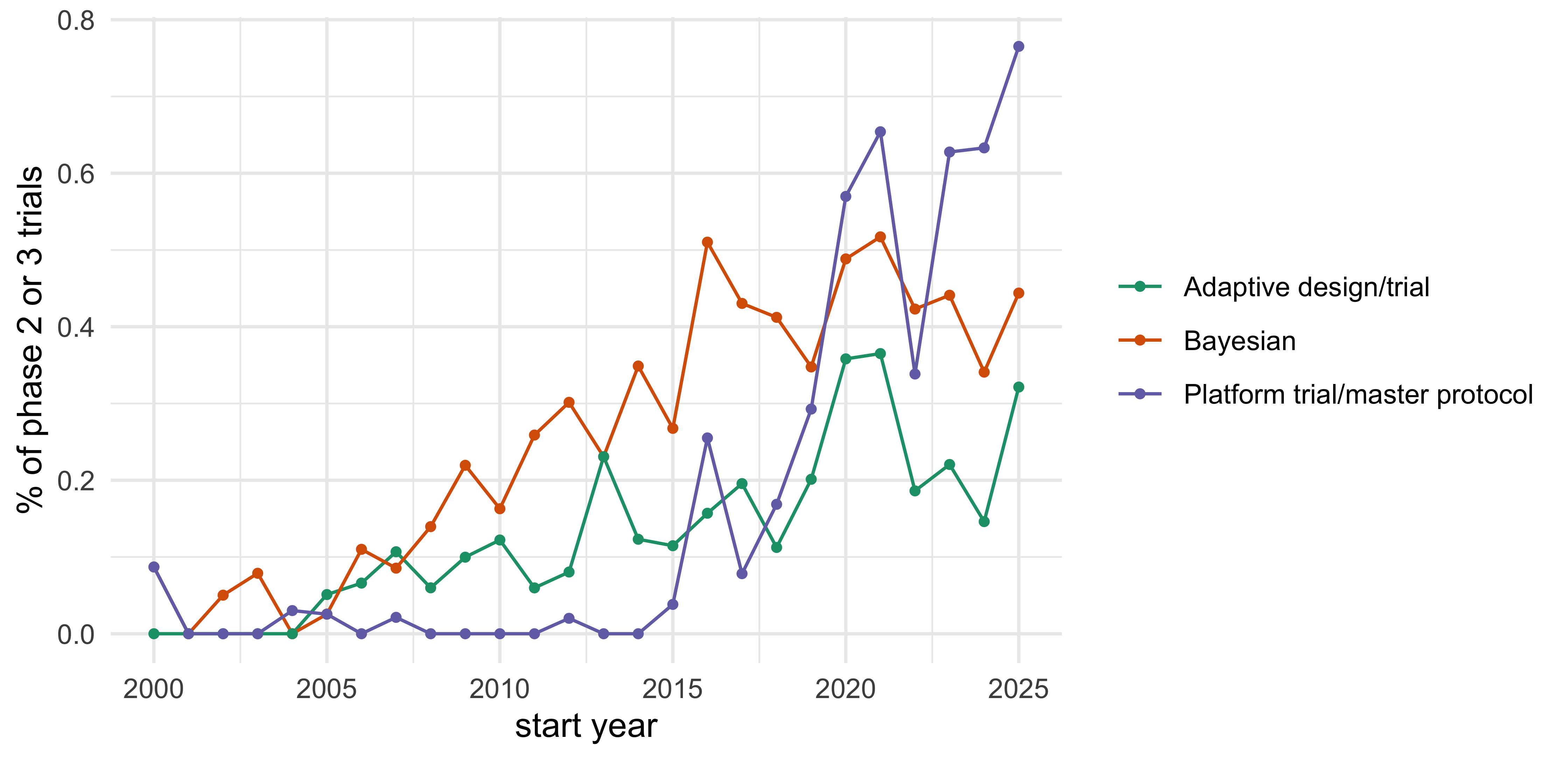
The registry suggests so, with large caveats. Figure 1.1 plots the share of interventional trials starting each year (phase 2 or 3 and combined phases) whose ClinicalTrials.gov record mentions Bayesian methods, adaptive designs or a platform or master protocol. In 2010, 8 of 4,912 phase 2 or 3 trials mentioned Bayesian (0.16 percent); in 2025 it was 29 of 6,534 (0.44 percent), nearly a tripling of the share. Platform or master-protocol trials went from 0 in 2010 to 50 in 2025 (0.77 percent of phase 2 or 3 starts).
Show the R code
keep <-c("Bayesian", "Adaptive design/trial", "Platform trial/master protocol")ggplot(subset(cc, term %in% keep), aes(year, share_pct, colour = term)) +geom_line() +geom_point(size =1) +scale_colour_brewer(palette ="Dark2") +labs(x ="start year", y ="% of phase 2 or 3 trials", colour =NULL) +theme_minimal()
Figure 1.1: Share of phase 2 or 3 interventional trials (including combined phases) starting each year whose ClinicalTrials.gov record mentions the term, 2000 to 2025. These are registry mention rates, not adoption rates: the search is free text, about 10 percent of Bayesian hits in a hand check of 20 records were false positives, many sponsors do not describe the design in the registry, terminology and registration practice change over time, and 2025 is incomplete. Downloaded 8 November 2026 (package dataset ctgov_counts).
The query is a text search, and in a hand check of 20 Bayesian records 18 truly used a Bayesian design or analysis, though most of those were Bayesian tools inside early-phase designs (BOIN, CRM, Bayesian safety monitoring) and not fully Bayesian confirmatory trials. Registries also under-report adaptive designs: in a review of registered trials, only 3 percent of a sample of adaptive trials known from the published literature were found by the registry search (Hatfield et al. 2016). Mentions increased between these cohorts, led by early phases and oncology, but changes in actual use cannot be separated from changes in reporting.
The counterweight
None of this says that a Bayesian design is automatically smaller or faster, and the book is built on saying where it is not. In the SELECT reconstruction the earlier decisions come from monitoring on the event grid at a bar that controls type I error, not from a lenient one. Against a single unadjusted look at a fixed level, the Bayesian bar is never lower without an informative prior, and the Bayes-factor bar is higher once \(I_n\tau^2\) exceeds about 42 (derived below; here \(I_n\) is the total information accumulated and \(\tau\) is the standard deviation of the prior on the effect under the alternative). And in a trial where the effect is modest, the scheduled design can win: in the REWIND reconstruction of Section 1.1 the Bayes rule decides earlier when it decides, but it decides less often. A sponsor should prefer a Bayesian design when the efficiency is real in that sponsor’s setting, and should be able to show it by simulation. The rest of the book is how.
1.4 A trial is a measurement and a decision
D. R. Cox, in Planning of Experiments(Cox 1958), described the setting of the clinical trial as one of “large uncontrolled variations.” In physics, once the apparatus is working, closely reproducible results emerge: the uncontrolled variation is small next to the effect being measured. A clinical trial lives in a different world. A patient’s outcome swings with the natural history of the disease, with the environment, with the psychological response to being treated, and with the supportive care received. The effect of a new drug, often only a modest improvement over existing therapy, has to be picked out from underneath all of that.
Everything in this book follows from that sentence. Because the variation between patients is large and cannot be removed, a single trial can never prove anything. It can only change what we believe, and then someone has to act on the changed belief: approve or not, continue or stop, give the next patient drug A or drug B. A trial is therefore two things at once. It is a measurement, and it is a decision. The traditional apparatus that most readers use every day was built to make the measurement honest and to put a fixed ceiling on one kind of wrong decision. It does that well. This book asks what changes when the decision is put in the foreground, and what the regulator will want to see when it is.
1.5 The traditional trial, fairly stated
Most readers can recite the traditional design, and it deserves a careful statement before anything is set against it, because it is a coherent and successful answer to a real problem.
The sponsor picks a primary endpoint and a treatment effect \(\theta\) that the trial should be able to detect. For a time-to-event endpoint, \(\theta = -\log \mathrm{HR}\), so that benefit is positive. The null hypothesis is that the new treatment is no better than control. The sponsor fixes a one-sided type I error rate \(\alpha\), conventionally \(0.025\), which is the same as the familiar two-sided \(0.05\) when only benefit counts. It also fixes power \(1-\beta\), say ninety percent, against the design alternative \(\theta\). A short calculation then gives the sample size, \[
I_n = \frac{(z_\alpha + z_\beta)^2}{\theta^2}, \qquad\text{which is}\qquad I_n = \frac{10.51}{\theta^2}\ \text{at } \alpha = 0.025,\ 1-\beta = 0.90,
\] where \(I_n\) is the total information required (for a time-to-event endpoint with one-to-one randomization each event carries information \(1/4\), so the number of events is \(4I_n\), as Chapter 9 shows) and \(z_\alpha\) is the upper \(\alpha\) quantile of the standard normal distribution. Patients are randomized one to one, because equal arms minimize the variance of the comparison for a given total. The protocol states in advance when the data will be analyzed, and the clinical study report (CSR) reports a point estimate, a confidence interval, and a p-value. The trial is “positive” if the p-value is below \(\alpha\).
Three features of this design are easy to underrate.
First, the type I error rate is a promise about the procedure, made before any data exist. If the drug does nothing, then over many trials run this way, at most a fraction \(\alpha\) will declare success. That promise is checkable without anyone’s opinion about how likely the drug is to work, and it is the reason the design is trusted by regulators who must deal with sponsors who have every incentive to see a benefit.
Second, the promise survives repeated use only if the analysis plan is fixed in advance. If the trial may be examined before it ends, the right to look is paid for. A group sequential design spends part of \(\alpha\) at each interim analysis according to a pre-specified function (Lan and DeMets 1983), and the boundaries of O’Brien and Fleming (O’Brien and Fleming 1979) are very strict early and nearly the fixed-sample value at the end. If the trial has several arms, doses, endpoints or subgroups, the level is divided among the contrasts (Bonferroni, Holm) or passed along a pre-specified graph, so that the chance of any false claim stays at \(\alpha\). The apparatus is complete and well understood, and ICH E9 describes it at length.
Third, the regulatory machinery has grown around it. Statisticians at sponsors and at the regulator share a vocabulary, a set of software tools, and decades of precedent. A reviewer who sees “one-sided \(\alpha = 0.025\), two interim looks with Lan-DeMets O’Brien-Fleming spending, graphical multiplicity procedure” knows what is meant without reading further. Nothing in this book is a reason to abandon that shared language. The question is which parts of the design can be improved, at what price, and in what terms a regulator will accept the improvement.
What the apparatus costs
Each component has a price that is rarely itemized, and the Bayesian case rests on stating those prices exactly. Most of the numbers below are computed in the code that follows; the combined four-look, six-contrast boundary of about 5.3 and the interval of 0.01 to 0.51 are quoted, not computed.
Show the R code
K <-4; z <-qnorm(0.975)ob <-gs_boundary(K, 0.025, "obf"); po <-gs_boundary(K, 0.025, "pocock")pl <-c("Four looks, one-sided 0.025", "Bayes bar against information n")d1 <-data.frame(panel =factor("Four looks, one-sided 0.025", pl), x =rep(1:K, 2), z =c(ob, po), rule =rep(c("O'Brien-Fleming", "Pocock"), each = K))n <-seq(2, 400, length.out =400)d2 <-data.frame(panel =factor("Bayes bar against information n", pl), x = n, z =sqrt(log(n)), rule ="Bayes: sqrt(log n)")ggplot(rbind(d1, d2), aes(x, z, colour = rule)) +geom_line() +geom_point(data = d1) +geom_hline(yintercept = z, linetype =3) +facet_wrap(~panel, scales ="free_x") +scale_colour_brewer(palette ="Dark2") +labs(x ="analysis (left), information n (right)", y ="critical z", colour =NULL) +theme_minimal()
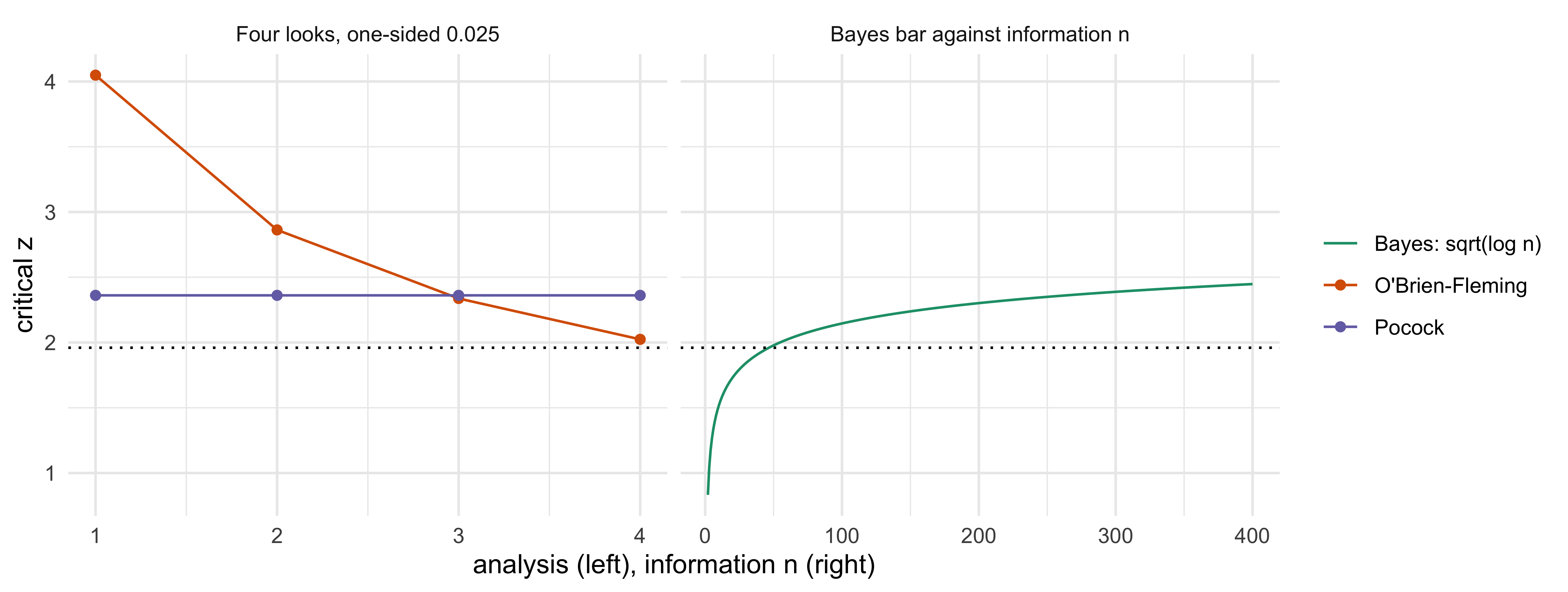
Figure 1.2: Critical values on the standardized (z) scale. Left: four equally spaced looks at one-sided level 0.025. The fixed-sample value is 1.96. A naive repeated test at 1.96 has an overall one-sided error of about 0.063, so the boundaries must be raised: O’Brien-Fleming is very high early, Pocock is flat at 2.36. Right: the value of the Bayes factor rule, sqrt(log n), against the fixed value 1.96. In the logarithmic approximation the two cross at n = exp(1.96^2), about 46.6, where n is information times prior variance (a unit-information prior); the exact mixture boundary crosses at about 41.6, and at the prior scale used later in the book the crossing needs far more information (Chapter 11).
A sample size fixed in advance. The formula \(I_n = 10.51/\theta^2\) commits the trial to a guess \(\theta\). If the true effect is larger than the guess, the trial runs longer than it needed to and patients stay on the inferior arm for no reason. If it is smaller, power is below target, although the estimate and confidence interval may remain informative. The cost of the guess is paid in one direction or the other, and the formula has no way to adjust.
An error budget spent in advance. For four equally spaced analyses, the O’Brien-Fleming boundaries in Figure 1.2 run from about 4.05 at the first look down to about 2.02 at the last. A trial that stops at the first interim look must have produced a result four standard errors from zero. That is a very high bar for a treatment effect of the size a confirmatory trial usually studies. What the sponsor purchases is the right to stop early if the drug is spectacular, and the price is paid by every trial where the drug is merely good. Testing naively at 1.96 at each of four looks does not work either: the overall one-sided error is about 0.063, more than twice the nominal 0.025. That is the problem the spending function solves.
A multiplicity correction applied at the end. With four arms there are six pairwise contrasts. A Bonferroni correction takes the level to \(0.025/6 = 0.00417\), with a critical value of 2.64 in place of 1.96. Combine that with four looks and the first interim boundary moves to about 5.3. The correction is conservative because it must be valid whatever the correlation between contrasts and whatever the truth, and it treats a contrast the same whether or not the other arms resemble it.
In small trials, an appearance of decisiveness. In dose-finding, the standard design enrolls twelve to thirty patients. Observing one toxicity in six patients at the recommended dose, with a \(\mathrm{Beta}(0.25, 0.75)\) prior, leaves a ninety-five percent posterior interval for the toxicity probability running from about 0.01 to 0.51 (Polson and Sokolov 2026a). A procedure that returns an interval that wide has not identified a dose, though the protocol will name one. We return to this in Chapter 17.
None of these costs is a flaw in the logic of the traditional design. They are what it costs to deliver the one promise, that of a fixed ceiling on false positives, under every circumstance in which the design might be used.
1.6 From a test to a decision
At any moment in a trial, someone with authority to act (a sponsor, a data monitoring committee, a regulator) has a small set of options. Continue enrolling. Stop for futility. Stop because the drug has clearly worked. Take the drug to the regulator. Each option has consequences for patients inside the trial, for patients outside it who will or will not receive the drug later, and for the sponsor. A hypothesis test answers a narrower question, “is the data surprising if the drug does nothing?”, and leaves the rest to judgment outside the statistics. The decision framework tries to put that judgment inside the model, where it can be inspected.
It needs three ingredients.
A prior. A probability distribution \(\pi(\theta)\) for the treatment effect before the trial, summarizing what is known from earlier phases, from related drugs, from mechanism, and from the history of how often drugs entering a confirmatory trial turn out to work.
A model for the data. The likelihood \(p(y \mid \theta)\) is the same as in the traditional analysis. Nothing about the Bayesian approach changes how the outcome data are modeled. After the data arrive, Bayes’ rule turns the prior into a posterior \(\pi(\theta \mid y)\).
A utility (or loss). A statement of what the possible outcomes are worth. Approving a drug that works gains something, approving one that does not harms the patients who take it and wastes resources, and failing to approve a good drug loses what those patients would have gained. Every additional month of the trial and every additional patient randomized to the inferior arm carries a cost.
The decision rule follows. At a terminal analysis, suppose the only choices are to approve or to reject. Act when the posterior expected loss of approving is smaller than that of rejecting. Suppose that approving a drug that does not work costs \(L_{\mathrm{I}}\), that failing to approve a drug that does work costs \(L_{\mathrm{II}}\), and that correct decisions cost nothing. If \(p\) is the posterior probability that the drug works, the expected loss of approving is \((1-p)L_{\mathrm{I}}\) and the expected loss of not approving is \(p\,L_{\mathrm{II}}\). Approval is better when \[
p > \frac{L_{\mathrm{I}}}{L_{\mathrm{I}} + L_{\mathrm{II}}}.
\tag{1.1}\] The posterior probability must exceed a threshold that depends on the ratio of the two costs, and nothing else. If a false approval is thirty-nine times as costly as a missed drug, the threshold is \(39/40 = 0.975\). The one-sided \(\alpha = 0.025\) of the traditional design is, in this reading, an implicit statement of that ratio. An interim decision is harder: it must also compare both terminal losses with the sampling cost and the expected value of continuing, so the displayed threshold alone is not an interim stopping rule (Chapter 15).
Show the R code
# Flat prior on the effect, normal likelihood: posterior is N(est, se^2), so# Pr(theta > 0 | data) = pnorm(est / se). Threshold = L_I / (L_I + L_II).r <-c(1, 9, 39, 99); t <- r / (r +1)knitr::kable(data.frame(r, t, qnorm(t)), digits =c(0, 3, 2), col.names =c("Cost ratio (false approval : missed drug)", "Approve when posterior probability exceeds", "Equivalent z"), align ="rrr")
Cost ratio (false approval : missed drug)
Approve when posterior probability exceeds
Equivalent z
1
0.500
0.00
9
0.900
1.28
39
0.975
1.96
99
0.990
2.33
With a flat prior and a normal likelihood the posterior probability that the effect is positive equals one minus the one-sided p-value, so approving when it exceeds \(0.975\) is the same as rejecting when \(p < 0.025\). The two designs agree numerically on that analysis, and that is the point of departure. A traditional analysis at the end of a fixed trial with no interim looks and one primary contrast is already a Bayesian decision with a flat prior and a particular cost ratio. The disagreements begin when there is more than that: looks, multiple arms, historical information, a cost per patient.
The three things a protocol fixes
Seen this way, every protocol, traditional or Bayesian, fixes three things before the first patient is randomized.
What is known going in. In the traditional protocol this is implicit: the design alternative \(\theta\) and a variance. In a Bayesian protocol it is explicit, as a prior, and the protocol must justify it (Chapter 8).
What will count as success. In the traditional protocol, a p-value below \(\alpha\) with adjustments. In a Bayesian protocol, a posterior criterion such as \(\Pr(\delta > a \mid \text{data}) > c\), where \(\delta\) is the treatment effect, \(a\) is the smallest effect that matters, and \(c\) is the posterior probability threshold, the form that appears in the FDA draft guidance (U.S. Food and Drug Administration 2026).
What the data-generating process allows the sponsor to do along the way. The sample size, the interim analyses, the permitted adaptations, the allocation ratio. These are the protocol’s operating rules, and they determine the operating characteristics: the probability of declaring success under each possible truth.
The third item is where the regulator’s interest is concentrated, and it is why the book returns so often to simulation. A regulator does not need to share a sponsor’s prior or utility to evaluate a design. It can ask what the design does: under the null, how often does it declare success? Under a plausible alternative, how often does it succeed and how many patients does it use? A Bayesian design is judged, in practice, by the same standard as a traditional one, with the trial simulated many times under pre-specified truths (Chapter 14). The Bayesian approach changes how the rule is built, not the court in which it is judged.
Two kinds of “decision maker”
There is a second reason to put the decision in front. Two different people are deciding, and they are not asking the same question. In a study of the prostate cancer choices of two high-profile patients (Polson and Sokolov 2026b), we found that the physician and the patient reasoned about different quantities. The physician, trained to think in terms of the population and the most likely disease state, reasons from the modal case: the cancer is probably low risk, the patient can probably be cured by something not too aggressive, so why be aggressive for a small gain in cure probability? The patient, who has one life and one decision, reasons about the whole posterior, including the thin tail in which the disease has spread. A colleague of the first patient wrote that this is exactly the distinction: “It’s different to think of things in population terms (and for other people) than to think about them as an individual patient with one life.” Both patients recognized that the published risk estimate was a point estimate with known calibration error, and that it should propagate into the decision rather than be treated as exact.
The same asymmetry shows up in trial design. The regulator and the sponsor think at the level of the population: will the drug meet the standard? The patient in the trial, and the patient who will be prescribed the drug afterwards, bears the consequences one at a time. A design that lets the trial stop earlier when the posterior is decisive, or that allocates fewer patients to a losing arm, is a design that takes the second perspective seriously. Using the same decision-theoretic language for both is the attraction of the framework, and a utility function is where the disagreement between them can be written down and argued about instead of left implicit.
1.7 Preview: the thesis and four mechanisms
The thesis of this book can be stated in two sentences. A regulator approves a drug on evidence that meets a legal standard, and a Bayesian adaptive design can meet that standard sooner and with fewer patients exposed to inferior arms. The saving comes from monitoring, from handling multiple arms jointly, and from using prior information, and it does not come from a lower bar: against a single unadjusted analysis, the Bayesian bar is never lower without an informative prior, and the Bayes-factor bar is higher once \(I_n\tau^2\) exceeds about 42.
That last claim is the one a skeptical reader should test first, so here is the arithmetic. A fixed-sample test at one-sided level \(0.025\) demands a standardized score of \(z_\alpha = 1.96\) whatever the amount of information. The Bayes-factor rule, which with even prior odds and equal costs acts when the posterior probability of the alternative exceeds that of the null, demands, approximately, a score whose square exceeds the logarithm of the accumulated information \(n\). This logarithmic penalty is sometimes called the Ockham penalty: a hypothesis that could explain any data is rewarded less than one that made a sharp prediction, and the reward shrinks as the amount of data grows (Chapter 7). For the stated mixture prior and \(b = 1\) the exact boundary is \(Z_n^2 \ge (1 + 1/q)\log(1+q)\) with \(Z_n > 0\) and \(q = I_n\tau^2\) (information times prior variance); on the score scale the logarithmic approximation of the bar is \(\sqrt{\log n}\). The exact boundary crosses \(1.96^2\) at \(q \approx 41.6\), and the approximation \(n = e^{1.96^2} \approx 46.6\) shown in the right-hand panel of Figure 1.2 overstates the crossing (Chapter 11). Beyond the crossing the Bayes-factor bar is higher than the fixed-sample bar (Polson and Sokolov 2026a). SELECT at the prior scale \(\tau = 0.25\) has \(q = 1270/64 \approx 19.8\), below the crossing. Holding the Bayes-factor threshold fixed can increase the required information, whereas calibrating a single-analysis rule to the same type I error can instead reproduce the conventional test, and Chapter 9 does the calculation carefully. Three rules are called Bayesian in this book and they should not be confused: the flat-prior posterior threshold of equation Equation 1.1 (numerically a one-sided test), the Bayes-factor rule just described, and the continuously monitored rule calibrated to a type I error of 0.025 (a posterior probability threshold of about \(p^* = 0.995\) in the SELECT reconstruction of Chapter 21). The saving claimed in this book belongs to the third.
So where does the saving come from? Claims that Bayesian designs need fewer patients draw on four mechanisms that are usually run together. They differ in how much they assume, and the book keeps them apart (Polson and Sokolov 2026a).
M1. The deviation scale. The deviation scale is the size of the standardized score that a rule must see before it acts, as a function of the amount of data. A decision rule that must be valid at every possible stopping time, as an anytime-valid e-value rule is (a rule whose false-positive guarantee holds however often and whenever the data are examined), pays a surcharge on top of the logarithmic term, which for the symmetric normal mixture is approximately \(2\log(1/\alpha)\) in squared standardized units when information is large (exactly \((1 + 1/q)\,2\log(1/\alpha)\), with \(q = I_n\tau^2\)). In plain terms the surcharge is the extra evidence demanded in return for the right to look at any time without planning the looks. The uncalibrated Bayes-factor rule does not pay it. Asymptotically the surcharge is about seventy percent of the boundary term \(10.51\) of a conventional trial, a comparison of boundary terms and not an exact sample-size identity; calibration narrows the realized gap (Chapter 11 and Chapter 12). The surcharge is a property of this normal-mixture construction, not a universal cost of anytime validity, and it is not free.
M2. One calibrated threshold for monitoring, and shrinkage for estimation. A group sequential design pays for looking by raising the early boundaries, and Bonferroni pays for several contrasts by raising them again. A Bayesian analysis can monitor continuously with a single calibrated threshold (about 0.995 rather than 0.975 in SELECT), which is another monitoring boundary and not an escape from monitoring costs. For several arms it can shrink the estimates toward a common mean (pulling each arm’s estimate toward the average of all the arms, more strongly when the arm has little data). Shrinkage improves estimation, but it does not by itself control the familywise error rate, particularly under partial null configurations, so the complete confirmatory decision rule still needs its error evaluated and, where required, calibrated. Any saving must be shown between designs with comparable error and power (Chapter 10, Chapter 11).
M3. Informative priors. If effects reaching a confirmatory trial are known to be small (Sokolova, Sokolov, and Polson 2026), a prior concentrated on small effects carries real information, formally equivalent to a number of pseudo-observations whose size can be reported as a prior effective sample size (Morita, Thall, and Müller 2008). It is genuine when the prior is right and a bias when it is wrong, so it must come with a sensitivity analysis (Chapter 8, Chapter 19).
M4. Optimal stopping under a sampling cost. When each patient carries a cost, the best Bayes rule is found by working backward from the end of the trial (a dynamic program), and the continuation region (the set of interim results for which the trial keeps going) narrows as the horizon approaches, so its expected sample size is typically below that of a fixed design with comparable error rates (Chapter 15).
NoteTechnical note: the arithmetic of M1 and M2
With \(q = I_n\tau^2\), the exact symmetric normal-mixture bar is \(Z_n^2 \ge (1 + 1/q)(\log(1+q) + 2\log b)\) with \(Z_n > 0\) for a one-sided claim, and the e-value bar is the same with \(b = 1/\alpha\). The exact surcharge over the Bayes-factor bar at \(b = 1\) is therefore exactly \((1 + 1/q)\,2\log(1/\alpha)\), whose large-information approximation is \(2\log(1/\alpha) = 7.38\) at \(\alpha = 0.025\). The seventy percent quoted above compares \(7.38\) with \((z_\alpha+z_\beta)^2 = 10.51\) for a conventional trial at 90% power; it compares boundary terms asymptotically and is not a predicted sample-size reduction (subtracting the sample-size equations adds a positive \(\log\) term). We do not quote information ratios between the first O’Brien-Fleming boundary and the uncalibrated Bayes-factor bar, because that compares a calibrated rule with an uncalibrated one.
Two of the four mechanisms (M2 and M4) rest on structure that a regulator can verify by simulation. One (M3) rests on a judgment that must be defended. One (M1) is a mathematical fact, under stated approximations, that comes with a trade-off. Each is quantified in the chapters named, and the case studies of Chapter 21 apply them to real trials, among them SELECT, the semaglutide cardiovascular outcomes trial of 17,604 patients that read out on 1,270 primary events (Lincoff et al. 2023), and the four-arm ulcer-surgery trial in which Novick and Grizzle (Novick and Grizzle 1965) made the original Bayesian case for treating several treatments together. The ulcer trial, taken up in Chapter 10, is worth previewing because it shows multiplicity and repeated analysis together defeating the frequentist reading of what looked like a real effect.
What we claim and what we do not
We claim that a Bayesian design can decide sooner when it is monitored, that the reason is the structure of the monitoring and of the multiple comparisons rather than a lenient threshold, and that the magnitude can matter in patient-years. We do not claim that it dominates. The surcharge a Bayesian rule declines to pay buys a real guarantee: a sponsor who cannot commit to a monitoring plan should pay it. A sponsor who runs a single well-powered look has no reason to pay an anytime-valid surcharge at all, and should use the fixed-sample test. The REWIND trial of dulaglutide is an example in which the scheduled design wins, and Chapter 21 says why. Equally, every Bayesian gain has a price (a prior that must be defended, simulations that must be run, a design that is more work to specify), and the price must be itemized in the currency the regulator accepts, which is simulated operating characteristics under a pre-specified design.
1.8 What the regulator needs, and what it does not
The regulatory standard is easy to misread in either direction. The statute says that a drug may be approved if there is substantial evidence that it has the effect claimed, and defines substantial evidence by reference to adequate and well-controlled investigations (United States Congress 1962). The regulation 21 CFR 314.126 lists what makes an investigation adequate and well-controlled (objectives, a valid control, bias-minimizing assignment and assessment, reliable response measures, and an adequate analysis; the full list is in Chapter 3) (U.S. Food and Drug Administration 2024). Nowhere does the statute or the regulation say “p-value” or “type I error.” A test of significance is the method that ICH E9 describes and that decades of practice have settled on, but the legal standard is evidence, not a procedure.
This has two consequences that run through the book. First, a Bayesian design is not exotic in law. It is a different way of showing that the evidence is substantial, and the FDA’s 2026 draft says so by listing three routes to a success criterion: calibration to type I error, direct reading of the posterior, and a benefit-risk decision rule (U.S. Food and Drug Administration 2026). Only the first is tied to type I error. Because the draft is a draft, it describes what the agency is prepared to discuss, not what it requires. Second, the standard is about the whole design: a valid comparison with a control, measures against bias, and a pre-specified analysis, usually achieved through randomization and blinding (the regulation also recognizes historical controls and settings where blinding is not feasible). A Bayesian posterior computed from a trial without a valid comparison and bias control does not meet 314.126 however sophisticated the model. Bayesian methods change the analysis and the adaptation rules, and they do not change the need for a fair comparison. Chapter 5 explains why a Bayesian still randomizes.
ICH E8(R1) adds a point that fits this book’s emphasis on design. It asks sponsors to build quality into the trial from the start, by identifying the factors that are critical to the decision the trial will support and by concentrating effort on those (International Council for Harmonisation 2021). That is the decision framing in regulatory language: if you cannot say which decision the trial supports and which features of the trial bear on it, you cannot design it well. A Bayesian adaptive protocol makes those statements explicit, since the prior, the success criterion and the operating rules are all written down, and in that respect the Bayesian approach has an affinity with quality by design. ICH E9 and its addendum E9(R1) (International Council for Harmonisation 1998, 2019) remain the statistical baseline, and the FDA adaptive-design guidance of November 2019 (U.S. Food and Drug Administration 2019) is the final guidance that allows pre-planned adaptations provided they preserve the integrity of the trial and control the chance of a false conclusion. All of these are described in Chapter 3.
The flat-prior equivalence of the Bayes rule and the one-sided p-value is derived for the normal model in Chapter 7, where it is also contrasted with a point null.
1.9 A short history
The decision-theoretic view of trials is as old as the randomized trial. Thompson asked in 1933 for the probability that one treatment is better than another and proposed allocating patients accordingly (Thompson 1933). Wald’s sequential analysis came from the wartime problem of sampling only as much as needed (Wald 1947). Grundy, Healy and Rees posed the economic choice of the amount of experimentation in 1956 (Grundy, Healy, and Rees 1956), and Raiffa and Schlaifer’s 1961 decision theory supplied the preposterior analysis (Raiffa and Schlaifer 1961). Anscombe and Colton observed in 1963 that a trial is run to inform the treatment of a much larger population of future patients, and derived trial sizes from that population rather than from an error rate (Anscombe 1963; Colton 1963). Novick and Grizzle gave a Bayesian analysis of a four-arm surgical trial in 1965 (Novick and Grizzle 1965). Cornfield gave a Bayesian sequential test for clinical trials in 1966, and set out the Bayesian outlook for trials in 1969, with a prior probability on the null hypothesis and relative betting odds as the summary of the evidence (Cornfield 1966, 1969), and with Halperin and Greenhouse an adaptive allocation procedure (Cornfield, Halperin, and Greenhouse 1969); Lindley’s decision theory (Lindley 1985) gives the general framework. Berry restated the case for Bayesian interim analysis in 1985 and spent the following decades building Bayesian adaptive designs (Berry 1985), including decision-theoretic stopping boundaries with Ho (Berry and Ho 1988). Lewis and Berry evaluated Bayesian decision-theoretic designs by their classical operating characteristics (Lewis and Berry 1994), the idea behind the calibration route that the FDA draft describes (Chapter 3). Whitehead’s “case for frequentism” is the standard statement of the opposing view (Whitehead 1993). Inside the pharmaceutical industry, the Basel group of Racine, Grieve, Flühler and Smith showed that Bayesian methods could be used routinely in drug development (Racine et al. 1986). In January 2026 the FDA issued draft guidance on Bayesian methodology for drugs and biologics (U.S. Food and Drug Administration 2026), and the EMA released a concept paper on Bayesian methods for consultation (European Medicines Agency, Methodology Working Party 2026); the regulatory history and the response to the FDA draft are in Section 3.5.2 and Section 3.5.4.
The objections deserve their strongest form. The prior can decide the answer. Prior choice can change the conclusion, and the FDA draft recommends prespecified sensitivity analyses across reasonable alternative priors, with the influence of the primary prior quantified and justified (answered by sensitivity analysis and the effective sample size of Chapter 8). The type I error rate of a Bayesian rule is not controlled by the Bayes calculation itself (answered by calibration through simulation, Chapter 14). Interim peeking at accumulating data can bias the trial and the people who run it (answered by firewalls and prespecification, Chapter 11). And a Bayesian design is harder to review than a fixed-sample trial (answered, so far as it can be, by the simulation report and by the protocol content of Chapter 23). Berry, a leading Bayesian designer, wrote of the promise and the caution of adaptive trials (Berry 2011), Bauer and colleagues reviewed the opportunities and pitfalls of confirmatory adaptive designs (Bauer et al. 2016), and Lee and Chu reviewed Bayesian trials in action (Lee and Chu 2012). The response to the 2026 draft guidance repeats these objections in current form (Section 3.5.4).
1.10 A map of the book
The book is built in five parts, and each starts from what the reader already does.
Part I, Trials, Decisions, and Regulation. This chapter frames the problem. Chapter 2 follows a drug through phases I to IV and shows where each kind of evidence, and each kind of error, enters. Chapter 3 is the map of the regulatory texts that every later chapter cites: statute and regulation, the ICH guidelines, the FDA guidances on adaptive designs, Bayesian methods, master protocols and substantial evidence, and the programs through which sponsors talk to the agency.
Part II, Basics. These chapters start from first principles, so that a reader who has forgotten testing can follow. Chapter 4 rebuilds the two-group comparison, the p-value, error rates and power from simulation. Chapter 5 explains why we allocate by chance, how it is done, and why a Bayesian still does it. Chapter 6 introduces prior, likelihood and posterior and repeats the two-group comparison the Bayesian way. Chapter 7 compares the evidence from p-values and Bayes factors and shows how the posterior probability criterion of the FDA draft reads. Chapter 8 is about choosing and defending a prior, which is where most regulatory discussion is concentrated.
Part III, The Standard Apparatus Reconsidered. Each chapter takes one component of the traditional design and asks what the decision framework says about it. Chapter 9 treats sample size and power, with the Bayesian replacement for the textbook formula. Chapter 10 treats multiple comparisons and shrinkage, including the ulcer trial. Chapter 11 treats interim looks and the three deviation scales that give the surcharge. Chapter 12 treats anytime-valid inference, which is a frequentist answer to the problem of looking at any time. Chapter 13 applies the same machinery to safety signals and safety monitoring, with the rofecoxib cumulative record as the running example.
Part IV, Bayesian Adaptive Designs. These chapters build the designs. Chapter 14 shows how to calibrate a Bayesian rule to type I error and how to write the simulation report the FDA draft and ICH E20 (draft, Step 2, June 2025) ask for. Chapter 15 treats predictive probability, futility and stopping. Chapter 16 treats response-adaptive randomization and bandits, including the controversies. Chapter 17 treats dose finding and dose optimization. Chapter 18 treats time-to-event endpoints, where events rather than patients carry the information. Chapter 19 treats borrowing of information from other trials, external controls and pediatric extrapolation. Chapter 20 treats master protocols and platform trials.
Part V, From Design to Approval.Chapter 21 applies the machinery to real trials, with the semaglutide cardiovascular outcomes trial SELECT, the dulaglutide trial REWIND, and TRAILBLAZER-ALZ 2 in Alzheimer’s disease. It also covers the BNT162b2 vaccine trial with its Bayesian success criterion, and it values the saving in patient-years and money. Chapter 22 reanalyzes four landmark trials (GUSTO, EOLIA, ANDROMEDA-SHOCK and RECOVERY) and says what a reanalysis can and cannot claim. Chapter 23 turns the machinery into the document: the protocol table, the statistical analysis plan, the simulation report, the data monitoring committee charter, and what to say to the agency and when.
The appendices give the notation (Appendix A), a list of regulatory documents and programs with status and links (Appendix B), and the software and code used (Appendix C).
Three conventions hold throughout. The traditional version comes first, and the Bayesian version of the same decision follows on the same numbers, followed by a side-by-side comparison of what changes in the protocol, what stays the same, and what the regulator will ask. One-sided \(\alpha = 0.025\) is the default level, and two-sided is stated whenever it is used. And whenever a Bayesian design is said to be better, the book says what it costs and where the traditional design is the better choice.
TipIn the protocol
Whatever the design, the protocol and statistical analysis plan should answer five questions in so many words. What decision does this trial support, and who makes it? What prior information is used, if any, and why? What is the success criterion, in a form that can be evaluated by computer? What are the permitted adaptations and the stopping rules? What are the operating characteristics (type I error, power or probability of success, expected sample size) under pre-specified scenarios, and how were they computed? A traditional protocol answers most of these implicitly. A Bayesian protocol must answer them aloud, and that is as much of a benefit as it is a burden.
TipTry it in the lab
Open Module 12, “Decisions: what Type I control costs” (https://nytel.ai/testing/12-decisions.html). Before you touch a control, predict what happens to the power of a fixed trial when the number of looks goes from one to four and the number of Bonferroni tests from one to six. Then set the sliders in section B and compare. In section A, move the cost ratio from 39:1 to 9:1 and see how the threshold \(L_{\mathrm{I}}/(L_{\mathrm{I}}+L_{\mathrm{II}})\) in Equation 1.1 changes.
1.11 In practice
Three regulatory episodes show the decision framing at work. The detailed accounts, with thresholds and sources, are in Section 3.11, and the BNT162b2 calculation is worked in Section 6.12.
A Bayesian criterion and a frequentist guarantee are not alternatives. The BNT162b2 posterior bar was tuned by simulation to a one-sided type I error of 2.5 percent (Chapter 14).
The number of trials needed is itself a threshold. REBYOTA’s two posterior thresholds stood for one trial and for two, and the stricter one, for two trials, was not met (Chapter 19).
A decision rule on a predictive probability stops arms early. I-SPY 2 graduated neratinib on 115 evaluable patients (127 randomized), and the final predictive probability fell below the bar because the last outcomes arrive after the decision (Chapter 15).
Key points
A clinical trial works against large uncontrolled variation between patients (Cox). It measures a treatment effect and, at the same time, supports a decision to approve, continue or stop.
The traditional design (fixed \(I_n = 10.51/\theta^2\) for \(\alpha = 0.025\) and ninety percent power, one-to-one randomization, spending for looks, multiplicity correction, a p-value in the CSR) is coherent. Its central strength is a fixed ceiling on the false-positive rate, whatever the prior.
A Bayesian trial adds a prior, a utility and a rule: at a terminal analysis, approve when the posterior expected loss of approving is smaller than that of rejecting (an interim decision must also weigh the value of continuing). With a flat prior and one look this is the same decision as a one-sided test, with a cost ratio of 39 to 1 at \(\alpha = 0.025\).
The law asks for substantial evidence from adequate and well-controlled investigations (FD&C Act 505(d), 21 CFR 314.126), not for a statistical philosophy. Bayesian methods change the analysis and the adaptation rules and leave the need for a fair, randomized, blinded comparison where it was.
The saving from a Bayesian design comes from four mechanisms: the deviation scale, a single calibrated threshold for monitoring (with shrinkage for estimation, not a substitute for error control), informative priors, and optimal stopping. It does not come from a lower bar. Once information times prior variance exceeds about 42 (\(I_n\tau^2 \gtrsim 42\) for the exact mixture boundary; the logarithmic approximation gives 46.6) the Bayes-factor bar is higher than a single unadjusted look.
Each gain has a price, and the price is stated in simulated operating characteristics under a pre-specified design.
NoteDiscussion questions
Pick a trial you have worked on. Write down the three things its protocol fixed: what was known going in, what counted as success, and what the sponsor could do along the way. Which were stated explicitly and which were left implicit?
A one-sided \(\alpha = 0.025\) corresponds to a cost ratio of 39 to 1 between a false approval and a missed drug. In what disease settings would you argue for a different ratio, and who should decide it?
Explain in your own words why, with a flat prior and a single look, a posterior probability above \(0.975\) and a one-sided p-value below \(0.025\) are the same rule. What has to be added to the trial for the two to disagree?
The Bayes-factor bar is higher than 1.96 once \(I_n\tau^2\) exceeds about 42, a crossing that SELECT at \(\tau = 0.25\) does not reach. Under what circumstances would a sponsor still be right to choose a Bayesian design? Under what circumstances would a single fixed-sample look be the better choice?
The physician in the prostate cancer example reasons from the modal state and the patient from the posterior. Where in a clinical trial does the same difference arise between the sponsor, the regulator and the patient?
Bauer, Peter, Frank Bretz, Vladimir Dragalin, Franz König, and Gernot Wassmer. 2016. “Twenty-Five Years of Confirmatory Adaptive Designs: Opportunities and Pitfalls.”Statistics in Medicine 35 (3): 325–47. https://doi.org/10.1002/sim.6472.
Berry, Donald A. 1985. “Interim Analyses in Clinical Trials: Classical Vs. Bayesian Approaches.”Statistics in Medicine 4 (4): 521–26.
Berry, Donald A., and Chih-Hsiung Ho. 1988. “One-Sided Sequential Stopping Boundaries for Clinical Trials: A Decision-Theoretic Approach.”Biometrics 44 (1): 219–27. https://doi.org/10.2307/2531909.
Colton, Theodore. 1963. “A Model for Selecting One of Two Medical Treatments.”Journal of the American Statistical Association 58 (302): 388–400. https://doi.org/10.1080/01621459.1963.10500853.
Cornfield, Jerome. 1966. “A Bayesian Test of Some Classical Hypotheses, with Applications to Sequential Clinical Trials.”Journal of the American Statistical Association 61 (315): 577–94. https://doi.org/10.1080/01621459.1966.10480890.
Cornfield, Jerome, Max Halperin, and Samuel W. Greenhouse. 1969. “An Adaptive Procedure for Sequential Clinical Trials.”Journal of the American Statistical Association 64 (327): 759–70. https://doi.org/10.1080/01621459.1969.10501010.
Cox, D. R. 1958. Planning of Experiments. New York: John Wiley & Sons.
DiMasi, Joseph A., Henry G. Grabowski, and Ronald W. Hansen. 2016. “Innovation in the Pharmaceutical Industry: New Estimates of R&D Costs.”Journal of Health Economics 47: 20–33. https://doi.org/10.1016/j.jhealeco.2016.01.012.
Gerstein, Hertzel C., Helen M. Colhoun, Gilles R. Dagenais, Rafael Diaz, Mark Lakshmanan, Prem Pais, Jeffrey Probstfield, et al. 2019. “Dulaglutide and Cardiovascular Outcomes in Type 2 Diabetes (REWIND): A Double-Blind, Randomised Placebo-Controlled Trial.”The Lancet 394 (10193): 121–30. https://doi.org/10.1016/S0140-6736(19)31149-3.
Grundy, P. M., M. J. R. Healy, and D. H. Rees. 1956. “Economic Choice of the Amount of Experimentation.”Journal of the Royal Statistical Society, Series B 18 (1): 32–49. https://doi.org/10.1111/j.2517-6161.1956.tb00207.x.
Hatfield, Isabella, Annabel Allison, Laura Flight, Steven A. Julious, and Munyaradzi Dimairo. 2016. “Adaptive Designs Undertaken in Clinical Research: A Review of Registered Clinical Trials.”Trials 17: 150. https://doi.org/10.1186/s13063-016-1273-9.
Lan, K. K. Gordon, and David L. DeMets. 1983. “Discrete Sequential Boundaries for Clinical Trials.”Biometrika 70 (3): 659–63.
Lee, J. Jack, and Caleb T. Chu. 2012. “Bayesian Clinical Trials in Action.”Statistics in Medicine 31 (25): 2955–72. https://doi.org/10.1002/sim.5404.
Lewis, Roger J., and Donald A. Berry. 1994. “Group Sequential Clinical Trials: A Classical Evaluation of Bayesian Decision-Theoretic Designs.”Journal of the American Statistical Association 89 (428): 1528–34. https://doi.org/10.1080/01621459.1994.10476893.
Lincoff, A. Michael, Kirstine Brown-Frandsen, Helen M. Colhoun, John Deanfield, Scott S. Emerson, Sille Esbjerg, Soren Hardt-Lindberg, et al. 2023. “Semaglutide and Cardiovascular Outcomes in Obesity Without Diabetes.”New England Journal of Medicine 389 (24): 2221–32. https://doi.org/10.1056/NEJMoa2307563.
Lindley, Dennis V. 1985. Making Decisions. 2nd ed. London: Wiley.
Moore, Thomas J., James Heyward, Gerard Anderson, and G. Caleb Alexander. 2020. “Variation in the Estimated Costs of Pivotal Clinical Benefit Trials Supporting the US Approval of New Therapeutic Agents, 2015-2017: A Cross-Sectional Study.”BMJ Open 10: e038863. https://doi.org/10.1136/bmjopen-2020-038863.
Moore, Thomas J., Hanzhe Zhang, Gerard Anderson, and G. Caleb Alexander. 2018. “Estimated Costs of Pivotal Trials for Novel Therapeutic Agents Approved by the USFood and Drug Administration, 2015-2016.”JAMA Internal Medicine 178 (11): 1451–57. https://doi.org/10.1001/jamainternmed.2018.3931.
Morita, Satoshi, Peter F. Thall, and Peter Müller. 2008. “Determining the Effective Sample Size of a Parametric Prior.”Biometrics 64 (2): 595–602.
Neuhauser, Duncan. 2003. “Florence Nightingale Gets No Respect: As a Statistician That Is.”Quality and Safety in Health Care 12: 317. https://doi.org/10.1136/qhc.12.4.317.
Nightingale, Florence. 1858. Notes on Matters Affecting the Health, Efficiency, and Hospital Administration of the British Army. London: Harrison; Sons.
Novick, Melvin R., and James E. Grizzle. 1965. “A Bayesian Approach to the Analysis of Data from Clinical Trials.”Journal of the American Statistical Association 60 (309): 81–96.
O’Brien, Peter C., and Thomas R. Fleming. 1979. “A Multiple Testing Procedure for Clinical Trials.”Biometrics 35 (3): 549–56.
Park, John W., Minetta C. Liu, Douglas Yee, Christina Yau, Laura J. van ’t Veer, W. Fraser Symmans, Melissa Paoloni, et al. 2016. “Adaptive Randomization of Neratinib in Early Breast Cancer.”New England Journal of Medicine 375 (1): 11–22. https://doi.org/10.1056/NEJMoa1513750.
Polack, Fernando P., Stephen J. Thomas, Nicholas Kitchin, et al. 2020. “Safety and Efficacy of the BNT162b2mRNACovid-19 Vaccine.”New England Journal of Medicine. https://doi.org/10.1056/NEJMoa2034577.
Polson, Nicholas G., and James Scott. 2018. AIQ: How People and Machines Are Smarter Together. St. Martin’s Press.
Polson, Nicholas G., and Vadim Sokolov. 2026a. “Bayesian Versus Standard Clinical Trial Design: Theory, Evidence, and Protocol.”
———. 2026b. “Modal Doctor, Bayesian Patient.”
Racine, A., A. P. Grieve, H. Flühler, and A. F. M. Smith. 1986. “Bayesian Methods in Practice: Experiences in the Pharmaceutical Industry.”Journal of the Royal Statistical Society. Series C (Applied Statistics) 35 (2): 93–150.
Raiffa, Howard, and Robert Schlaifer. 1961. Applied Statistical Decision Theory. Boston: Division of Research, Graduate School of Business Administration, Harvard University.
RECOVERY Collaborative Group, Peter Horby, Wei Shen Lim, Jonathan R. Emberson, Marion Mafham, Jennifer L. Bell, et al. 2021. “Dexamethasone in Hospitalized Patients with Covid-19.”New England Journal of Medicine 384 (8): 693–704. https://doi.org/10.1056/NEJMoa2021436.
REMAP-CAP Investigators, Anthony C. Gordon, Paul R. Mouncey, Farah Al-Beidh, Kathryn M. Rowan, Alistair D. Nichol, et al. 2021. “Interleukin-6 Receptor Antagonists in Critically Ill Patients with Covid-19.”New England Journal of Medicine 384 (16): 1491–1502. https://doi.org/10.1056/NEJMoa2100433.
Ryan, Donna H., Ildiko Lingvay, Helen M. Colhoun, John Deanfield, Scott S. Emerson, Steven E. Kahn, Robert F. Kushner, et al. 2020. “Semaglutide Effects on Cardiovascular Outcomes in People with Overweight or Obesity (SELECT) Rationale and Design.”American Heart Journal 229: 61–69. https://doi.org/10.1016/j.ahj.2020.07.008.
Saville, Benjamin R, and Scott M Berry. 2016. “Efficiencies of Platform Clinical Trials: A Vision of the Future.”Clinical Trials 13 (3): 358–66. https://doi.org/10.1177/1740774515626362.
Sertkaya, Aylin, Hui-Hsing Wong, Amber Jessup, and Trinidad Beleche. 2016. “Key Cost Drivers of Pharmaceutical Clinical Trials in the United States.”Clinical Trials 13 (2): 117–26. https://doi.org/10.1177/1740774515625964.
Smith, Zachary P., Joseph A. DiMasi, and Kenneth A. Getz. 2024. “New Estimates on the Cost of a Delay Day in Drug Development.”Therapeutic Innovation & Regulatory Science 58 (5): 855–62. https://doi.org/10.1007/s43441-024-00667-w.
Sokolova, Alexandra, Vadim Sokolov, and Nicholas G. Polson. 2026. “Some Bayesian Perspectives on Clinical Trials.”arXiv Preprint arXiv:2602.09208.
Thompson, William R. 1933. “On the Likelihood That One Unknown Probability Exceeds Another in View of the Evidence of Two Samples.”Biometrika 25 (3/4): 285–94.
U.S. Food and Drug Administration, Center for Biologics Evaluation and Research. 2022. “FDA Briefing Document, Vaccines and Related Biological Products Advisory Committee Meeting, September 22, 2022: RBX2660 (Fecal Microbiota Suspension for Rectal Enema), Rebiotix, Inc., BLASTN 125739.”https://www.fda.gov/media/161679/download.
Wald, Abraham. 1947. Sequential Analysis. New York: John Wiley & Sons.
Whitehead, John. 1993. “The Case for Frequentism in Clinical Trials.”Statistics in Medicine 12 (15–16): 1405–13. https://doi.org/10.1002/sim.4780121506.
Wong, Chi Heem, Kien Wei Siah, and Andrew W. Lo. 2019. “Estimation of Clinical Trial Success Rates and Related Parameters.”Biostatistics 20 (2): 273–86. https://doi.org/10.1093/biostatistics/kxx069.
Wouters, Olivier J., Martin McKee, and Jeroen Luyten. 2020. “Estimated Research and Development Investment Needed to Bring a New Medicine to Market, 2009-2018.”JAMA 323 (9): 844–53. https://doi.org/10.1001/jama.2020.1166.
Zia, Mohammad I., Lillian L. Siu, Gregory R. Pond, and Eric X. Chen. 2005. “Comparison of Outcomes of Phase II Studies and Subsequent Randomized Control Studies Using Identical Chemotherapeutic Regimens.”Journal of Clinical Oncology 23 (28): 6982–91. https://doi.org/10.1200/JCO.2005.06.679.