9  Error Rates, Power, and Sample Size

Every protocol contains a sentence of the form “a sample size of N patients provides 90% power to detect a hazard ratio of 0.80 at a one-sided significance level of 0.025.” It is the most-read sentence in the statistical section, the one a finance officer uses to budget the trial, a regulator uses to judge whether the study is adequate, and a data monitoring committee uses to understand what the trial can and cannot show. It is also, as this chapter will argue, a sentence that hides a great deal. The number N is the output of a formula whose inputs are two error rates and a guess about the treatment effect, and the formula is silent about how the guess was made, how much the answer moves when the guess is wrong, and what the trial would look like if the sponsor believed something different about the drug before it started.

This chapter does three things. First it presents the traditional calculation correctly and fairly: the formula, its binary, continuous and time-to-event versions, worked numbers, its sensitivity to the design alternative, and the power curve that shows what a fixed trial can detect. Second it presents the Bayesian reading of the same calculation. A conventional power calculation can be represented as assurance under a point-mass design prior, and averaging the power curve over an explicit prior gives a quantity called assurance (or probability of success) that answers the question the sponsor actually has. Third it presents a sample size equation derived by Polson and Sokolov (Polson and Sokolov 2026a) from the Bayes decision rule, which replaces the constant \(z_\alpha\) in the textbook formula by a boundary that grows with the sample size. That equation contains a result that runs against the thesis of this book, stated here up front: a fixed-sample design built on the Bayes decision boundary (the moderate deviation scale) is larger than the textbook design, not smaller. The Bayesian saving in patients and time lies elsewhere, in the monitoring of the trial, and 11 and 21 show where.

ImportantRegulatory anchor

• ICH E9, Statistical Principles for Clinical Trials (Step 4, 1998) (International Council for Harmonisation 1998), section 3.5, Sample Size. Requires that the number of subjects be determined by the primary objective, that the method of calculation and the assumptions behind it (variability, the two error rates, the size of the treatment difference) be given in the protocol, and encourages investigating how sensitive the estimate is to departures from those assumptions. The difference to be detected is to be based on clinical relevance or on the anticipated effect.
• 21 CFR 314.126 (U.S. Food and Drug Administration 2024). The regulation that defines an adequate and well-controlled investigation, and so what counts as substantial evidence under section 505(d) of the FD&C Act. It does not prescribe a sample size formula; it requires that the methods of analysis be adequate to assess the effect of the drug. A sample size justification is part of that adequacy.
• FDA draft guidance, Use of Bayesian Methodology in Clinical Trials of Drug and Biological Products (draft, January 2026) (U.S. Food and Drug Administration 2026). The draft describes three routes for a Bayesian success criterion: calibration to a type I error rate (one-sided 0.025 is the typical target, section IV.A), direct interpretation of posterior probabilities (for example with borrowing, by agreement with FDA), and decision-theoretic or benefit-risk criteria (section IV.A.3). Calibration is this book’s default for confirmatory designs without borrowing and one of the draft’s routes, not a universal requirement, and a draft recommends and does not require. Sample size for such a design is obtained by simulating its operating characteristics under pre-specified scenarios (Chapter 14).
• ICH E9(R1) (Step 4, November 2019) (International Council for Harmonisation 2019). The sample size is for an estimand, not for a test. The design alternative must be an effect on the estimand that the trial reports, with its handling of intercurrent events.

The map of all of these documents, with status and dates, is in Chapter 3.

9.1 The textbook calculation

Two errors and one guess

A trial that ends in a one-sided test can be wrong in two ways. It can declare a useless drug effective, a type I error, whose probability under the null hypothesis the protocol fixes at \(\alpha\), conventionally 0.025 one-sided (Chapter 4 explained why 0.025 and not 0.05). Or it can fail to declare an effective drug effective, a type II error, with probability \(\beta\) at a stated effect. The complement \(1-\beta\) is the power. The two errors are not symmetric in regulatory practice. Type I error control is a central regulatory design criterion, and calibration to one-sided 0.025 is this book’s default for confirmatory adaptive designs without borrowing: the sponsor must demonstrate adequate control. Type II error is a business and ethical quantity: the sponsor chooses it, usually at 0.10 or 0.20, and bears the cost of a failed trial. A regulator will ask about it because an underpowered trial exposes patients to an experimental treatment without a realistic prospect of an answer, but power is not a condition of approval in the way that error control is.

For a treatment effect \(\theta\) estimated by \(\hat\theta\) with standard error \(1/\sqrt{nI}\), where \(n\) is the sample size and \(I\) the Fisher information per observation, the standardized statistic is \(Z = \hat\theta\sqrt{nI}\). Under \(\theta = 0\) it is standard normal, and the test rejects when \(Z > z_\alpha\). Under a true effect \(\theta\), \(Z\) is normal with mean \(\theta\sqrt{nI}\) and variance one, so

\[ \text{Power}(\theta) = \Phi\!\left(\theta\sqrt{nI} - z_\alpha\right). \tag{9.1}\]

Setting this equal to \(1-\beta\) gives \(\theta\sqrt{nI} - z_\alpha = z_\beta\), and solving for the sample size,

\[ n = \frac{(z_\alpha + z_\beta)^2}{I\,\theta^2}. \tag{9.2}\]

This is the formula the book writes as \(n = (z_\alpha+z_\beta)^2/\theta^2\) when \(I = 1\). At \(\alpha = 0.025\) and power 90%, \(z_\alpha = 1.960\) and \(z_\beta = 1.282\), so \((z_\alpha+z_\beta)^2 = 10.51\). The numerator is the whole of the error specification. The denominator is the whole of the science: the effect \(\theta\) the trial is built to detect, on the scale of information. At 80% power the numerator is 7.85. A trial designed for 90% rather than 80% power therefore needs a third more patients (10.51 over 7.85 is 1.34), whatever the effect.

Two features of Equation 9.2 deserve attention before any numbers. The sample size is inversely proportional to \(\theta^2\), so halving the effect quadruples the sample size. And the formula takes the effect as given. The guess about \(\theta\) is the one input the data of the trial have not yet informed, and it is the input to which the answer is most sensitive.

The same formula for three kinds of endpoint

What changes between endpoints is only what \(I\theta^2\) means.

Continuous endpoint. For a difference in means \(\Delta\) between two arms with common standard deviation \(\sigma\) and \(n\) patients per arm, the standard error of the difference is \(\sigma\sqrt{2/n}\) and

\[ n_{\text{per arm}} = \frac{2\,\sigma^2 (z_\alpha+z_\beta)^2}{\Delta^2}. \tag{9.3}\]

The standardized effect is \(\Delta/\sigma\). This is the calculation behind the worked design of the book’s companion online lab (module 03, https://nytel.ai/testing/03-errors-power.html) (an improvement of 3 points on a score with patient-to-patient standard deviation of 10 gives a standardized effect of 0.3): 10.51 times 4 over 0.09 is 467 patients in total at 90% power.

Binary endpoint. For response probabilities \(p_0\) and \(p_1\) the variance of the difference in observed proportions is \(p_0(1-p_0)/n + p_1(1-p_1)/n\) and

\[ n_{\text{per arm}} = \frac{(z_\alpha+z_\beta)^2\,\bigl[p_0(1-p_0) + p_1(1-p_1)\bigr]}{(p_1-p_0)^2}. \tag{9.4}\]

The variance now depends on the unknown rates, so a second assumption, the control rate, enters the calculation alongside the effect. A trial that assumed a 30% control response rate and finds 40% has a different information per patient than the plan assumed, before any question of treatment effect arises. Equation 9.4 is an approximation. It uses the alternative variances in both the critical value and the power term, whereas software that uses a pooled variance under the null for the critical value gives a different answer, and the difference need not be small when the rates are far apart. The two versions use the variance at different roles and neither is the exact one.

Time-to-event endpoint. Here the information is carried by events, not patients. Schoenfeld (Schoenfeld 1981) showed that for a logrank test with 1:1 allocation the statistic is approximately normal with mean \(\log(\mathrm{HR})\sqrt{d}/2\), where \(d\) is the total number of events, so \(I = 1/4\) per event and

\[ d = \frac{4\,(z_\alpha+z_\beta)^2}{\log(\mathrm{HR})^2}. \tag{9.5}\]

With the book’s sign convention \(\theta = -\log\mathrm{HR}\) so that benefit is positive, this is Equation 9.2 with \(I = 1/4\). Freedman’s (Freedman 1982) formula, \(d = (z_\alpha+z_\beta)^2(1+\mathrm{HR})^2/(1-\mathrm{HR})^2\), is the other version that software commonly prints, and it differs from Equation 9.5 in the second-order terms: at HR \(= 0.80\), 90% power and one-sided \(\alpha = 0.025\) it gives 851 events against 844 for Schoenfeld’s, a difference of about one percent. The choice between them is not what drives a time-to-event design. The number of patients is then obtained from \(d\) by a second, separate calculation: how many patients must be enrolled, and followed for how long, so that \(d\) events have occurred by the planned end of the trial. That second calculation depends on the control event rate, the accrual pattern, dropout and the follow-up time, and a trial that accrues slower than planned or has a lower event rate than assumed does not lose power through its enrollment but through its calendar. A time-to-event trial is complete when it has its events.

ss3 <- data.frame(
  endpoint = c("Continuous, delta 3, sd 10 (total)", "Binary, 30% vs 45% (total)", paste("Events, HR", c(0.5, 0.7, 0.8, 0.9))),
  power80 = c(2 * n_continuous(3, 10, power = .8), 2 * n_binary(.30, .45, power = .8), events_schoenfeld(c(0.5, 0.7, 0.8, 0.9), power = .8)),
  power90 = c(2 * n_continuous(3, 10, power = .9), 2 * n_binary(.30, .45, power = .9), events_schoenfeld(c(0.5, 0.7, 0.8, 0.9), power = .9))) |>
  transform(power80 = round(power80), power90 = round(power90))
knitr::kable(ss3, col.names = c("Endpoint", "80% power", "90% power"), align = "lrr")

Table 9.1: Sample sizes from the textbook formula, one-sided 0.025, for three kinds of endpoint.

Endpoint	80% power	90% power
Continuous, delta 3, sd 10 (total)	349	467
Binary, 30% vs 45% (total)	319	427
Events, HR 0.5	65	87
Events, HR 0.7	247	330
Events, HR 0.8	631	844
Events, HR 0.9	2828	3786

The binary example is the companion lab’s scenario (module 03) (30% on the old treatment, 45% on the new): 214 patients per arm at 90% power. The event counts show the other face of the square law. Moving from a hazard ratio of 0.50 to 0.80 multiplies the required events by 9.6, from 87 to 844. For a trial whose effect is a modest 10% reduction in hazard (HR 0.90), the answer at 90% power is nearly 3,800 events. Chapter 21 takes the SELECT cardiovascular outcomes trial (Lincoff et al. 2023) as its main example (see also Section 9.6.2). SELECT was designed for a hazard ratio of 0.83, and the formula gives 1211 events at 90% power for that design alternative, close to the 1,225 events planned. At the hazard ratio of 0.80 that the trial later observed the formula gives 844 events, a number the later chapters use for the retrospective reconstruction.

Sensitivity to the design alternative

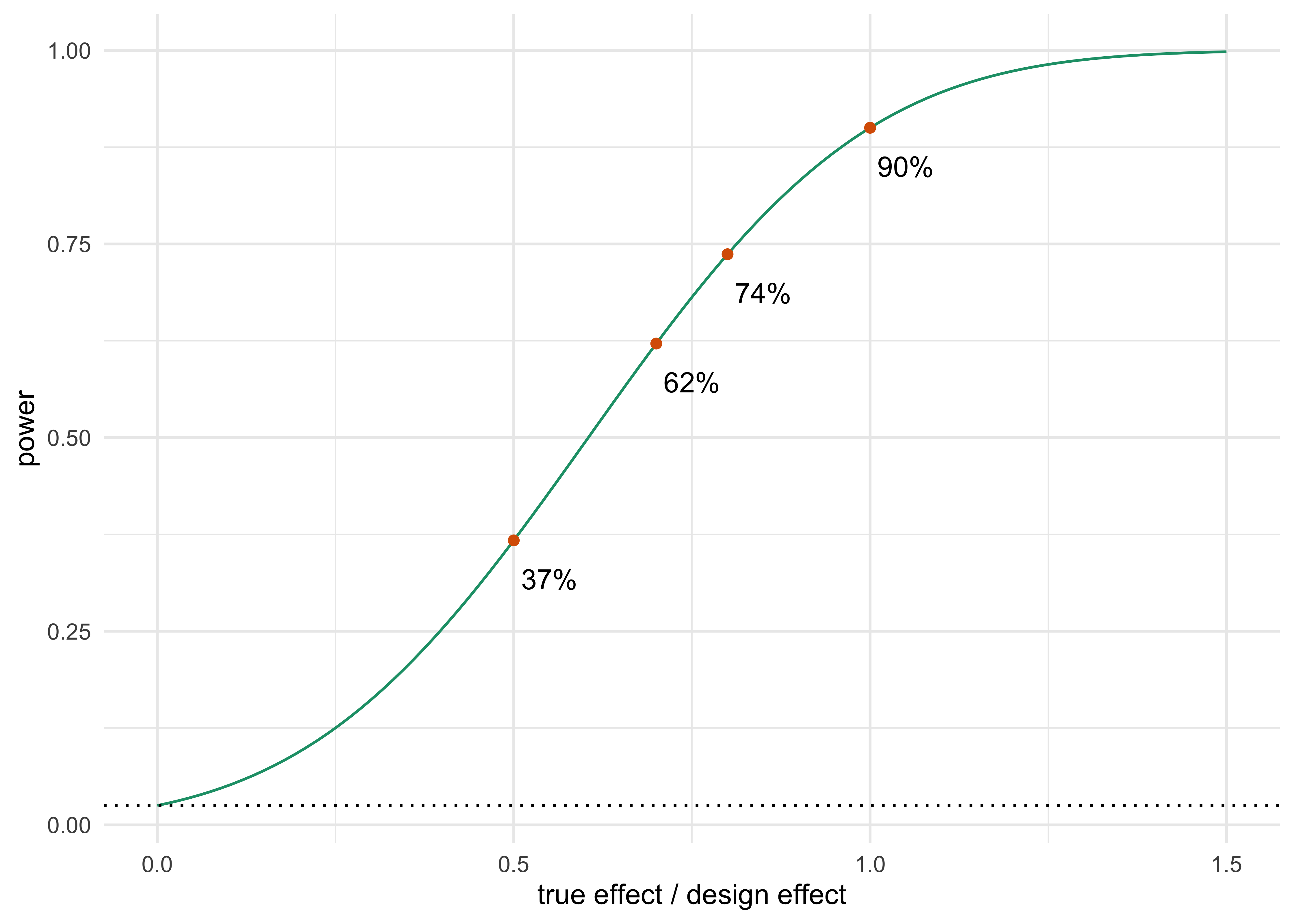
ICH E9 asks sponsors to consider how sensitive the sample size is to the assumptions. The square law makes that sensitivity easy to quantify. If the trial is sized for an effect \(\theta_d\) but the truth is \(\theta = \rho\,\theta_d\), power is \(\Phi(\rho(z_\alpha+z_\beta) - z_\alpha)\). This depends only on the ratio \(\rho\) and not on \(\theta_d\) or \(n\).

zs <- qnorm(0.975) + qnorm(0.90)
f <- function(r) pnorm(r * zs - qnorm(0.975))
pts <- data.frame(r = c(0.5, 0.7, 0.8, 1.0), p = f(c(0.5, 0.7, 0.8, 1.0)))
ggplot(data.frame(r = c(0, 1.5)), aes(r)) + stat_function(fun = f, colour = "#1B9E77") +
  geom_point(data = pts, aes(r, p), colour = "#D95F02") +
  geom_text(data = pts, aes(r, p, label = scales::percent(p, 1)), nudge_x = 0.05, nudge_y = -0.05) +
  geom_hline(yintercept = 0.025, linetype = 3) + labs(x = "true effect / design effect", y = "power") + theme_minimal()

Figure 9.1: Power of a trial sized for 90% power (one-sided 0.025) when the true effect is a fraction of the design alternative. A true effect of 70% of the design value leaves a power of about 62%.

A trial sized for 90% power has 83% power if the true effect is 90% of the design alternative, 62% power at 70% of it, and 37% at half. The converse is equally striking and less discussed: if the drug is better than assumed, the trial is overpowered and ends later than it needed to. Both errors are expensive, and the traditional design has no means of correcting either once the first patient is enrolled, other than the sample size re-estimation and interim analyses of Chapter 11.

The next table varies the design alternative over a range typical of a standardized effect and gives the information requirement, which the moderate deviation section below uses again.

th <- c(0.05, 0.10, 0.15, 0.20, 0.30, 0.50)
knitr::kable(data.frame(theta = th, n = round(n_fixed(th))), col.names = c("Design effect", "Information required"), align = "rr")

Table 9.2: Textbook information requirement \(n = 10.51/\theta^2\) at one-sided 0.025 and 90% power, for a range of design alternatives.

Design effect	Information required
0.05	4203
0.10	1051
0.15	467
0.20	263
0.30	117
0.50	42

A halving of \(\theta\) from 0.20 to 0.10 takes the requirement from 263 to 1,051. A statistician who is asked “what effect should I design for” has an unusually consequential question on her hands, and E9 section 3.5 names two ways to answer it: the smallest effect that would be clinically relevant, or the effect the sponsor anticipates. Those are different numbers. A design for the minimal clinically important difference is conservative: it gives the trial the chosen power to detect superiority when the true effect equals that minimum. It does not establish that the effect exceeds the minimum, because the null being tested is still an effect of zero, and demonstrating benefit beyond a minimum requires a different success criterion. A design for the anticipated effect is optimistic and, if the anticipation is wrong, produces a failed trial. In practice the sponsor picks something between, informed by phase 2, and that act of picking is a prior elicitation that the protocol never calls by that name. The price of getting it wrong is concrete: pivotal trials are expensive, and cost rises steeply with patients (Section 9.6.1).

The power curve

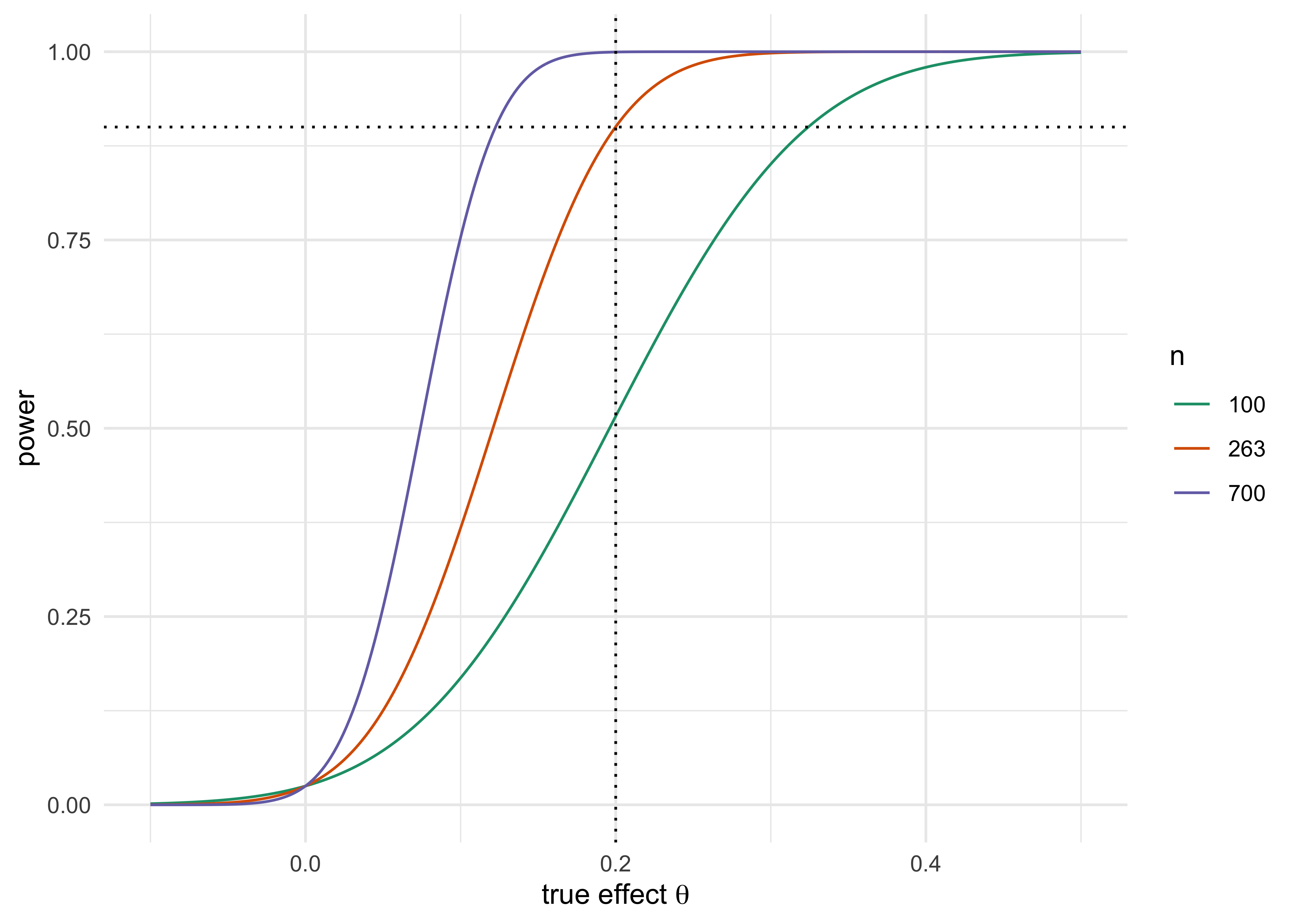
A single power number hides the shape. The power curve plots \(\text{Power}(\theta)\) for fixed \(n\) and \(\alpha\) over the whole range of effects. It equals \(\alpha\) at \(\theta = 0\), rises through 50% at \(\theta = z_\alpha/\sqrt{nI}\) and passes the design value \(\theta_d\) at \(1-\beta\).

th <- seq(-0.1, 0.5, length.out = 300); ns <- c(100, 263, 700)
d <- do.call(rbind, lapply(ns, function(n) data.frame(theta = th, power = power_z(th, n), n = factor(n))))
ggplot(d, aes(theta, power, colour = n)) + geom_line() + scale_colour_brewer(palette = "Dark2") +
  geom_vline(xintercept = 0.2, linetype = 3) + geom_hline(yintercept = 0.9, linetype = 3) +
  labs(x = expression("true effect " * theta), y = "power") + theme_minimal()

Figure 9.2: Power curves for fixed sample sizes at one-sided 0.025, with information \(nI\) of 100, 263 and 700. The middle curve is the design for \(\theta = 0.20\) at 90% power.

Two things the curve shows that a single number does not. The trial has a threshold effect, the value at which power is 50%, and effects below it are more likely to be missed than found. That value is \(z_\alpha\sqrt{1/(nI)}\), which for a design with 90% power at \(\theta_d\) is \(z_\alpha/(z_\alpha+z_\beta) = 60.5\%\) of the design effect: a trial with 90% power at a hazard ratio of 0.80 is, for an effect smaller than about a 13% hazard reduction, more likely than not to fail. And the curve is flat near the design point. Moving from 90% to 95% power at the design effect needs 24% more information, so the last points of power are bought at a steep price.

One more observation concerns the left end of the curve. The probability that the trial reports a positive result for a drug that does nothing is \(\alpha\). It does not depend on \(n\). The protocol writer who increases the sample size buys power and nothing else; the type I error stays at 0.025 however large the trial, even if a trial of 20,000 patients would, for the same observed data, support a much more skeptical conclusion than a trial of 200. The moderate deviation analysis below challenges exactly this.

What the regulator sees, and what the sponsor can do wrong

An E9 section 3.5 justification, as a regulator reads it, has five parts: the primary endpoint and estimand; the effect assumed and its source; the variability or event rate and its source; the error rates; and a sensitivity analysis. The common failures are well known to reviewers. The assumed effect is the observed effect from a small phase 2 trial, which is biased upward by selection (the drug was taken forward because it looked good). The variability is taken from the same small trial, with the uncertainty ignored. The assumed control event rate is taken from a historical cohort that no longer resembles the enrolled population. And the sponsor presents no sensitivity at all. The traditional calculation is correct as arithmetic. Its weakness is that it treats the inputs as known.

One legitimate source of a smaller required sample is a prespecified covariate-adjusted analysis: a baseline covariate that explains a fraction \(R^2\) of the outcome variance lowers the required \(n\) by about the factor \(1 - R^2\), as worked in Section 5.10, and the sample size paragraph should say whether the calculation assumes the adjusted or the unadjusted analysis.

TipIn the protocol

A sample size paragraph that survives review names: the estimand and primary analysis; the design alternative and its provenance (minimal clinically important effect or anticipated effect, with the source study); the nuisance parameters (standard deviation, control rate, event rate) with their sources; \(\alpha\) one-sided and \(1-\beta\); the resulting \(n\) or number of events and the accrual and follow-up assumptions that deliver it; and a table of power for effects at 70%, 80%, 100% and 120% of the design alternative, together with the rule for what the trial does if the nuisance parameters turn out wrong (blinded re-estimation, in an adaptive protocol under E20).

9.2 A conventional power calculation is assurance under a point-mass prior

Power is conditional

Power is a conditional probability: it is the probability of a significant result given that the true effect equals \(\theta_d\). The sponsor, the investors and the DMC are not conditioning on the truth. They want to know the probability that the trial succeeds, taking into account that they do not know the effect. A statement such as “90% power” is regularly heard in the boardroom as “90% chance of success”, which is a different claim. It would be the same claim only if the sponsor were certain that the effect equals the design value.

The traditional literature responds to this by sensitivity analysis, as above. The Bayesian response is to make the uncertainty explicit and average. Let \(\pi(\theta)\) be a prior distribution over the effect, representing everything known before the trial, such as phase 2 results, mechanism and class experience. The probability that the trial will be successful is the average of the power curve under that prior,

\[ \text{Assurance} = \int \text{Power}(\theta)\,\pi(\theta)\,d\theta . \tag{9.6}\]

O’Hagan, Stevens and Campbell (O’Hagan, Stevens, and Campbell 2005) named this quantity assurance, and earlier versions go back to Spiegelhalter and Freedman (Spiegelhalter and Freedman 1986) and Spiegelhalter, Freedman and Blackburn (Spiegelhalter, Freedman, and Blackburn 1986) under the name predictive power, and to Brown and colleagues (Brown et al. 1987) under the name expected power. Kunzmann and colleagues (Kunzmann et al. 2021) review the variants, including probability of success defined with a Bayesian rather than a frequentist final analysis. Chapter 15 uses the same logic at interim analyses, where the prior is updated by the data so far.

A closed form

For a normal prior \(\theta \sim N(m, s^2)\) and the z test above, with standard error \(\mathrm{se} = 1/\sqrt{nI}\) of \(\hat\theta\), the trial’s estimate is marginally normal with mean \(m\) and variance \(s^2 + \mathrm{se}^2\). The test succeeds when \(\hat\theta > z_\alpha\,\mathrm{se}\), so

\[ \text{Assurance} = \Phi\!\left(\frac{m - z_\alpha\,\mathrm{se}}{\sqrt{s^2 + \mathrm{se}^2}}\right). \tag{9.7}\]

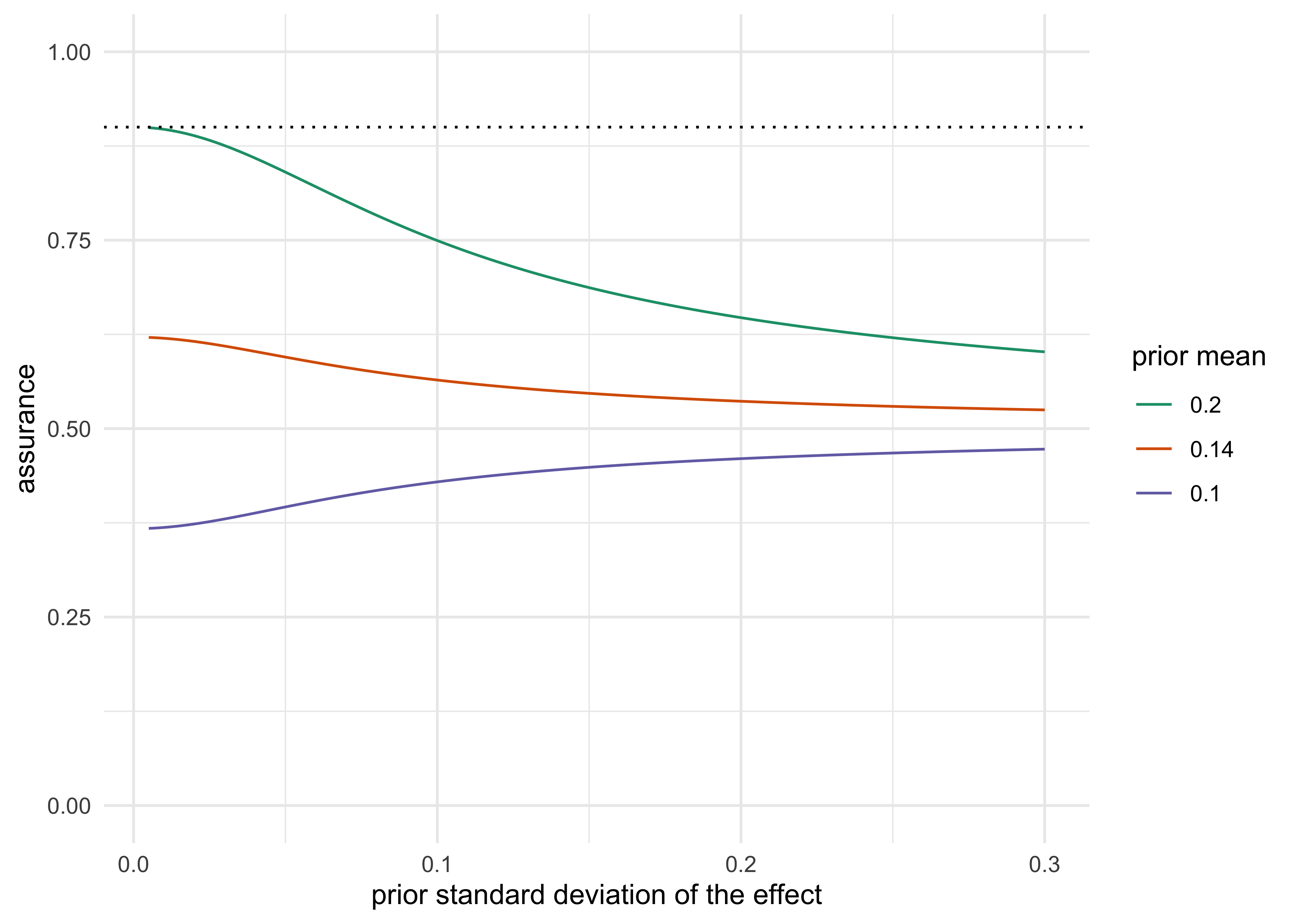
Take a trial sized for \(\theta_d = 0.20\) at 90% power (\(n = 263\), \(\mathrm{se} = 0.0617\)). Three sponsors with the same design have three beliefs. The first centers its prior at 0.20 with a standard deviation of 0.10, which is a sponsor that believes the design alternative but admits that it is uncertain by plus or minus half of itself. The second believes the drug is a bit worse, with prior mean 0.14 (70% of the design value) at the same standard deviation. The third is skeptical, with prior mean 0.10.

n <- n_fixed(0.20); se <- 1 / sqrt(n); sds <- c(0.02, 0.05, 0.10, 0.20)
tab <- sapply(sds, function(s) assurance(c(1, .7, .5) * 0.20, s, se))
knitr::kable(data.frame(c(1, .7, .5) * 0.20, tab), digits = 3, col.names = c("Prior mean", paste("SD", sds)), align = "r")

Table 9.3: Assurance of a trial sized for theta = 0.20 at 90% power, for three priors and several prior standard deviations.

Prior mean	SD 0.02	SD 0.05	SD 0.1	SD 0.2
0.20	0.889	0.840	0.750	0.647
0.14	0.616	0.595	0.564	0.536
0.10	0.373	0.396	0.429	0.460

Several things stand out in this table. With a point-mass prior (standard deviation 0.02 is close to a point) at the design value the assurance is about 0.89, near the 90% power the trial was sized for. As the sponsor becomes uncertain, assurance falls: at standard deviation 0.10 it is 0.75, and at 0.20 it is 0.65. This is not a flaw but a property of averaging. The power curve flattens as it approaches one, so the effects below \(\theta_d\) lose more power than the effects above gain. Uncertainty about the effect, even when it is symmetric around the design value, reduces the probability of success. And a skeptical sponsor, whose prior mean is 0.10 or 0.14, sees a probability of success of 43% to 56% for the very same design, although the protocol says 90%. This is not a thought experiment: when chemotherapy regimens were taken unchanged from phase II into phase III, only 28% of the phase III trials were positive (Zia et al. 2005) (see Section 9.6.3).

The “90% power” in the protocol is a statement conditional on one value of \(\theta\), and the assurance is the unconditional version. For a phase 3 trial with a program-level decision pending, assurance is the better planning quantity, and it can be computed in a spreadsheet. Spiegelhalter and Freedman’s argument, which is recognizable from the earliest days of Bayesian trial design, is that the traditional power calculation is already Bayesian in its inputs: the sponsor’s choice of \(\theta_d\) summarizes belief, but it summarizes it as a point mass and discards the uncertainty.

sd <- seq(0.005, 0.30, length.out = 200)
d <- do.call(rbind, lapply(c(1, .7, .5), function(k) data.frame(sd = sd, assurance = assurance(k * 0.20, sd, se), mean = factor(k * 0.20))))
ggplot(d, aes(sd, assurance, colour = mean)) + geom_line() + scale_colour_brewer(palette = "Dark2", name = "prior mean") +
  geom_hline(yintercept = 0.9, linetype = 3) + ylim(0, 1) + labs(x = "prior standard deviation of the effect") + theme_minimal()

Figure 9.3: Assurance of a trial sized for a design effect of 0.20 at 90% power as a function of the prior standard deviation, for three prior means. Assurance approaches the power at the design value only when the prior is concentrated on it.

What assurance is not

Assurance is not a measure of evidence. It is a forecast, computed before the data, of the frequency with which a trial of this size will cross its pre-specified threshold. The threshold is still the frequentist one in the classical version above: \(z > z_\alpha\) with \(\alpha\) fixed at 0.025. A fully Bayesian version computes the probability that the posterior probability of benefit exceeds the threshold \(c\) in the FDA draft’s criterion \(\Pr(\delta > a \mid \text{data}) > c\), with the expectation taken over the design prior. This is sometimes called Bayesian assurance, and it separates the roles of two priors. The design prior (also called the sampling prior) describes what the sponsor believes about the effect and is used to forecast. The analysis prior is the one used in the final analysis, and it is the one that has to be pre-specified and defended to the regulator (Chapter 8). A sponsor can be optimistic in the design prior and skeptical in the analysis prior; there is no inconsistency, and indeed that combination is a sound one. What the regulator will not accept is calibration of the Type I error under the design prior. Type I error is computed under the null, whatever the sponsor believes.

The FDA draft (U.S. Food and Drug Administration 2026) describes three routes (calibration, direct posterior, decision-theoretic), and this book’s default is calibration. Under the calibration route the operating characteristics reported are the type I error under the null scenarios (calibrated, typically to 0.025 one-sided), and power or probability of success under a range of alternative scenarios, shown with Monte Carlo error. Assurance is the average of the latter over the sponsor’s own prior, and it is a legitimate additional output, but it does not replace the scenario table. The other two routes justify the design differently (a direct posterior criterion, or a decision-theoretic one), but the draft still expects operating characteristics evaluated by simulation, and the draft recommends rather than requires.

A comparison

Table 9.4: Power and assurance side by side.

	Traditional power	Assurance
Treats the effect as	a single design value \(\theta_d\)	uncertain, with prior \(\pi(\theta)\)
Answers	If the effect is \(\theta_d\), how often does the test succeed?	How often will the trial succeed, given what we believe?
Inputs	\(\alpha\), \(\beta\), \(\theta_d\), nuisance parameters	the same, plus a prior for \(\theta\) and its source
Typical value	the target, 80% or 90%	lower, often 50% to 70% for a phase 3 sized on a phase 2 estimate
Regulatory status	required justification (E9 3.5)	optional; a planning aid. The scenario table of operating characteristics is what is reported

This is how assurance is used in sponsor practice, which is where a reader will meet it. Rufibach, Burger and Abt (Rufibach, Burger, and Abt 2016) study the choice of prior for Bayesian predictive power used as a probability of success in drug development and make recommendations for its use, and Crisp and colleagues (Crisp et al. 2018) report practical experience of adopting assurance as a framework for decisions in drug development. The usual pattern is a go or no-go decision on a phase 3 program: the prior is built from the phase 2 estimate and its uncertainty, often with a discount for the optimism of a selected result, elicited from the team where the data are thin, and the assurance is reported beside the design power. In the example above, a phase 2 estimate of 0.14 with standard deviation 0.10 (a 30% discount on the design effect of 0.20) turns a 90% power trial into one with assurance 56%. A phase 3 program with that number may still be worth running, but the decision is now explicit. Two cautions. Assurance is a planning quantity: it is not an error rate and it does not replace the scenario table of operating characteristics. And it is only as good as the prior, so the elicitation record and a sensitivity analysis to the discount belong with it.

Bayesian sample size criteria

Assurance is one of several ways to turn a prior into a sample size. Inoue, Berry and Parmigiani (Inoue, Berry, and Parmigiani 2005) separate the Bayesian rules into three families and show how each relates to the power calculation. The first two are named by what they average. Most of these criteria involve two priors, the design prior that predicts the data and the analysis prior that turns the data into a posterior (Wang and Gelfand (2002) call them the sampling prior and the fitting prior), and keeping the two apart (the distinction of Chapter 8) is the point of the distinction; the exception is the known-variance length criterion below, which needs no design prior. The taxonomy and the two-prior framing used here are this book’s presentation of that literature, not a development in Inoue and colleagues. Take a two-arm trial with outcome standard deviation \(\sigma = 1\), an effect \(\theta\) with design prior \(N(0.3, 0.1^2)\) and a flat analysis prior.

The next three criteria were introduced for binomial proportions by Joseph, Wolfson, and Berger (1995) and set out for means and proportions, with mixed Bayesian and likelihood versions, by Joseph, Berger, and Bélisle (1997) and, for normal means and their differences, by Joseph and Bélisle (1997); the CRAN packages SampleSizeProportions and SampleSizeMeans implement them, and Joseph and Bélisle (2019) extend them to a community of priors held by different stakeholders, sizing the trial so that skeptics and enthusiasts alike end with a narrow enough interval.

Average length criterion (ALC). Choose \(n\) so that the posterior 95% interval has expected length at most \(\ell\). With a flat analysis prior this is the familiar \(2 \times 1.96\sqrt{2\sigma^2/n} \le \ell\), so \(n \ge 2(3.92\sigma/\ell)^2\), which is 342 per arm for \(\ell = 0.3\). It needs no design prior at all when the variance is known, and it sizes a trial for estimation, not for a decision.

Average coverage criterion (ACC) and worst outcome criterion (WOC). Fix the length \(\ell\) of the interval, centered at the analysis posterior mean, and choose \(n\) so that its coverage under the design prior (the coverage actually delivered if the design prior were true) is at least a target, either on average over the data (ACC) or in the worst case over the central region of the data that contains 90% of the prior predictive probability (a modified WOC). This is the design-prior version of the criteria; in the formulation of Joseph and colleagues the coverage is the analysis-posterior mass, which with a flat analysis prior and known variance does not depend on the data, so that ACC and WOC coincide there. At \(\ell = 0.3\) the ACC is 0.87, 0.93 and 0.97 at 200, 300 and 400 per arm, and the WOC is lower, 0.68, 0.85 and 0.92, because it protects against the unlucky data and not the typical ones. When design and analysis priors coincide and the variance is known the two criteria agree.

Posterior probability criterion. Choose \(n\) so that the preposterior probability of a convincing posterior, \(\Pr\{\Pr(\theta > 0 \mid X) > 0.975\}\), reaches a target such as 0.8. With the design prior above and a flat analysis prior this is the assurance of the previous section, and it is 0.77, 0.86 and 0.91 at 200, 300 and 400 per arm. It first reaches 0.8 at 226 per arm. If the same informative prior is also the analysis prior, the probability is above 0.99 already at 50 per arm, because the prior alone gives \(\Pr(\theta > 0) = \Phi(3) = 0.9987\). The trial is then unnecessary for an analyst who holds that prior, which is the right conclusion for her and a warning against letting a sponsor’s design prior into a regulator’s analysis.

The result that ties this to the first half of the chapter is that the power calculation is the posterior probability criterion with a point-mass design prior at the alternative and a flat analysis prior (Inoue, Berry, and Parmigiani 2005). A power calculation is a Bayesian sample size calculation with an unusually confident design prior. At \(\theta = 0.3\) a two-arm trial needs 234 per arm for 90% power (the criterion evaluates to 0.90 at that size), while the assurance at 234 per arm, which acknowledges the uncertainty about \(\theta\), is 0.81. A decision-theoretic criterion, which chooses \(n\) to maximize expected utility net of the cost of sampling, is the third family; it is the one that asks how much information is worth buying, and it is the subject of Section 9.5.

The Bayesian sample size literature is wider than these families. Adcock (Adcock 1988, 1997) gave early average-criterion treatments and a review of the field, Lindley (Lindley 1997) set out the decision-theoretic choice of sample size, and Chaloner and Verdinelli (Chaloner and Verdinelli 1995) review Bayesian experimental design more generally. Wang and Gelfand (Wang and Gelfand 2002) made the simulation-based version practical. De Santis (De Santis 2006) asks for sample sizes that remain adequate across a class of priors, and Brutti and De Santis (Brutti and De Santis 2008) extend this to avoiding a range of equivalence. Gittins and Pezeshk (Gittins and Pezeshk 2000) and Sahu and Smith (Sahu and Smith 2006) mix Bayesian planning with a frequentist analysis, and Pezeshk (Pezeshk 2003) reviews the field. Read by the question each answers, the coverage and length criteria size an estimate, the posterior probability criterion and assurance size a decision, the expected-utility criteria size a decision together with its cost, and the robust criteria protect against the choice of prior. For a confirmatory trial the regulator still asks for the operating characteristics of the final analysis, so these criteria serve planning and the calibrated error rates of Chapter 14 serve the claim.

A rare-disease example: lupus

Moore and Joseph (A. D. Moore and Joseph 1999) make the case for estimation-based sample sizes in systemic lupus erythematosus, where trials are small because patients are few and follow-up is long. Their dichotomous example is progression to dialysis over five years in lupus nephritis, 50% on standard therapy and a hoped-for 25% on a new regimen. The textbook calculation with a two-sided 5% test and 90% power needs 77 patients per arm (the paper reports 77, from the normal approximation with rounded quantiles; power.prop.test gives the same after rounding up). That is a fair answer to the question it asks. The difficulty is that a 25-point reduction is a large effect, and a drug that delivers a more modest one, say 35% against 50%, needs 227 per arm, 454 in all, which may exceed the number of eligible patients in a registry of a rare disease.

The alternative the paper recommends is to size the trial to estimate the difference to a stated accuracy. A total interval width of 0.3 (plus or minus 0.15) for a 95% interval gives 75 per arm by the frequentist formula, which is the paper’s 75. Its Bayesian counterparts take a Beta prior on each proportion, here worth four prior patients per arm and centered on the design values, and ask for the same width on average (ALC), with average coverage of 95% (ACC), or with coverage of at least 95% for every possible dataset (WOC; restricting the guarantee to the central 90% of the prior predictive distribution, as in the previous section, gives the modified WOC). They were computed with Joseph and Bélisle’s package SampleSizeProportions (Joseph, Bélisle, and du Berger 2023), and the ACC is a Monte Carlo estimate with a fixed seed. The paper only mentions the Bayesian route and gives no Bayesian sample sizes, so these numbers have no published counterpart. They are smaller than the frequentist width calculation for the ALC and ACC, 55 and 57 per arm, for two reasons: the prior contributes a few patients’ worth of information, and the design prior averages \(p(1-p)\) over its support, which is below the value \(0.25\) that the plug-in formula uses at \(p = 0.5\). The WOC, 81, is larger than the plug-in answer because it protects against unlucky data. The width is also the lever that matters: widening it to 0.4 (plus or minus 0.2) cuts the Bayesian sizes to 33, 33 and 43 per arm for the modest scenario (Table 9.5).

knitr::kable(lp_tab, col.names = c("Method", "Large effect", "Modest effect"), align = "lrr")

Table 9.5: Patients per arm for a two-arm trial with a binary outcome (50% on control). The large-effect column is the lupus nephritis example of Moore and Joseph (25% on treatment, interval width 0.3); the modest-effect column is 35% on treatment with interval width 0.4. Bayesian criteria use Beta priors worth four patients per arm centered on the design proportions, and a 95% interval.

Method	Large effect	Modest effect
Power, 90% at 5% two-sided	77	227
Interval width, frequentist	75	46
Bayesian ALC	55	33
Bayesian ACC	57	33
Bayesian WOC	81	43

What the smaller trial buys and costs is the point. It buys feasibility: a trial of 66 patients in all can be run where one of 454 cannot. It costs the guarantee of a decision. At that size the trial estimates the difference to within plus or minus 0.2, so if the true effect is 15 points the interval will often include zero, and the trial is underpowered for a test of no difference. It is not underpowered for the question it was sized to answer, how large the benefit is, and an interval of that width, read with the prior in hand, is the evidence a small trial can honestly offer. The criteria also take their inputs from the design prior, so the sensitivity analysis recommended for the power calculation applies to them in the same way.

9.3 The moderate deviation sample size

The fixed-n test has no memory of n

In the textbook calculation the critical value \(z_\alpha\) is fixed. A trial of 200 patients and a trial of 20,000 patients both declare success at \(Z > 1.96\). The consequences are known to every reader who has met a very large trial that reports a result with \(p = 0.04\) and a clinically trivial effect. A statistically significant result in a huge trial is weak evidence against the null when measured the Bayesian way: the Bayes factor in favor of the alternative at \(Z = 1.96\) shrinks as the sample size grows, which is Lindley’s paradox (Chapter 7). A Bayesian decision maker who places a prior mass on the null and balances the costs of the two errors will use a critical value that increases with \(n\).

Polson and Sokolov (Polson and Sokolov 2026a), building on a result for the Bayes risk of a regular testing problem (Polson and Sokolov 2026b), work out how fast. The Bayes-optimal boundary on the standardized scale is

\[ t_{\text{crit}} = \sqrt{\log n + C}\,\bigl(1 + o(1)\bigr), \qquad C = 2\log\frac{\pi_0/\pi_a}{\pi(\theta_0)\sqrt{2\pi/I(\theta_0)}}, \tag{9.8}\]

where \(\pi_0\) and \(\pi_a\) are the prior probabilities of the null and the alternative and \(\pi(\theta_0)\) is the prior density of the effect at the null. For a unit-information prior the denominator is one and \(C = 2\log(\pi_0/\pi_a)\); with equal prior odds \(C = 0\) and the boundary is \(\sqrt{\log n}\). This is called the moderate deviation scale because the boundary grows with \(n\): it lies above the fixed value \(z_\alpha\) of the central limit regime and below the large-information approximation to the anytime-valid (large deviation) bar of the normal-mixture construction, \(\sqrt{\log n + C + 2\log(1/\alpha)}\) (an approximation for that construction, not a universal cost of anytime validity), and Chapter 11 sets the three scales side by side.

NoteTechnical note: where the boundary comes from

The Bayes rule rejects the null when the posterior probability of the alternative exceeds one half, after weighting by the prior probabilities. Compare the two marginal likelihoods. Under the null, the standardized statistic has the standard normal density \(\phi(t)\). Under the alternative, with a prior \(\pi\) smooth at \(\theta_0\), the marginal density of the data is, by Laplace’s method, proportional to \(\pi(\theta_0)/\sqrt{nI(\theta_0)}\), because the prior mass that is compatible with the data has width of order \(1/\sqrt{nI}\). The balance condition is

\[ \pi_0\,\phi(t_n) = \pi_a\,\frac{\pi(\theta_0)}{\sqrt{n\,I(\theta_0)}}, \]

which equates a Gaussian density to an \(n^{-1/2}\) term. Taking logarithms, \(t_n^2/2 = \tfrac12\log n + \text{constant}\), hence \(t_n^2 = \log n + C\). The constant collects the prior odds and the prior density at the null. For a standard Cauchy prior on a unit-variance Gaussian mean the asymptotic approximation is \(t_{\text{crit}} = \sqrt{\log(\pi n/2)}\), which is \(C = \log(\pi/2) = 0.452\). The expression holds asymptotically; it is an approximation in \(n\) and the \(o(1)\) matters at small sample sizes.

Two quick numbers fix ideas. The boundary with \(C = 0\) exceeds the textbook 1.96 for every \(n\) above 46 (since \(\sqrt{\log 46} = 1.96\)). At \(n = 1000\) it is 2.63 and at \(n = 10{,}000\) it is 3.03. The induced type I error, which is no longer fixed, is exactly \(1-\Phi(t)\) one-sided and twice that two-sided; the Mills-ratio approximation \(2\phi(t)/t\) for the two-sided value is accurate only for large \(t\), and the error falls like \((n\log n)^{-1/2}\). This chapter reports the exact one-sided value, to match the one-sided 0.025 of the textbook design.

The power function and the sample size equation

The power of the moderate deviation rule against an effect \(\theta\) follows by the same normal approximation as before, with the fixed \(z_\alpha\) replaced by the boundary:

\[ \text{Power}_n(\theta) = \Phi\!\left(\sqrt{nI}\,\theta - \sqrt{\log n + C}\right) + o(1), \qquad \theta > 0 \text{ for the one-sided benefit rule}. \tag{9.9}\]

Setting this equal to \(1-\beta\) gives the sample size equation

\[ n\,I\,\theta^2 = \left(\sqrt{\log n + C} + z_\beta\right)^2 . \tag{9.10}\]

Set it beside Equation 9.2. The structure is identical, but \(z_\alpha\) has been replaced by \(\sqrt{\log n + C}\), a quantity that depends on \(n\) itself. The equation is implicit, but only through a logarithm, and a fixed-point iteration converges in a handful of steps: compute the textbook \(n\), put it into \(\sqrt{\log n + C}\), recompute, and repeat. In the code the equation is solved with a root finder.

zb <- qnorm(0.90); n <- (qnorm(0.975) + zb)^2 / 0.2^2; it <- n
for (k in 1:4) { n <- (sqrt(log(n)) + zb)^2 / 0.2^2; it <- c(it, n) }
knitr::kable(data.frame(0:4, it), digits = 1, col.names = c("Iteration", "Information"), align = "rr")

Table 9.6: Fixed-point iteration for the moderate deviation sample size at theta = 0.20, C = 0, 90% power, starting from the textbook answer with z = 1.96 (two-sided 5%, the convention of POL’s tables).

Iteration	Information
0	262.7
1	331.6
2	340.5
3	341.5
4	341.7

The iterates are 262.7, 331.6, 340.5, 341.5 and 341.7, and the exact root is 341.7, which agrees with the values reported by Polson and Sokolov.

A note on units, since the tables can otherwise confuse. In Equation 9.10 the quantity \(n\) is the sample size on the scale where one unit carries information \(I\), so that \(nI\) is the total information. For a one-sample or paired standardized mean difference with \(I = 1\), \(n\) is the number of patients. For a two-arm trial with 1:1 allocation and a standardized effect, the information is \(N/4\), so the number of patients is \(N = 4n\). For a logrank test there are two equivalent conventions: count in events with \(n = d\) and \(I = 1/4\), or count in information units with \(n = d/4\) and \(I = 1\). The boundary \(\log n + C\) must describe the same rule in both, so the constant moves with the unit: \(\log(d/4) + C_{\text{info}} = \log d + C_{\text{events}}\), that is \(C_{\text{info}} = C_{\text{events}} + \log 4\). Keeping \(C = 0\) while switching units changes the implied prior. The package function events_md() uses the information convention (\(n = d/4\), \(I = 1\)), so its \(C = 0\) is the unit-information prior at equal prior odds on that scale, and \(C = 2\log(\pi_0/\pi_a)\) holds in that convention. The same numerical \(C = 0\) read in the events convention means \(C_{\text{info}} = \log 4 = 1.39\), the constant of two-to-one odds in the information convention, and at a hazard ratio of 0.80 it calls for 1255 events rather than 1067. Any stated value of \(C\) must therefore name its unit. All tables below use the information convention, and the comparison with the textbook formula is made in the same units.

The surprising result

Table 9.7 compares the textbook information requirement with the moderate deviation requirement. The textbook column uses the two-sided 5% convention, \(z = 1.96\), because that is the convention of the comparison in POL; at one-sided 0.025 the critical value is the same.

th <- c(0.05, 0.10, 0.15, 0.20, 0.30, 0.50); nt <- n_fixed(th); nm <- n_md(th); tb <- sqrt(log(nm))
knitr::kable(data.frame(th, round(nt), round(nm), round(nm / nt, 2), tb, pnorm(-tb)), digits = c(2, 0, 0, 2, 3, 5), col.names = c("Design effect", "Textbook", "Moderate deviation", "Ratio", "Boundary", "Type I error (one-sided)"), align = "r")

Table 9.7: Information required for 90% power, textbook versus moderate deviation (C = 0, information convention). The last two columns are the boundary at the moderate deviation sample size and the exact one-sided type I error it induces, 1 - Phi(boundary).

Design effect	Textbook	Moderate deviation	Ratio	Boundary	Type I error (one-sided)
0.05	4203	7271	1.73	2.982	0.00143
0.10	1051	1598	1.52	2.716	0.00330
0.15	467	651	1.39	2.545	0.00546
0.20	263	342	1.30	2.415	0.00786
0.30	117	136	1.16	2.216	0.01333
0.50	42	41	0.98	1.928	0.02690

The moderate deviation design needs more, not fewer, patients than the nominal textbook calculation for every effect smaller than about 0.5. At \(\theta = 0.20\) the ratio is 1.30, so the moderate deviation fixed design is about 30% larger; at \(\theta = 0.10\) it is 1.52 and at \(\theta = 0.05\) it is 1.73. Only for large effects, at which the requirement is below 46 units and the boundary is below 1.96, does the ordering reverse.

The reason is that the Bayes boundary is more demanding than 1.96 for any trial of moderate or large size: a test that demands \(Z > 2.42\) rather than \(Z > 1.96\) needs more information to reach 90% power.

What the extra patients buy is in the last column. The one-sided type I error is no longer held at 2.5% at all sample sizes but falls as \(n\) grows: 0.79% at \(\theta = 0.20\) (the two-sided equivalent is twice that), 0.33% at \(\theta = 0.10\) and 0.14% at \(\theta = 0.05\). At a thousand units of information the induced one-sided error is 0.43% and at ten thousand 0.12%. POL’s reading is that a fixed error is the right error for no sample size in particular. Whether one accepts that reading or not, the arithmetic is clear: a design that maintains a lower error as information accumulates cannot be cheaper than one that does not.

The prior odds in the constant

The constant \(C\) makes the dependence on prior belief explicit. With the unit-information prior, \(C = 2\log(\pi_0/\pi_a)\), and moving from even odds to two-to-one and four-to-one against the alternative raises \(C\) from 0 to 1.39 and 2.77.

o <- c(1, 2, 4); C <- 2 * log(o); nm <- n_md(0.20, C); tb <- sqrt(log(nm) + C)
knitr::kable(data.frame(o, C, round(nm), tb, pnorm(-tb)), digits = c(0, 2, 0, 3, 5), col.names = c("Odds against", "C", "Information", "Boundary", "Type I error (one-sided)"), align = "r")

Table 9.8: Effect of prior odds (null to alternative) on the moderate deviation requirement at theta = 0.20, 90% power, information convention. Type I error is the exact one-sided value.

Odds against	C	Information	Boundary	Type I error (one-sided)
1	0.00	342	2.415	0.00786
2	1.39	400	2.716	0.00330
4	2.77	454	2.982	0.00143

The requirement rises from 342 to 400 and 454 information units, and the induced one-sided error falls from 0.79% to 0.33% and 0.14%. Skepticism is paid for in patients, at a rate the formula makes explicit. This is the property a protocol reviewer wants: the sponsor who claims the drug is a long shot is told how many more patients it will take, and the sponsor who claims equal prior odds is told what that claim is worth.

It also shows what this approach does not do. It is not a method of getting out of a regulatory error-rate expectation. Where the sponsor takes the FDA draft’s calibration route, with a one-sided type I error of 0.025 verified by simulation, that target stays; the moderate deviation analysis is a design-stage theory of why a trial of a given size should be held to a stricter standard than the nominal one, and of the cost of holding it there.

Many parameters and many endpoints

Two extensions carry over into design (Polson and Sokolov 2026b). For a \(d\)-dimensional parameter, for instance a trial with \(d+1\) arms, the boundary is \(\sqrt{d\log n}\), so at \(n = 1000\) the radius is 2.63 for one parameter, 3.72 for two and 4.55 for three. This is the moderate deviation form of the Schwarz penalty \(d\log n\), a Bayesian counterpart of a multiplicity correction arrived at without reference to a family of tests (Chapter 10). Both extensions are model-based approximations (a regular parametric model with \(d\) free parameters for the first, sparsity of the true signals for the second), and neither displayed expression by itself controls the familywise error rate across clinical claims. For \(p\) simultaneous endpoints or subgroups under sparsity the boundary is the universal threshold \(\sqrt{2\log p}\), which is 3.03 at a hundred endpoints and 4.45 at twenty thousand, the latter being the scale of a genome-wide scan.

knitr::kable(rbind(data.frame(case = paste("d =", 1:3, ", n = 1000"), boundary = sqrt((1:3) * log(1000))),
      data.frame(case = paste("p =", c(100, 2000, 20000)), boundary = sqrt(2 * log(c(100, 2000, 20000))))),
      digits = 2, col.names = c("Case", "Boundary"), align = "lr")

Table 9.9: Boundaries for d parameters at n = 1000, and for p endpoints under sparsity.

Case	Boundary
d = 1 , n = 1000	2.63
d = 2 , n = 1000	3.72
d = 3 , n = 1000	4.55
p = 100	3.03
p = 2000	3.90
p = 20000	4.45

Reading SELECT against the formulas

SELECT is the natural trial against which to read these formulas, with a caution stated first: it does not test the moderate deviation theory. SELECT was designed for a hazard ratio of 0.83 (a 17% reduction), with 90% power, one-sided 0.025, 1,225 planned events and one superiority interim analysis at two thirds of the planned events, followed by the final analysis (Ryan et al. 2020). The observed hazard ratio was 0.80 on 1,270 events (Lincoff et al. 2023) (Chapter 21 gives the trial in detail). The design hazard ratio, not the observed one, is the design alternative, and the table sets both beside each calculation.

options(knitr.kable.NA = "")
knitr::kable(data.frame(calculation = c("textbook, HR 0.83 (design)", paste0("moderate deviation, HR 0.83, ", c(1, 2, 4), ":1 odds"),
                                        "textbook, HR 0.80 (observed)", paste0("moderate deviation, HR 0.80, ", c(1, 2, 4), ":1 odds"),
                                        "SELECT as planned", "SELECT as observed"),
           events = round(c(ev83, md83["events", ], ev80, md80["events", ], 1225, 1270)),
           t_crit = round(c(qnorm(0.975), md83["t", ], qnorm(0.975), md80["t", ], NA, NA), 2)),
  col.names = c("Calculation", "Events", "Critical value"), align = "lrr")

Table 9.10: Events for 90% power: textbook against moderate deviation (information convention), at the design hazard ratio 0.83 and at the retrospective hazard ratio 0.80, with the events planned and observed in SELECT.

Calculation	Events	Critical value
textbook, HR 0.83 (design)	1211	1.96
moderate deviation, HR 0.83, 1:1 odds	1603	2.45
moderate deviation, HR 0.83, 2:1 odds	1867	2.74
moderate deviation, HR 0.83, 4:1 odds	2119	3.01
textbook, HR 0.80 (observed)	844	1.96
moderate deviation, HR 0.80, 1:1 odds	1067	2.36
moderate deviation, HR 0.80, 2:1 odds	1255	2.67
moderate deviation, HR 0.80, 4:1 odds	1433	2.94
SELECT as planned	1225
SELECT as observed	1270

At the design hazard ratio of 0.83 the textbook formula gives 1211 events against the 1,225 planned, a difference of 14 events, about 1% of the plan. There is nothing substantial left over for a moderate deviation standard to explain. The moderate deviation formula at the same hazard ratio and equal prior odds gives 1603 events, far above the plan, so it does not predict SELECT’s size. The textbook 844 events at the observed 0.80 is a retrospective number and was never SELECT’s design target.

The moderate deviation sample-size theory stands on its own terms and does not need SELECT. It says what a fixed design would cost if the type I error were allowed to fall with information, and what the prior odds in \(C\) are worth in patients. Whether sponsors and regulators in practice demand that kind of stricter standard from very large trials is an empirical question for many trials, and one trial whose size is explained by its own stated design assumptions does not answer it. A protocol’s event target also reflects considerations that no formula captures: safety database size, subgroup precision, competing events and secondary endpoints.

Where the saving is, and where it is not

A fixed-sample Bayesian design using the uncalibrated moderate deviation boundary is larger than the nominal textbook design, by about 30% at \(\theta = 0.20\), and it buys a type I error that falls with \(n\). The Bayesian saving in patients and time does not come from the fixed design at all. Against a single unadjusted analysis at a fixed sample size, the calibrated Bayesian bar is never lower without an informative prior, and the uncalibrated Bayes boundary is higher once the information \(q = n\tau^2\) exceeds 41.6 (that is, \(n > 41.6\) in the unit-information case); that is the thesis of this book and this chapter is its arithmetical base. The saving comes from monitoring. Once the trial is allowed to stop when the posterior is decisive, the same boundary that was expensive to reach at the design stage is reached early along most trajectories. In the SELECT reconstruction of Chapter 12 (a counterfactual with true hazard ratio 0.80 and at most 1,270 events), among simulated trials that declare efficacy the median stopping point is 464 events for a calibrated Bayesian monitoring rule (power 0.95), 612 for an e-value rule (power 0.83) and 952 for a four-look O’Brien-Fleming design (power 0.98), against 817 for SELECT’s planned two-look design (power 0.97); Table 12.2 gives the medians over all trials, the realized type I errors and the conditioning. The same arithmetic, applied to whole programs rather than single trials, is the platform-trial claim of Saville and Berry (Saville and Berry 2016) (see Section 9.6.4 and Chapter 20). A sponsor who goes to the regulator with a Bayesian fixed-sample design and a claim that it is cheaper than the traditional one has made a claim that this chapter’s arithmetic contradicts.

Equally, the traditional design deserves its fair credit. If the trial will be run once, analyzed once, at a fixed time, with no interim looks, the textbook design is simpler, its operating characteristics are known in closed form, and its regulatory path is established. POL itself concedes the case of REWIND, in which a scheduled design does better (Chapter 21). A sponsor that cannot commit to a monitoring plan has no reason to move.

9.4 Side by side

Table 9.11: What changes in the protocol, and what stays. Where the two agree numerically: with a normal likelihood and a flat prior and the same one-sided threshold, \(\Pr(\theta>0\mid y) = 1-p_{\text{one-sided}}\), so the corresponding decision thresholds agree (Chapter 7).

Aspect	Traditional fixed design	Bayesian, same fixed sample	Bayesian, monitored
Sample size rule	\(n = (z_\alpha+z_\beta)^2/(I\theta^2)\)	\(nI\theta^2 = (\sqrt{\log n + C}+z_\beta)^2\), for the pure Bayes rule; the textbook \(n\) if calibrated to 0.025	maximum sample size and boundaries chosen jointly to achieve target power
Type I error	0.025 at every \(n\)	calibrated to 0.025 by choice of \(c\), or falling with \(n\) under the pure Bayes rule	calibrated to 0.025 by simulation (Chapter 14)
Required size, same power	baseline	larger (about 30% at \(\theta = 0.20\) for the pure Bayes rule)	smaller in expectation than a fixed design after matching power and error targets, because of early stopping
Design alternative	point value \(\theta_d\), implicit prior	explicit design prior, assurance	explicit design prior, predictive probability at interims
What the regulator asks	E9 3.5 justification and sensitivity	calibration and operating characteristics report (FDA draft IV.A)	the same, plus the monitoring plan and simulation report (E20, FDA adaptive 2019)

When the Bayesian criterion is calibrated so that the familywise type I error is 0.025, which is this book’s default for confirmatory designs without borrowing and one of the routes the FDA draft describes (U.S. Food and Drug Administration 2026), the fixed-sample Bayesian and traditional designs reach the same threshold and need the same sample size for the same power, because calibration reproduces the traditional critical value in the one-look case. The difference in sample size between the “pure Bayes” boundary and the textbook arises when the error rate is allowed to fall with \(n\). That distinction is worth keeping in mind when reading claims about Bayesian sample sizes: the claim must say which of the two it refers to.

9.5 Sizing for the population

Every calculation so far takes the two error rates as given. A decision-theoretic planner has no error rates to take. Consider the problem of Anscombe (Anscombe 1963) and Colton (Colton 1963). A population of \(N\) patients will be treated over the relevant horizon. Before treating them the planner randomizes \(2n\), \(n\) to each of two treatments, with a normal outcome of known standard deviation \(\sigma\), so the difference in means is \(N(\theta, 2\sigma^2/n)\). The effect has prior \(\theta \sim N(0, \tau^2)\) (a simplifying symmetry assumption that treats the two arms as exchangeable before the trial; a planner who currently prefers one arm can still value the trial, and a nonzero prior mean would shift the optimum), and after the trial the remaining \(N - 2n\) patients receive the arm with the higher posterior mean. Welfare is linear in \(\theta\), and the cost of the trial is the welfare of its participants, half of whom receive the inferior arm. The expected loss against full information is

\[ L(n) = n\,\tau\sqrt{2/\pi} + (N - 2n)\,\frac{\tau(1 - \rho)}{\sqrt{2\pi}}, \qquad \rho = \frac{\tau}{\sqrt{\tau^2 + 2\sigma^2/n}}, \tag{9.11}\]

where the first term is the price of experimentation and the second is the price of residual ignorance. For large \(N\) the minimizer has a closed form,

\[ n^\star = \frac{\sigma}{\tau}\sqrt{\frac{N}{2}}, \qquad L(n^\star) \approx 2\sigma\sqrt{\frac{N}{\pi}}, \tag{9.12}\]

the square root rule: the optimal trial enrolls \(\sqrt{N}\)-order patients, not a multiple of \(N\). The leading-order approximation balances the experimentation and residual-ignorance terms, the usual signature of a loss of the form \(an + b/n\). The same problem was posed for clinical trials by Cornfield, Halperin and Greenhouse (Cornfield, Halperin, and Greenhouse 1969), who proposed an adaptive procedure for sequential clinical trials. It is the clinical-trial counterpart of the Anscombe and Colton problem, in which the horizon is the population that will be treated, and Chapter 16 returns to that view as the bandit problem.

sqt <- size_sqrt_table(c(1e5, 1e6), tau = 1.3, sigma = 2)
knitr::kable(data.frame(N = format(sqt$N, scientific = FALSE, big.mark = ","), n_star = round(sqt$n_star, 1), n_exact = sqt$n_opt,
  loss_exact = round(sqt$loss_min, 1), loss_approx = round(sqt$loss_approx, 1), rel_error = sprintf("%.2f%%", 100 * sqt$rel_error)),
  col.names = c("N", "n* (rule)", "n (exact)", "Loss (exact)", "Loss (rule)", "Rel. error"), align = "r")

Table 9.12: The square root rule against direct minimization of the exact loss, tau = 1.3, sigma = 2 (outcome units). Rel. error is the excess of the approximate minimum loss over the exact one.

N	n* (rule)	n (exact)	Loss (exact)	Loss (rule)	Rel. error
100,000	344.0	340	707.5	713.6	0.86%
1,000,000	1087.9	1084	2250.6	2256.8	0.27%

The rule is accurate where it is used: at \(N = 10^6\) the closed form is within 0.27% of the exact loss and at \(N = 10^5\) within 0.86%, the larger error being the \(O(1)\) correction to an \(O(\sqrt N)\) leading term. Three features matter for the contrast with practice. First, the optimal trial is small relative to the population it serves: at \(N = 10^6\) and \(\sigma/\tau = 2\) it is 1414 per arm. Second, it contains no significance level, no power and no design alternative, so one-sided 0.025 and 80% or 90% power appear as conventions and not as decision-theoretic primitives. Third, prior dispersion shrinks the optimal trial: a larger \(\tau\) makes the sign of the effect easier to learn, and a small \(\tau\) (effects known in advance to be small) makes \(n^\star\) large. Trials are large because effects are small, which is the same message as the square law of Equation 9.2 arrived at from the other end.

The planner’s rule and the regulator’s rule answer different questions. The planner sizes the trial to the population that will use the result and trades the participants’ welfare against the value of the information; the regulator asks whether this trial, by its own data, controls the probability of a false claim. They are not reconciled by a sampling cost. Adding a monetary cost per patient to Equation 9.11 changes the optimal sample size (the first-order condition becomes \(n^\star = \sigma\sqrt{N/(2\tau^2 + 2\sqrt{2\pi}\,c\,\tau)}\) for a cost \(c\) per patient in the units of \(\theta\), as size_sqrt_rule() implements), but not the terminal decision: choosing the arm with the higher posterior mean selects the experimental arm with probability one half under the null whatever \(n\) is, so the rule controls no error rate. Population welfare and regulatory success are separate criteria. A planner who also wants error control would impose a calibrated success rule as a constraint and re-optimize \(n\) under it, and the sample sizes the textbook formula produces may sit in the same flat region of the loss when the design alternative is sensible. Neither the cost nor the loss is a regulatory requirement; the first-order condition is the model’s, and Chapter 15 and Chapter 12 take the same decision-theoretic logic into monitoring.

9.6 In practice

What a sample size costs

The square law has a price list. Moore and colleagues estimated the cost of the 138 pivotal trials behind the 59 novel agents the FDA approved in 2015 and 2016 (T. J. Moore et al. 2018): a median of US$19.0 million per trial (interquartile range 12.2 to 33.1 million), a mean of US$157.2 million for the five cardiovascular trials (the costliest single trial, a noninferiority trial with clinical-benefit endpoints, was US$346.8 million), and by design a mean of US$13.5 million for trials without a control group, 28.8 million with a placebo and 48.9 million with an active comparator. A second study of 225 pivotal trials for 101 drugs approved in 2015 to 2017 (T. J. Moore et al. 2020) put the median at US$41,413 per patient (interquartile range 29,894 to 75,047), with patients per trial ranging from 4 to 8,442, and found that cost rose exponentially with patients and clinic visits (\(R^2 = 0.696\)). These are estimates assembled from public sources, not sponsor accounts, and they are medians over very different trials. The lesson for this chapter is the multiplier. A design alternative chosen 30% too optimistic does not cost 30% more when the shortfall is discovered: by the square law of Equation 9.2, a true effect of 70% of the design value needs about twice the events (1/0.49), and at the per-patient prices above a trial that must double is a nine-figure decision. The sample size sentence in the protocol is a budget line.

SELECT: sizing a cardiovascular outcomes trial

SELECT (Lincoff et al. 2023; Ryan et al. 2020) is worked through above, where the design hazard ratio, the observed one and each formula are set side by side (Table 9.10), and the trial is described in full in Chapter 21. In the language of this chapter: the sponsor designed for a more modest effect than the one it observed, and the planned size is what the textbook formula gives for that design alternative, 1211 events. The regulator did not ask for a Bayesian design, and the moderate deviation sizes are reported for comparison and do not explain the plan.

Phase II to phase III: why the design alternative is too large

The usual source of the design alternative is a phase II trial, and Zia and colleagues examined how that fares (Zia et al. 2005). Of 181 phase III studies in advanced solid tumors published from July 1998 to June 2003, 43 used regimens identical to those in 49 preceding phase II studies. Twelve of the 43 phase III studies (28%) were positive, 81% had lower response rates than the phase II study that preceded them, and the mean difference was 12.9 percentage points. The mechanism is the selection effect of the “What the regulator sees” subsection above: a drug is taken into phase III because phase II looked good. A design alternative equal to the phase II estimate is therefore biased upward, a trial sized on it is underpowered at the true effect (Figure 9.1), and the probability that it succeeds is the assurance of Table 9.3, not the 90% in the protocol. This is the case for assurance. A prior that shrinks the phase II estimate, as in the sponsors with prior mean 0.14 or 0.10 above, reports the probability of success the program will actually face, and if the answer is uncomfortable the time to learn it is before the trial is funded. The caveat is scope: the study concerns chemotherapy in solid tumors, and other areas differ.

The sponsor’s question is then not only how likely the trial is to succeed but what size maximizes the expected value of the program. Suppose, as a synthetic example, that the phase II posterior is flat, \(\theta \sim N(0.30, 0.141^2)\) on a standardized scale, and the pivotal trial randomizes \(n\) per arm and succeeds if the one-sided \(z\) statistic exceeds 1.96. Power at \(\theta\) is \(\Phi(\theta\sqrt{n/2} - 1.96)\), and the assurance averaged over a posterior \(N(m, v)\) is Equation 9.7 with \(\mathrm{se}^2 = 2/n\). Take a fixed cost of US$20 million plus US$0.1 million per patient (so \(0.2n\) for \(2n\) patients), approval after success with probability 0.9, and a value of US$1 billion for an approved drug. The expected net present value, in millions, is \(\mathrm{ENPV}(n) = 0.9 \times 1000 \times A(n) - (20 + 0.2n)\). A skeptical sponsor shrinks the same estimate to \(N(0.20, 0.115^2)\).

pf <- decide_pivotal_table(m = 0.30, v = 0.141^2); ps <- decide_pivotal_table(m = 0.20, v = 0.115^2)
of <- decide_pivotal_optimum(0.30, 0.141^2); os <- decide_pivotal_optimum(0.20, 0.115^2)
pw <- function(x) ifelse(x > 0.995, ">0.99", sprintf("%.2f", x))
knitr::kable(data.frame(pf$n, pf$cost, pw(pf$power), sprintf("%.2f", pf$assurance), round(pf$enpv), pw(ps$power), sprintf("%.2f", ps$assurance), round(ps$enpv)),
  col.names = c("n per arm", "Cost", "Power (flat)", "Assurance (flat)", "ENPV (flat)", "Power (skeptical)", "Assurance (skeptical)", "ENPV (skeptical)"), align = "r")

Table 9.13: Sizing a pivotal trial (synthetic example). Power is evaluated at the posterior mean; money in millions of US dollars. Flat posterior N(0.30, 0.141^2), skeptical posterior N(0.20, 0.115^2).

n per arm	Cost	Power (flat)	Assurance (flat)	ENPV (flat)	Power (skeptical)	Assurance (skeptical)	ENPV (skeptical)
200	60	0.85	0.73	594	0.52	0.51	399
300	80	0.96	0.80	644	0.69	0.61	470
400	100	0.99	0.85	662	0.81	0.68	508
500	120	>0.99	0.87	665	0.89	0.72	527
600	140	>0.99	0.89	661	0.93	0.75	535
800	180	>0.99	0.91	640	0.98	0.79	533
1000	220	>0.99	0.92	612	0.99	0.82	517

Two readings. First, power at the estimate overstates the chance of success: at 300 per arm the flat posterior gives power 0.96 but assurance 0.80, because the posterior puts weight on smaller effects, and under the skeptical posterior the same trial has assurance 0.61. Second, the optimum is flat and the prior moves it: the ENPV peaks near 482 per arm for the flat posterior and near 671 for the skeptical one, and both curves are within a few percent of their maximum from 400 to 800 per arm. The skeptical sponsor runs the larger trial because it needs more information to detect a smaller effect. The figures are an illustration of the arithmetic with invented costs and value, not a forecast, and the go decision is easy here because ENPV is several hundred million dollars in both columns; with a value of US$300 million the skeptical ENPV at 600 per arm falls to 63 million, still positive but thin, and the decision then depends on alternative uses of the budget.

Platform arithmetic

Saville and Berry simulated 5,000 drug-development programs under stated assumptions (200 patients enrolled per year, three months between trials) (Saville and Berry 2016). A traditional sequence of two-arm trials used 1,966 patients, had 1,357 patient failures, took 12.0 years and found an effective treatment with probability 0.78. An open adaptive platform with response-adaptive randomization and ten active arms used 640 patients, had 431 failures, took 3.2 years and had probability 0.87. That platform compares each arm with all control patients, including those enrolled before the arm entered; their concurrent-control strategy 3d used 912 patients and took 4.6 years, with success probability 0.83. It also differed in arm count, sample-size caps and efficacy threshold, so this contrast does not isolate control borrowing. These are simulations, not empirical results, but they show where the saving this chapter locates in monitoring becomes large: it compounds over a program through shared controls and early stopping. The designs and their operating characteristics are the subject of Chapter 20.

Key points

NoteKey points

• The textbook formula is \(n = (z_\alpha+z_\beta)^2/(I\theta^2)\), with \((z_\alpha+z_\beta)^2 = 10.51\) at one-sided 0.025 and 90% power and 7.85 at 80%. Binary, continuous and time-to-event endpoints differ only in what \(I\theta^2\) is: for events, \(d = 4(z_\alpha+z_\beta)^2/\log(\mathrm{HR})^2\), which gives 844 events at HR 0.80 and 90% power.
• Sample size scales as \(1/\theta^2\), so the design alternative is the most consequential and least certain input. A trial sized for 90% power has about 62% power if the true effect is 70% of the design value.
• A conventional power calculation can be represented as assurance under a point-mass design prior. The conventional calculation itself does not assert certainty about the effect or specify an analysis prior. Averaging the power curve over an explicit prior gives assurance, which is typically well below the nominal power (0.75 for a prior standard deviation of half the design effect in the worked example). Assurance is a planning forecast, not a replacement for the scenario table of operating characteristics.
• The moderate deviation sample size equation \(nI\theta^2 = (\sqrt{\log n + C} + z_\beta)^2\), with \(C = 2\log(\pi_0/\pi_a)\), replaces the fixed \(z_\alpha\) by a boundary growing like \(\sqrt{\log n}\). At \(\theta = 0.20\) it asks for 342 information units against 263, about 30% more, and it drives the type I error down with \(n\).
• The Bayesian saving is not in the fixed design. A calibrated fixed-sample Bayesian design is at best equal to the traditional one and, on the pure moderate deviation scale, larger. The saving is in monitoring, the subject of 11 and 21.
• Bayesian sample size criteria (average length, average coverage, worst outcome, posterior probability) generally depend on a design prior and an analysis prior; the known-variance average-length criterion needs no design prior. The power calculation is the posterior probability criterion with a point-mass design prior and a flat analysis prior. For a design prior \(N(0.3, 0.1^2)\), 90% power needs 234 per arm and assurance first reaches 0.8 at 226.
• A decision-theoretic planner needs no error rates: the square root rule \(n^\star = (\sigma/\tau)\sqrt{N/2}\) sizes the trial to the population it serves, and it is within 0.86% of the exact minimum loss at \(N = 10^5\). In a program, the size that maximizes expected net present value is flat and moves with the prior.
• SELECT was designed for a hazard ratio of 0.83 with 1,225 events, and the textbook formula at that design gives about 1,211. The moderate deviation formula does not predict SELECT’s size; the observed hazard ratio of 0.80 is a retrospective scenario.
• Regulators ask for the sample size justification (E9 3.5), for sensitivity to its assumptions, and, for a Bayesian design, for simulated operating characteristics, with the success criterion either calibrated to a type I error or justified by another route the January 2026 FDA draft describes.

TipTry it in the lab

Open module 03, Errors and power, go to the worked design (effect 3 points, standard deviation 10) and write down the number of patients you expect for half the effect before moving the slider; then check it, and repeat for the hazard ratio of 0.8 in the events panel.

NoteDiscussion questions

1. A sponsor sizes a phase 3 trial for 90% power at the effect observed in a 60-patient phase 2 trial. Using what you know about selection and the square law, which direction is the error in the design alternative likely to be, and how would you quantify the effect on the probability of success?
2. The protocol states 90% power and the investor reads 90% chance of success. Write the two sentences you would give the sponsor so that the board knows what the number means, and say what extra input you would need to compute the assurance.
3. The moderate deviation calculation (with \(C = 0\) in the information convention) calls for 30% more information at \(\theta = 0.20\) than the textbook formula. A regulator accepts a fixed-sample Bayesian design whose success criterion is calibrated to a type I error of 0.025. Does that design need the extra 30%? Why or why not?
4. SELECT was designed for a hazard ratio of 0.83 and 1,225 events, and the textbook formula gives about 1,211 at that design. A colleague says the moderate deviation formula explains the plan. What is wrong with that argument, and what data on many trials would you need before claiming that sponsors already design on the moderate deviation scale?
5. When is a fixed-sample traditional design the right choice for a confirmatory trial, even for a sponsor who prefers Bayesian methods?

Adcock, C. J. 1988. “A Bayesian Approach to Calculating Sample Sizes.” The Statistician 37 (4/5): 433. https://doi.org/10.2307/2348770.

———. 1997. “Sample Size Determination: A Review.” Journal of the Royal Statistical Society, Series D (The Statistician) 46 (2): 261–83. https://doi.org/10.1111/1467-9884.00082.

Anscombe, F. J. 1963. “Sequential Medical Trials.” Journal of the American Statistical Association 58 (302): 365–83. https://doi.org/10.1080/01621459.1963.10500851.

Brown, Barry W., Jay Herson, E. Neely Atkinson, and M. Elizabeth Rozell. 1987. “Projection from Previous Studies: A Bayesian and Frequentist Compromise.” Controlled Clinical Trials 8 (1): 29–44. https://doi.org/10.1016/0197-2456(87)90023-7.

Brutti, Pierpaolo, and Fulvio De Santis. 2008. “Robust Bayesian Sample Size Determination for Avoiding the Range of Equivalence in Clinical Trials.” Journal of Statistical Planning and Inference 138 (6): 1577–91. https://doi.org/10.1016/j.jspi.2007.05.041.

Chaloner, Kathryn, and Isabella Verdinelli. 1995. “Bayesian Experimental Design: A Review.” Statistical Science 10 (3): 273–304. https://doi.org/10.1214/ss/1177009939.

Colton, Theodore. 1963. “A Model for Selecting One of Two Medical Treatments.” Journal of the American Statistical Association 58 (302): 388–400. https://doi.org/10.1080/01621459.1963.10500853.

Cornfield, Jerome, Max Halperin, and Samuel W. Greenhouse. 1969. “An Adaptive Procedure for Sequential Clinical Trials.” Journal of the American Statistical Association 64 (327): 759–70. https://doi.org/10.1080/01621459.1969.10501010.

Crisp, Adam, Sam Miller, Douglas Thompson, and Nicky Best. 2018. “Practical Experiences of Adopting Assurance as a Quantitative Framework to Support Decision Making in Drug Development.” Pharmaceutical Statistics 17 (4): 317–28. https://doi.org/10.1002/pst.1856.

De Santis, Fulvio. 2006. “Sample Size Determination for Robust Bayesian Analysis.” Journal of the American Statistical Association 101 (473): 278–91. https://doi.org/10.1198/016214505000000510.

Freedman, Laurence S. 1982. “Tables of the Number of Patients Required in Clinical Trials Using the Logrank Test.” Statistics in Medicine 1 (2): 121–29. https://doi.org/10.1002/sim.4780010204.

Gittins, John, and Hamid Pezeshk. 2000. “How Large Should a Clinical Trial Be?” Journal of the Royal Statistical Society, Series D (The Statistician) 49 (2): 177–87. https://doi.org/10.1111/1467-9884.00228.

Inoue, Lurdes Y. T., Donald A. Berry, and Giovanni Parmigiani. 2005. “Relationship Between Bayesian and Frequentist Sample Size Determination.” The American Statistician 59 (1): 79–87. https://doi.org/10.1198/000313005X21069.

International Council for Harmonisation. 1998. “ICH Harmonised Tripartite Guideline: Statistical Principles for Clinical Trials E9.” https://database.ich.org/sites/default/files/E9_Guideline.pdf.

———. 2019. “ICH E9(R1): Addendum on Estimands and Sensitivity Analysis in Clinical Trials to the Guideline on Statistical Principles for Clinical Trials.” https://database.ich.org/sites/default/files/E9-R1_Step4_Guideline_2019_1203.pdf.

Joseph, Lawrence, and Patrick Bélisle. 1997. “Bayesian Sample Size Determination for Normal Means and Differences Between Normal Means.” Journal of the Royal Statistical Society, Series D (The Statistician) 46 (2): 209–26. https://doi.org/10.1111/1467-9884.00077.

———. 2019. “Bayesian Consensus-Based Sample Size Criteria for Binomial Proportions.” Statistics in Medicine 38 (23): 4566–73. https://doi.org/10.1002/sim.8316.

Joseph, Lawrence, Patrick Bélisle, and Roxane du Berger. 2023. SampleSizeProportions: Calculating Sample Size Requirements When Estimating the Difference Between Two Binomial Proportions. https://CRAN.R-project.org/package=SampleSizeProportions.

Joseph, Lawrence, Roxane du Berger, and Patrick Bélisle. 1997. “Bayesian and Mixed Bayesian/Likelihood Criteria for Sample Size Determination.” Statistics in Medicine 16 (7): 769–81. https://doi.org/10.1002/(SICI)1097-0258(19970415)16:7<769::AID-SIM495>3.0.CO;2-V.

Joseph, Lawrence, David B. Wolfson, and Roxane du Berger. 1995. “Sample Size Calculations for Binomial Proportions via Highest Posterior Density Intervals.” The Statistician 44 (2): 143–54. https://doi.org/10.2307/2348439.

Kunzmann, Kevin, Michael J. Grayling, Kim May Lee, David S. Robertson, Kaspar Rufibach, and James M. S. Wason. 2021. “A Review of Bayesian Perspectives on Sample Size Derivation for Confirmatory Trials.” The American Statistician 75 (4): 424–32. https://doi.org/10.1080/00031305.2021.1901782.

Lincoff, A. Michael, Kirstine Brown-Frandsen, Helen M. Colhoun, John Deanfield, Scott S. Emerson, Sille Esbjerg, Soren Hardt-Lindberg, et al. 2023. “Semaglutide and Cardiovascular Outcomes in Obesity Without Diabetes.” New England Journal of Medicine 389 (24): 2221–32. https://doi.org/10.1056/NEJMoa2307563.

Lindley, D. V. 1997. “The Choice of Sample Size.” Journal of the Royal Statistical Society, Series D (The Statistician) 46 (2): 129–38. https://doi.org/10.1111/1467-9884.00068.

Moore, A. D., and L. Joseph. 1999. “Sample Size Considerations for Superiority Trials in Systemic Lupus Erythematosus (SLE).” Lupus 8 (8): 612–19. https://doi.org/10.1191/096120399680411326.

Moore, Thomas J., James Heyward, Gerard Anderson, and G. Caleb Alexander. 2020. “Variation in the Estimated Costs of Pivotal Clinical Benefit Trials Supporting the US Approval of New Therapeutic Agents, 2015-2017: A Cross-Sectional Study.” BMJ Open 10: e038863. https://doi.org/10.1136/bmjopen-2020-038863.

Moore, Thomas J., Hanzhe Zhang, Gerard Anderson, and G. Caleb Alexander. 2018. “Estimated Costs of Pivotal Trials for Novel Therapeutic Agents Approved by the US Food and Drug Administration, 2015-2016.” JAMA Internal Medicine 178 (11): 1451–57. https://doi.org/10.1001/jamainternmed.2018.3931.

O’Hagan, Anthony, John W. Stevens, and Michael J. Campbell. 2005. “Assurance in Clinical Trial Design.” Pharmaceutical Statistics 4 (3): 187–201. https://doi.org/10.1002/pst.175.

Pezeshk, Hamid. 2003. “Bayesian Techniques for Sample Size Determination in Clinical Trials: A Short Review.” Statistical Methods in Medical Research 12 (6): 489–504. https://doi.org/10.1191/0962280203sm345oa.

Polson, Nicholas G., and Vadim Sokolov. 2026a. “Bayesian Versus Standard Clinical Trial Design: Theory, Evidence, and Protocol.”

———. 2026b. “Sequential and Large-Scale Decision-Making in Clinical Trials: E-Values Versus Bayes Risk.”

Rufibach, Kaspar, Hans Ulrich Burger, and Markus Abt. 2016. “Bayesian Predictive Power: Choice of Prior and Some Recommendations for Its Use as Probability of Success in Drug Development.” Pharmaceutical Statistics 15 (5): 438–46. https://doi.org/10.1002/pst.1764.

Ryan, Donna H., Ildiko Lingvay, Helen M. Colhoun, John Deanfield, Scott S. Emerson, Steven E. Kahn, Robert F. Kushner, et al. 2020. “Semaglutide Effects on Cardiovascular Outcomes in People with Overweight or Obesity (SELECT) Rationale and Design.” American Heart Journal 229: 61–69. https://doi.org/10.1016/j.ahj.2020.07.008.

Sahu, Sujit K., and Thomas M. F. Smith. 2006. “A Bayesian Method of Sample Size Determination with Practical Applications.” Journal of the Royal Statistical Society, Series A 169 (2): 235–53. https://doi.org/10.1111/j.1467-985x.2006.00408.x.

Saville, Benjamin R, and Scott M Berry. 2016. “Efficiencies of Platform Clinical Trials: A Vision of the Future.” Clinical Trials 13 (3): 358–66. https://doi.org/10.1177/1740774515626362.

Schoenfeld, David. 1981. “The Asymptotic Properties of Nonparametric Tests for Comparing Survival Distributions.” Biometrika 68 (1): 316–19. https://doi.org/10.1093/biomet/68.1.316.

Spiegelhalter, David J., and Laurence S. Freedman. 1986. “A Predictive Approach to Selecting the Size of a Clinical Trial, Based on Subjective Clinical Opinion.” Statistics in Medicine 5 (1): 1–13. https://doi.org/10.1002/sim.4780050103.

Spiegelhalter, David J., Laurence S. Freedman, and Patricia R. Blackburn. 1986. “Monitoring Clinical Trials: Conditional or Predictive Power?” Controlled Clinical Trials 7 (1): 8–17. https://doi.org/10.1016/0197-2456(86)90003-6.

U.S. Food and Drug Administration. 2024. “21 CFR 314.126: Adequate and Well-Controlled Studies.” https://www.ecfr.gov/current/title-21/chapter-I/subchapter-D/part-314/subpart-D/section-314.126.

———. 2026. “Use of Bayesian Methodology in Clinical Trials of Drug and Biological Products.” U.S. Food and Drug Administration. https://www.fda.gov/regulatory-information/search-fda-guidance-documents/use-bayesian-methodology-clinical-trials-drug-and-biological-products.

Wang, Fei, and Alan E. Gelfand. 2002. “A Simulation-Based Approach to Bayesian Sample Size Determination for Performance Under a Given Model and for Separating Models.” Statistical Science 17 (2): 193–208. https://doi.org/10.1214/ss/1030550861.

Zia, Mohammad I., Lillian L. Siu, Gregory R. Pond, and Eric X. Chen. 2005. “Comparison of Outcomes of Phase II Studies and Subsequent Randomized Control Studies Using Identical Chemotherapeutic Regimens.” Journal of Clinical Oncology 23 (28): 6982–91. https://doi.org/10.1200/JCO.2005.06.679.