A trial that runs for years should not be forced to run its full course when the answer is already clear, or when it is clear that no answer is coming. Patients on the inferior arm deserve a way out, patients outside the trial deserve the result sooner, and sponsors deserve the chance to stop spending on a drug that will not work. Everyone who runs trials agrees on this. The difficulty is arithmetic: every look at accumulating data is another chance for chance to produce a convincing-looking result, and a trial that looks often enough will eventually see one.
This chapter has two halves. The first is the traditional apparatus that data monitoring committees (DMCs) use today: why repeated testing at a fixed level fails, the exact calculation of boundary crossing probabilities, the O’Brien-Fleming and Pocock boundaries, Lan-DeMets spending, futility rules, and how a committee actually works. We treat it fully, because it is the baseline against which any Bayesian monitoring plan is judged, and because it is good. The second half asks what changes when the same monitoring problem is posed as a decision. The posterior does not care how the trial was stopped, but the error rates a regulator reads do. We then put the whole subject on one scale, the “three deviation scales”, and obtain three prices of evidence: a constant \(z_\alpha^2\) for a single look, a slowly growing \(\log n + C\) for the Bayes rule, and, for the normal-mixture construction, approximately \(\log n + C + 2\log(1/\alpha)\) for a rule that is valid at every stopping time (these are large-information approximations, with exact finite-information forms given below). The gap between the last two, measured against the uncalibrated Bayes-factor bar, is the seventy percent result that frames the asymptotic cost of that construction, and the SELECT reconstruction of Chapter 21 shows how much of it calibration removes.
ImportantRegulatory anchor
ICH E9, Statistical Principles for Clinical Trials (1998, final), sections 3.4 and 4.5. Interim analyses are defined as any analysis intended to compare arms on efficacy or safety before formal completion. They “should be carefully planned in advance and described in the protocol” (section 4.5), and the statistical methods “should be fully specified in advance of the availability of information on treatment outcomes” (section 3.4). Group sequential designs are the usual vehicle, because assessing grouped outcomes at periodic intervals is more practicable than continuous review.
FDA, Adaptive Designs for Clinical Trials of Drugs and Biologics (November 2019, final), section III. Looking more than once can inflate the type I error probability, “the most obvious examples” being cases in which multiple hypothesis tests are performed. The guidance gives a worked example of an interim look at 50 percent of the patients, and names four principles: error control, reliable estimation, full prespecification, and trial integrity. Group sequential designs are a standard adaptive design under it.
ICH E20, Adaptive Designs for Clinical Trials (Step 2 draft, June 2025). Adaptations must be pre-specified in the protocol, and the type I error control must hold for the design as a whole. A draft, not binding.
FDA, Use of Bayesian Methodology in Clinical Trials of Drug and Biological Products (January 2026, draft), section IV.A. The draft describes three routes for Bayesian success criteria: calibration to a type I error rate (one-sided 0.025 typically), direct interpretation of posterior probabilities (for example with borrowing, by agreement with FDA), and decision-theoretic or benefit-risk criteria. Its sentence that criteria are “almost always” set to a familywise type I error of at most 0.025 concerns trials with a frequentist analysis plan. Calibration is this book’s default for confirmatory adaptive designs without borrowing, and a Bayesian stopping rule has its operating characteristics shown by simulation (U.S. Food and Drug Administration 2026). A draft recommends and does not bind.
FDA, Establishment and Operation of Clinical Trial Data Monitoring Committees (final guidance, March 2006). Describes when a DMC is appropriate, how it is constituted, and why access to unblinded interim comparisons must be restricted (section 4.2 on confidentiality of interim data). FDA issued a draft revision, Use of Data Monitoring Committees in Clinical Trials, in February 2024; a draft does not replace the 2006 text.
11.1 The traditional starting point: one look, one test
Take the familiar fixed-sample trial of Chapter 4 and Chapter 9. Patients are randomized, the primary endpoint is measured, and at the planned end a test statistic \(Z\) is compared with \(z_\alpha = 1.96\) at one-sided \(\alpha = 0.025\). The sample size was fixed by the power formula so that, if the true effect is \(\theta\), the probability of \(Z > 1.96\) is \(1-\beta\). Under the null, \(Z\) is approximately standard normal and the chance of a false positive is \(0.025\) because the experiment has exactly one opportunity to produce one.
The notation of the book is that \(Z_n\) is the standardized statistic after \(n\) observations, \(I\) is Fisher information per patient (or per event for a time-to-event endpoint), and \(nI\) is total information. In a group sequential trial it is convenient to measure progress by the information fraction \(t = n I / (N_{\max} I)\), the share of the planned total information that has accrued. For a trial with a time-to-event endpoint, \(t\) is the number of events observed divided by the number planned, and for a binary endpoint with equal arms it is the fraction of the planned patients with outcome data. The final analysis is at \(t = 1\). Writing the interim analyses at \(t_1 < t_2 < \dots < t_K = 1\) is the whole of the design language needed in what follows.
11.2 Why repeated testing at a fixed level fails
Suppose a committee reviews the data \(K\) times and each time declares success if \(Z > 1.96\). Under the null the \(K\) statistics are positively correlated but not identical: the statistic at the second look contains the first half of the data that produced the first, but also a new half. The chance that at least one of them exceeds 1.96 is larger than \(0.025\), and it increases with \(K\). This is the problem that P. Armitage, McPherson, and Rowe (1969) quantified, and the numbers that appear in textbooks are theirs (their tables are for two-sided 5% tests and are about twice the one-sided figures below).
We can see the inflation by simulation before deriving anything. Under the null the score \(S_n\) after \(n\) patients is a random walk with mean zero, and \(Z_n = S_n/\sqrt{n}\). We simulate \(K\) equally spaced looks and record how often at least one exceeds 1.96.
Table 11.1: Probability that a trial with no effect is declared positive at least once, when each of K equally spaced looks is tested at the one-sided nominal level 0.025. Simulation (200,000 trials, with Monte Carlo standard error below 0.001) next to the exact recursion of the next section (gs_power).
K
simulated
exact
1
0.0247
0.0250
2
0.0411
0.0416
3
0.0537
0.0536
4
0.0641
0.0631
5
0.0716
0.0709
10
0.0962
0.0968
50
0.1616
0.1619
Two equally spaced looks already take the false positive rate from \(2.5\%\) to about \(4.2\%\), which is the kind of number the FDA guidance has in mind when it uses an interim look at 50 percent of patients to illustrate inflation. Five looks give about 7\(\%\), ten about 10\(\%\), and fifty about 16\(\%\). The increase slows but it does not stop. A committee that reviewed the data continuously and applied the fixed level would, with probability one, eventually see \(Z\) exceed 1.96, because a random walk standardized by \(\sqrt n\) recurrently exceeds any constant (the law of the iterated logarithm). Applied repeatedly, the fixed cutoff is not a test at all. Every sequential method in use is a response to this table, and the methods differ only in what they charge for the right to look.
At fifty looks the exact figure is already 16.2 percent, and at 2000 equally spaced looks, a close stand-in for continuous monitoring, it is 30.5 percent. That last number is still not one: for a finite grid the maximum of the standardized statistic is bounded in probability, and it reaches certainty only as the grid is refined without limit, at a rate governed by the iterated logarithm (the iterated-logarithm discussion later in the chapter returns to that rate).
The inflation does not come from a flaw in the data. It comes from the fact that “was \(Z\) large at any of the looks” is a different event from “was \(Z\) large at the end”, and the null distribution that was computed for the second event is the wrong one for the first. This is also why the guidance is firm that the number and timing of looks must be written down before the data are seen. The rule that turns the data into a decision is part of the experiment, and the error rate belongs to the rule.
11.3 The Armitage recursion
What is needed is the distribution of the maximum of the standardized statistic at a finite number of times, and this has an exact numerical solution. Armitage, McPherson and Rowe (P. Armitage, McPherson, and Rowe 1969) observed that the accumulated score is a Markov process: given the score at look \(k\) the next score is a normal increment, so the density of the score at look \(k+1\) among trials that have not yet stopped is an integral of the density at look \(k\) against a normal kernel, truncated at the boundary. The probability of first crossing at look \(k+1\) is a one-dimensional integral too. Everything is a sequence of numerical convolutions.
Let \(S(t)\) be Brownian motion with drift \(\xi\) per unit of information fraction and variance \(t\), so that \(Z_k = S(t_k)/\sqrt{t_k}\) and \(\xi = \theta\sqrt{N_{\max}I}\) is the expected value of the final statistic (\(\xi = 0\) under the null). Let \(b_k\) be the boundary on the \(Z\) scale at look \(k\) and let \(f_k(s)\) be the density of \(S(t_k)\) on the event that the trial has not stopped at looks \(1, \dots, k\). Then \[
\begin{aligned}
f_1(s) &= \phi_{t_1}(s - \xi t_1)\,\mathbf 1\{s < b_1\sqrt{t_1}\}, \\
f_{k+1}(s) &= \int_{-\infty}^{b_k\sqrt{t_k}} f_k(u)\,\phi_{\Delta_{k+1}}\bigl(s - u - \xi \Delta_{k+1}\bigr)\,du, \qquad s < b_{k+1}\sqrt{t_{k+1}},
\end{aligned}
\tag{11.1}\] where \(\Delta_{k+1} = t_{k+1} - t_k\) and \(\phi_v\) is the \(N(0,v)\) density. The probability of stopping for efficacy at look \(k\) is \[
\begin{aligned}
p_1 &= 1 - \Phi\bigl(b_1 - \xi\sqrt{t_1}\bigr), \\
p_k &= \int_{-\infty}^{b_{k-1}\sqrt{t_{k-1}}} f_{k-1}(u)\,\Pr\!\bigl(u + \sqrt{\Delta_k}\,\varepsilon + \xi \Delta_k \ge b_k\sqrt{t_k}\bigr)\,du \quad (k \ge 2).
\end{aligned}
\tag{11.2}\] Here \(\varepsilon \sim N(0,1)\). The type I error of the design is \(\sum_k p_k\) computed at \(\xi = 0\), and its power is \(\sum_k p_k\) computed at the \(\xi\) that corresponds to the alternative. A lower (futility) boundary enters by truncating the integral in the other direction and recording the mass that leaves through it.
The whole method fits in a few lines of numerical integration, and it is what gs_crossing_prob in the bayestrials package does (with Gauss-Legendre nodes, so that it is accurate to many digits). The call below gives the probability of crossing at each of two looks and the total, and the exact naive inflation for four looks.
Show the R code
t <-c(0.5, 1); bounds <-c(1.96, 1.96)r <-gs_crossing_prob(bounds, t) # crossing probability at each look, drift 0knitr::kable(data.frame(quantity =c("Crossing at look 1", "Crossing at look 2", "Total, two looks", "Total, four equally spaced looks at 1.96"),probability =round(c(r$cross[1], r$cross[2], r$total, gs_naive_inflation(K =4)), 4)))
quantity
probability
Crossing at look 1
0.0250
Crossing at look 2
0.0166
Total, two looks
0.0416
Total, four equally spaced looks at 1.96
0.0631
The total for \(K = 2\) agrees with the exact column of Table 11.1, and four unadjusted looks at \(1.96\) give a type I error of \(0.0631\), more than two and a half times the nominal \(0.025\). The same package solves for boundaries, spending-function designs and power, and does the work in the rest of the chapter.
NoteTechnical note: why the recursion is exact
The recursion uses only two facts. The increments of Brownian motion over disjoint intervals are independent normal variables, and the standardized statistic at look \(k\) is a deterministic function of the score at look \(k\). Hence the pair (look index, score) is a Markov chain, and the joint distribution of the first-passage time and score is obtained by the Chapman-Kolmogorov equation with absorption. There is no approximation in the recursion itself; the only error is numerical integration. Real trials depart from the Brownian model, because the statistic after \(n\) patients is only approximately \(S_n/\sqrt n\) and because event-driven endpoints have information that is estimated rather than known. Jennison and Turnbull (2000) show that the canonical joint distribution holds asymptotically for a very wide class of endpoints (normal means, proportions, logrank and Cox statistics, repeated measures), and this is why one table of boundaries serves for all of them. The simulation report of Chapter 14 is where the departures are checked for a particular endpoint.
11.4 O’Brien-Fleming, Pocock, and the family between them
With the recursion in hand the design question becomes: which boundaries \(b_1, \dots, b_K\) should be used so that the type I error is \(0.025\) in total? Infinitely many sequences work, and the design is the choice among them. Two shapes dominate practice, and both belong to the family of Wang and Tsiatis (1987), \(b_k = c\, t_k^{\Delta - 1/2}\).
Pocock (Pocock 1977) uses the same critical value at every look (\(\Delta = 1/2\)). Early stopping is easy, but the final critical value is well above 1.96.
O’Brien-Fleming (O’Brien and Fleming 1979) uses a critical value proportional to \(1/\sqrt{t_k}\) (\(\Delta = 0\)). Early looks are nearly impossible to cross, and the final critical value is close to the single-test value.
A third, informal rule uses a very small fixed nominal level, for example a two-sided \(|Z| > 3\) at every interim look and the unadjusted level at the end (Haybittle 1971; Peto et al. 1976).
For the Pocock and O’Brien-Fleming shapes the constant \(c\) is the one number to be found, and it is found by solving \(\sum_k p_k(c) = 0.025\) at \(\xi = 0\) with the recursion. The cell below does that for four equally spaced looks.
Table 11.2: Four-look group sequential boundaries on the Z scale at one-sided alpha = 0.025, and what they cost. ‘Inflation’ is the maximum sample size relative to a fixed design with 90% power; E(t) is the expected fraction of the planned information used, under the alternative for which power is 90% and under the null.
design
look1
look2
look3
look4
inflation
E_H1
E_H0
O’Brien-Fleming
4.049
2.863
2.337
2.024
1.022
0.751
0.997
Pocock
2.361
2.361
2.361
2.361
1.183
0.590
0.989
Lan-DeMets OBF-type
4.333
2.963
2.359
2.014
1.018
0.763
0.997
Lan-DeMets Pocock-type
2.368
2.368
2.358
2.350
1.178
0.592
0.989
The O’Brien-Fleming row reproduces the boundaries usually quoted for four looks, \(4.05, 2.86, 2.34, 2.02\). (Polson and Sokolov (2026a) print them as \(4.05, 2.87, 2.34, 2.03\), from the rounded constant \(2.026\); the exact solution of the recursion has \(c = 2.024\), and the third decimal is not something a protocol should hinge on.) The first look requires \(Z > 4.05\), a one-sided \(p\) of about \(2.6 \times 10^{-5}\), and the final look requires \(Z > 2.02\), a \(p\) of about \(0.021\). Alpha is “distributed” across the looks in the sense that the earlier looks hold almost none of it, and the unadjusted \(0.025\) at the end becomes \(0.021\).
The Pocock row has the same value, \(2.36\), at every look. Early stopping is much easier (a one-sided \(p\) of \(0.009\) at the first of four looks), and the final look must clear \(2.36\) rather than \(1.96\). The price appears in the inflation column: to have 90 percent power when the alternative is true, the Pocock design needs about 18 percent more patients than the fixed design if the trial runs to the end, against about 2 percent for O’Brien-Fleming. The reward appears in \(E(t)\): when the treatment works, Pocock stops on average at about 59 percent of the planned information and O’Brien-Fleming at about 75 percent. Under the null the two designs run almost to the end, because the null is hardly ever rejected and there is no futility rule yet.
This is the trade-off a clinical team faces in choosing between the two. The choice is not a statistical question alone. A cardiovascular outcomes trial with an event-driven analysis and a durable commercial case wants a final result that carries the weight of a fixed trial, so O’Brien-Fleming is almost universal. A trial in which an early answer is worth much more than a marginally larger sample, such as one in a serious acute illness, may choose a boundary closer to Pocock.
Show the R code
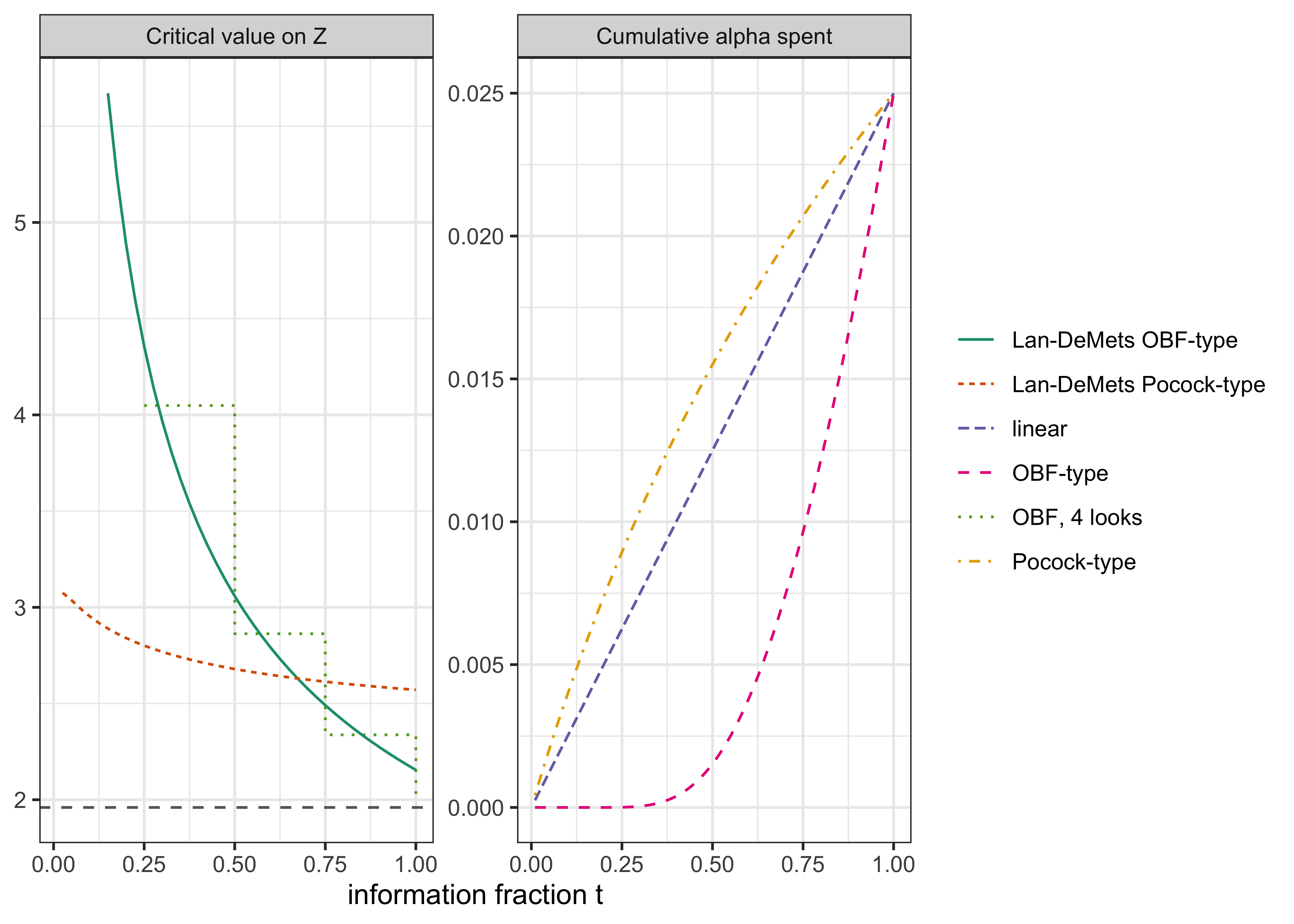
tt <- (1:40) /40; t4 <- (1:4) /4; tg <-seq(0.01, 1, length.out =100)pl <-c("Critical value on Z", "Cumulative alpha spent")spend_obf <-function(t) 2*pnorm(-qnorm(0.9875) /sqrt(t))spend_poc <-function(t) 0.025*log(1+ (exp(1) -1) * t)d <-rbind(data.frame(p = pl[1], t = tt, y =gs_spending_boundary(tt, spending ="ld_obf"), g ="Lan-DeMets OBF-type"),data.frame(p = pl[1], t = tt, y =gs_spending_boundary(tt, spending ="ld_pocock"), g ="Lan-DeMets Pocock-type"),data.frame(p = pl[1], t = t4, y =gs_boundary(4), g ="OBF, 4 looks"),data.frame(p = pl[2], t = tg, y =spend_obf(tg), g ="OBF-type"),data.frame(p = pl[2], t = tg, y =spend_poc(tg), g ="Pocock-type"),data.frame(p = pl[2], t = tg, y =0.025* tg, g ="linear"))d$y[d$p == pl[1] & d$y >6] <-NA# first looks: boundaries beyond the plotted rangeggplot(d, aes(t, y, colour = g, linetype = g)) +geom_step(data =subset(d, g =="OBF, 4 looks")) +geom_line(data =subset(d, g !="OBF, 4 looks")) +geom_hline(data =data.frame(p = pl[1], y =1.96), aes(yintercept = y), linetype ="dashed", colour ="grey40") +facet_wrap(~p, scales ="free_y") +scale_colour_brewer(palette ="Dark2") +labs(x ="information fraction t", y =NULL, colour =NULL, linetype =NULL) +theme_bw()
Figure 11.1: Left: critical values on the Z scale against the information fraction for four designs with one-sided alpha 0.025 and a fixed 1.96 for reference (the dashed line is the unadjusted cutoff that the repeated-testing table shows to be invalid). Right: cumulative alpha spent as a function of the information fraction by the two Lan-DeMets spending functions. Lan-DeMets boundaries were computed at 40 looks to approximate continuous monitoring.
Other boundary families
The Wang-Tsiatis family is not the only one. Armitage’s sequential plans (Peter Armitage 1954) were among the first proposed for medicine: two boundaries on a plot of the accumulated treatment difference against the accumulated information. The closed (restricted) plans, which end at a maximum sample size, are in Armitage’s later work (Peter Armitage 1960). Whitehead’s triangular test (Whitehead and Stratton 1983) is a closed alternative to Wald’s test of Section 11.8.4: the boundaries converge to a point at the maximum information, so the trial always ends with a decision, and the expected sample size under the design alternative is well below that of a fixed design. EOLIA (Section 11.12) is the book’s real trial that used it.
Pampallona and Tsiatis (Pampallona and Tsiatis 1994) added futility boundaries to the Wang-Tsiatis family, Emerson and Fleming (Emerson and Fleming 1989) gave symmetric designs between the O’Brien-Fleming and Pocock shapes, and Kittelson and Emerson (Kittelson and Emerson 1999) unified these in one family with efficacy and futility boundaries. Every member is evaluated by the recursion above and compared by the same properties: the maximum sample size, the expected sample size under the null and the alternative, and the stopping probabilities at each look. A design is chosen by weighing those properties against the protocol’s needs, not by ranking the families. Emerson, Kittelson and Gillen (Emerson, Kittelson, and Gillen 2007) set out this frequentist evaluation of group sequential designs (power, sample size and stopping probabilities across the family), and it is the same one the bayestrials package applies to the book’s Bayesian rules, so that a Bayesian design is compared with these on the same terms.
11.5 Spending functions and the information fraction
The designs above assume that the looks are at exact multiples of one quarter of the information. Real trials are not like that. Enrollment is irregular, events arrive when they arrive, and a DMC meeting is scheduled for the first Tuesday of a quarter and finds 47 percent of the planned events, not 50. A boundary computed for a \(t\) that did not occur is wrong.
Lan and DeMets (1983; see also Kim and DeMets 1987 for the power family \(\alpha^*(t) = \alpha t^{\rho}\)) resolved this by changing what is fixed in advance. Instead of fixing the boundaries, fix a spending function \(\alpha^*(t)\), a nondecreasing function with \(\alpha^*(0) = 0\) and \(\alpha^*(1) = \alpha\), which says how much of the total type I error may have been used up by the time the information fraction reaches \(t\). At the look with information fraction \(t_k\) the boundary \(b_k\) is the one for which the cumulative probability of crossing so far equals \(\alpha^*(t_k)\). Two spending functions mimic the classical designs (the right panel of Figure 11.1): \[
\alpha^*_{\text{OBF}}(t) = 2\{1 - \Phi(z_{\alpha/2}/\sqrt{t})\}, \qquad
\alpha^*_{\text{Pocock}}(t) = \alpha \log\{1 + (e - 1)\,t\}.
\tag{11.3}\] The first spends almost nothing until \(t\) is large (at \(t = 0.5\) it has spent about \(0.0015\) of the \(0.025\)), and the second spends steadily. The rule is that the function is in the protocol, not the number or times of the looks, and the boundary is computed at each look from the realized information fraction, using the previous boundaries as they were actually applied. Because the recursion needs only the past boundaries and the current \(t\), the calculation does not require knowing how many looks will occur. The only restriction is that the timing of looks must not depend on the observed treatment effect.
The calculation shows the point. Four looks planned at \(t = 0.4, 0.6, 0.8, 1\) (the design used in module 07 of the book’s companion online lab, https://nytel.ai/testing/07-interim-looks.html) have an O’Brien-Fleming-type boundary at the second look of \(2.68\). If enrollment falls behind and the second look takes place at \(t = 0.55\), the boundary at that look becomes \(2.82\), and the later boundaries move slightly. The total error is \(0.025\) and \(0.025\) in the two cases.
Two cautions belong with this flexibility. First, the information fraction at the final analysis is \(1\) only if the trial reaches its planned size; a trial that stops short, for example because event accrual is slower than planned, must decide in the protocol whether the remaining alpha is spent at the last look actually held. Second, the final analysis of a Lan-DeMets design is valid even if the interim looks turn out not to occur at the planned fractions, but the sample size was chosen for a particular plan, and the power calculation assumed a particular boundary.
TipAlpha is distributed, not consumed
Interim looks are widely believed to “cost alpha”. They do not in total: the trial still has one-sided \(0.025\) for the whole experiment, and the spending function says where in the trial it lives. A final critical value of \(2.02\) instead of \(1.96\) records where the rest of the alpha went. What requires adjustment is the action taken on the interim data. A stop for superiority spends alpha. A stop for futility does not, and, if binding, it gives some back. A DMC that reviews safety without an efficacy comparison does not touch alpha at all.
11.6 Futility boundaries: binding and non-binding
An efficacy boundary is the upper edge of the continuation region. A futility boundary is the lower edge: if the interim statistic is below it, the trial is stopped because the treatment is unlikely to show benefit. Futility stops reduce the chance of a false positive (a trial stopped for futility cannot later cross the upper boundary), and they shorten trials of useless drugs. They differ in what the protocol says about whether the DMC must obey them.
A binding futility boundary is part of the design. If it is crossed the trial stops, and the type I error is computed on the assumption that the trial does. The reduction in type I error can then be used to lower the efficacy boundaries a little.
A non-binding futility boundary is a guideline. The DMC may recommend stopping, or may decline to, and the type I error is computed as though the futility boundary did not exist. Because ignoring it can only increase the chance of crossing the efficacy boundary, the type I error is at most \(\alpha\) whether the committee follows the guideline or not.
The conservative position of the traditional world, and what the regulatory documents generally encourage, is the non-binding rule, because a DMC’s decision to continue a trial should never be what invalidates its type I error. The cost shows up in the power calculation, which should be done as if the futility rule were followed (otherwise the stated power is not what the trial would achieve if it were). The cell below uses a simple rule on a four-look O’Brien-Fleming design: stop for futility at looks 1, 2, 3 if the standardized statistic is below zero.
Show the R code
t <- (1:4) /4; fut <-c(0, 0, 0, -Inf)b_nb <-gs_boundary(4, type ="obf")cb <-uniroot(function(cc) gs_power(t, cc /sqrt(t), fut) -0.025, c(1.5, 4), tol =1e-10)$rootxi <-gs_power_drift(t, b_nb, target =0.90)des <-list("no futility rule"=list(b_nb, NULL), "non-binding"=list(b_nb, fut), "binding"=list(cb /sqrt(t), fut))tab <-do.call(rbind, lapply(names(des), function(nm) { b <- des[[nm]][[1]]; lo <- des[[nm]][[2]]data.frame(design = nm, type1_if_obeyed =round(gs_power(t, b, lo), 4), type1_if_ignored =round(gs_power(t, b), 4),efficacy_bounds =paste(round(b, 2), collapse =", "), power =round(gs_power(t, b, lo, xi), 3),E_H1 =round(gs_expected_information(t, b, lo, xi), 3), E_H0 =round(gs_expected_information(t, b, lo, 0), 3))}))knitr::kable(tab)
Table 11.3: Effect of a futility boundary (stop if Z < 0 at looks 1 to 3) on an O’Brien-Fleming design with four equally spaced looks. ‘Binding’ lowers the efficacy boundaries to restore alpha = 0.025 assuming the rule is obeyed; ‘non-binding’ keeps the efficacy boundaries.
design
type1_if_obeyed
type1_if_ignored
efficacy_bounds
power
E_H1
E_H0
no futility rule
0.0250
0.0250
4.05, 2.86, 2.34, 2.02
0.900
0.751
0.997
non-binding
0.0229
0.0250
4.05, 2.86, 2.34, 2.02
0.869
0.713
0.544
binding
0.0250
0.0274
3.98, 2.81, 2.3, 1.99
0.874
0.705
0.543
Under the null, the futility rule stops the trial early about 69 percent of the time (50 percent at the first look alone), and the expected information used falls from 100 percent of the planned total to about 54 percent. Under the alternative the rule costs 3 percentage points of power in this example, the difference between 0.90 and 0.87, because some trials with a true benefit have a negative interim statistic by chance. A binding rule recovers about 0.5 of a percentage point of that loss by lowering the efficacy boundaries (to \(3.98, 2.81, 2.30, 1.99\)). It does so at the price that, if the committee overrides it, the type I error is no longer controlled, which is why many sponsors and most regulators prefer non-binding rules for confirmatory trials. A threshold of “\(Z < 0\)” is crude. In practice the futility criterion is usually a conditional power or a predictive probability, which is the subject of Chapter 15. Conditional power, introduced for trials as stochastic curtailment by Lan, Simon and Halperin (Lan, Simon, and Halperin 1982), is defined and compared with the predictive probability in Section 15.1. Two real trials that stopped for futility, EOLIA (under a triangular sequential design) and the critically ill cohort of the heparin multiplatform trial (under a Bayesian rule), are described in Section 11.12.
11.7 What a DMC does
A DMC (the older terms are DSMB, data safety monitoring board, and IDMC) is a small independent group, typically three to seven members, consisting of clinicians in the therapeutic area and at least one statistician, which reviews accumulating data during the trial and recommends to the sponsor whether to continue, modify, or stop. Ellenberg, Fleming and DeMets (2019) is the standard book, and FDA’s 2006 guidance (U.S. Food and Drug Administration 2006), and its February 2024 draft revision, not final (U.S. Food and Drug Administration 2024). The practice that matters for the statistical design is as follows.
Separation of roles. The DMC sees unblinded comparative data. The sponsor and the investigators do not. An independent statistical group (not the trial’s analysis team) prepares the closed reports for the DMC, and its work is walled off from the rest of the sponsor. The FDA guidance and the adaptive designs guidance both stress that access to interim comparative results by people who can influence the trial’s conduct compromises its integrity, and in a confirmatory trial a compromise of that kind can make the result uninterpretable. The 2019 guidance names trial integrity as the fourth principle for adaptive designs.
The charter. Before the first patient is enrolled, the DMC charter fixes the committee’s membership, meeting schedule, the content of the open and closed reports, the stopping guidelines, and the communication path to the sponsor. The stopping guidelines are the boundaries of this chapter: efficacy (for example, an O’Brien-Fleming-type Lan-DeMets spending function at the planned information fractions), futility, and safety. For safety the boundaries are usually not formal tests of an alpha-controlled hypothesis, and are typically reviewed with different weight.
Boundaries are guidelines. A DMC is not an automaton (the stop for harm of the Women’s Health Initiative estrogen plus progestin trial, in Section 11.12, was a committee recommendation). A boundary crossed by a small margin at an early look, with consistency across secondary endpoints and no safety signal, will often be treated differently from the same crossing with an inconsistent picture. The reverse also holds: a DMC may recommend stopping for harm without a boundary having been crossed. Discretion does not by itself inflate the efficacy error. Declining to stop after an efficacy crossing, or stopping for safety, leaves the type I error at most \(\alpha\) as long as a claim of success remains restricted to crossings of the prespecified boundary. What can damage the guarantee is a decision that uses comparative data outside the rule, and conduct that compromises integrity. The type I error is a statement about the rule as written, and the discretion the DMC retains is a reason that the boundaries are stringent early and permissive late. A stringent early boundary means that a DMC’s judgment will be exercised in few cases, at times when the evidence is overwhelming.
Why early stops overestimate. A trial that stops at an early look because it crossed a boundary stopped because the observed effect was large, and a large observed effect is more likely to be a positive deviation from the truth. The point estimate at an early stop is biased away from the null, an effect documented by Pocock and Hughes (1989). The bias is bigger the smaller the trial and the earlier the stop. Adjusted estimators exist, but the practical message is to read an early-stopped estimate with the sample size and the confidence interval in view, and to say so in the report. Module 07 of the companion lab makes the same point in its takeaways. The empirical size of the effect is documented in Section 11.12: in a meta-epidemiological study of 91 trials stopped early for benefit, the ratio of relative risks against matched trials that were not stopped was \(0.71\)(Bassler et al. 2010).
Confidentiality and what the sponsor learns. The sponsor learns only the recommendation. A recommendation to continue unchanged discloses little. A recommendation to stop discloses much, and a recommendation to modify, for example to drop an arm or enrich a population, can disclose a great deal. This is why a design in which the sponsor can see the interim effect (for example, to resize the sample) needs the extra controls that Chapter 23 discusses.
Stopping boundaries in the 2019 guidance. The group sequential design with a prespecified spending function is the simplest case of an adaptive design in the sense of the 2019 guidance, and one for which the type I error is controlled by a known calculation without simulation. For this reason regulators treat it as well understood, and it is the standard against which a Bayesian monitoring plan will be compared: sponsors who propose a Bayesian monitoring rule are asked to show its type I error under the null and its power, by simulation, and the group sequential design is the benchmark that sets the expectation of “what good looks like”.
TipIn the protocol: interim analysis section (traditional)
Interim analyses. One interim analysis for efficacy and futility will be performed when 50% of the planned primary events have been observed, and a second at 75%. Efficacy will be assessed using a Lan-DeMets spending function of the O’Brien-Fleming type at overall one-sided \(\alpha = 0.025\), with boundaries recomputed from the observed number of events at each analysis. A non-binding futility guideline of conditional power below 10% under the design alternative applies at the first analysis. The Independent Data Monitoring Committee will review unblinded data prepared by an independent statistician and will recommend continuation, modification or termination; it is not bound by these guidelines. The sponsor will not have access to comparative data before database lock.
11.8 The Bayesian sequential problem
We now pose the monitoring problem the Bayesian way. The question is not “how do we divide up \(\alpha\)”, but “what should be done at each look, given what we have seen and what stopping costs”. Three observations frame the answer: the posterior is unaffected by the stopping rule, the error rate is not, and the stopping rule itself is a decision problem with a solution.
The posterior does not depend on the stopping rule
Let the trial stop at a random time \(T\) determined by a rule that depends only on the data so far. The likelihood of the observed data under a parameter \(\theta\) is, for the observations that were made, the product of the densities of those observations times the probability that the stopping rule would have continued until \(T\) and stopped there. The second factor depends only on the data, not on \(\theta\), so it cancels in the posterior. The posterior after stopping at \(T\) with data \(y_{1:T}\) is exactly the posterior one would have computed had the sample size been fixed at \(T\) in advance. This is the likelihood principle in its sequential form, the stopping rule principle (Edwards, Lindman, and Savage 1963; Cornfield 1966; Berry 1987; Berger and Wolpert 1988), and it is the foundation of the Bayesian claim that “you may look as often as you like”. The heparin multiplatform trial of Section 11.12 monitored on exactly this kind of posterior rule.
The same is not true of a frequentist \(p\)-value or a confidence interval, because these are tail probabilities over the other data sets that might have been seen, and which other data sets are possible depends on the stopping rule. That is why the rest of this chapter has needed a boundary table, and why a Bayesian analyst and a frequentist analyst looking at the same interim data will report different things. Armitage (P. Armitage, McPherson, and Rowe 1969) was the long-standing voice of the other side, holding that the logic of repeated significance tests applies to the trial and that a conclusion must account for how often the data were examined.
A small example makes the difference concrete. A trial ends with 15 responders among 20 patients, and the null response probability is one half. If 20 was the planned sample size, the one-sided \(p\)-value is 0.021. If instead the plan was to keep enrolling until the fifth non-responder, the same sequence of 20 patients ends the trial at the same place, but the \(p\)-value is now 0.01, because the sample space of other trials that might have been run is different. The likelihood is the same up to a constant, so under a flat prior the posterior is Beta(16, 6) in both cases and \(\Pr(\theta > 0.5 \mid \text{data}) = 0.987\) (for the response probability \(\theta\)). That one result is the heart of the dispute in the sources cited above: the frequentist says the stopping plan is part of the evidence, the Bayesian says it is not, and the clinician needs only to know which of the two the protocol and the regulator are using. For the calibrated designs used here, simulate type I error and power under the planned stopping rule. Other Bayesian success criteria are discussed in Chapter 3.
The simulation below shows both facts (Table 11.4). The true effect \(\theta\) is drawn from a prior \(N(0, 0.5^2)\), data are \(N(\theta, 1)\) per patient, and the committee monitors after every patient to \(n = 400\), stopping at the first time the posterior probability that \(\theta > 0\) reaches \(0.975\).
Show the R code
set.seed(2024)N <-400; tau0 <-0.5; cc <-0.975; prec <- (1:N) +1/ tau0^2run <-function(theta) { # Pr(theta > 0 | S_n) under the prior N(0, tau0^2) S <-matrix(rnorm(length(theta) * N, theta), ncol = N)for (j in2:N) S[, j] <- S[, j -1] + S[, j] pp <-pnorm(sweep(S, 2, sqrt(prec), "/")); hit <- pp >= cc st <-rowSums(hit) >0; first <-max.col(hit, "first")list(stopped = st, pp = pp[cbind(seq_along(theta), first)])}theta <-rnorm(20000, 0, tau0); a <-run(theta); a0 <-run(rep(0, 20000))lk <-c(mean(a$stopped), mean(a$pp[a$stopped]), mean(theta[a$stopped] >0), mean(a0$stopped))knitr::kable(data.frame(Quantity =c("P(stop for benefit), prior-averaged", "Mean claimed posterior probability at stop","Fraction with theta > 0 among stopped", "P(declare benefit), point null theta = 0"), Value = lk), digits =3, align ="lr")
Table 11.4: A Bayesian monitoring rule (stop at the first patient at which Pr(theta > 0 | data) >= 0.975, at most 400 patients). Calibration under the prior: among trials that stop for benefit, the mean claimed posterior probability matches the fraction in which theta really is positive. Frequentist error under a point null: the same rule declares benefit far more often than 2.5%.
Quantity
Value
P(stop for benefit), prior-averaged
0.453
Mean claimed posterior probability at stop
0.981
Fraction with theta > 0 among stopped
0.979
P(declare benefit), point null theta = 0
0.175
Among the trials that stop, the claim made at the stopping time (the mean posterior probability, about \(0.98\)) matches the fraction of those trials in which the effect is truly positive. Bayesian calibration under the prior survives optional stopping untouched. But if the null is exactly true, the same rule declares benefit in about \(17.5\%\) of trials: an error rate seven times the usual \(2.5\%\) for a rule whose posterior probabilities are all correct. Both statements are right and they answer different questions. The first is a statement averaged over the prior, the second is conditional on one value of \(\theta\), which is the way a type I error is defined, and the requirement of the error-calibrated approach used in this book (Chapter 3) is on the second. This is the central tension of the Bayesian approach to monitoring. Its frequentist error rate must be computed by simulation under the design, which is the work of Chapter 14, and, if the rule is to be a basis for approval, the threshold \(c\) is tuned until that error is acceptable. Note that the point null in the table is an extreme case: under a continuous prior, an exactly-zero effect has no prior mass, and the first three rows are what the sponsor is protected by when the prior is a fair description of the program.
A short history of Bayesian monitoring
The Bayesian monitoring rule of this chapter has a lineage. Freedman, Lowe and Macaskill (L. S. Freedman, Lowe, and Macaskill 1984) proposed stopping rules that incorporate clinical opinion as a prior, and Freedman and Spiegelhalter (Laurence S. Freedman and Spiegelhalter 1989) compared Bayesian monitoring with group sequential methods. Spiegelhalter, Freedman and Parmar (Spiegelhalter, Freedman, and Parmar 1994) proposed the skeptical and enthusiastic reference priors of Section 8.3 and a range of equivalence, and a monitoring rule that stops when the posterior probability of benefit, or of exceeding that range, passes a threshold. Grossman and colleagues (Grossman et al. 1994) gave a unified method for monitoring and analyzing controlled trials, and Fayers, Ashby and Parmar (Fayers, Ashby, and Parmar 1997) wrote the tutorial. Berry (Berry 1985, 1987) argued from the likelihood principle that interim analyses should not be penalized, and Rosner and Berry (Rosner and Berry 1995) gave a Bayesian group sequential design for a multiple-arm trial. The rule of this chapter keeps their posterior and adds the calibration of its operating characteristics by simulation (Chapter 14) that a regulator asks for. The wider history of Bayesian trial design is in Section 1.9.
The Bayes sequential decision problem
Writing the stopping rule as part of the decision gives the Bayes sequential problem. A design is a pair \((T, d)\): a stopping time \(T \le N_{\max}\) adapted to the data and a terminal decision \(d\) made at \(T\). Let \(\ell(\theta, d)\) be the loss from the terminal decision (the cost of approving an ineffective drug, or of abandoning an effective one) and let each enrolled patient carry a cost \(\kappa(\theta)\), so the total loss is \(\ell(\theta, d) + \kappa(\theta)\,T\). The Bayes rule minimizes the expected total loss under the prior.
The solution is dynamic programming on the posterior. Because the posterior depends on the data only through a sufficient statistic (the count of successes for binary data, the score \(S_n\) for a normal mean), the state at look \(n\) is the pair \((n, S_n)\). Let \(V(n, S)\) be the minimal expected future loss in that state. At the horizon only the terminal decision remains. Before the horizon the committee compares stopping now with taking one more observation and acting optimally thereafter, \[
V(n,S) = \min\Bigl\{\min_d \mathbb{E}[\ell(\theta,d) \mid n, S],\;\; \mathbb{E}[\kappa(\theta) \mid n, S] + \mathbb{E}_{\text{pred}}\bigl[V(n+1, S+X_{n+1})\bigr]\Bigr\},
\tag{11.4}\] with \(V(N_{\max}, S) = \min_d \mathbb{E}[\ell(\theta,d) \mid N_{\max}, S]\). This is the construction given by Sokolova, Sokolov and Polson (2026). A decision tree over \(N_{\max}\) steps has exponentially many branches, but indexed by the sufficient statistic it becomes a table over states, filled by backward induction. For a single-arm binary endpoint the states \((n, S)\) form a lattice with order \(N_{\max}^2\) entries. For a two-arm binary trial the state is a pair of success counts at each \(n\), and the lattice is cubic in \(N_{\max}\) (Chapter 15). For normal data the statistic is continuous and the recursion is evaluated on a numerical grid. The set of states \((n, S)\) in which stopping is optimal is the stopping region, and its boundary is the Bayes boundary. Two properties follow in the examples of this book. The continuation region narrows toward the horizon, because the option value of another observation shrinks as the number of remaining observations does; its exact shape depends on the loss and the sampling cost, and it need not be triangular. And early in the trial the boundary is wide, since a decision that is premature is expensive and the patient cost is small relative to what another look can buy.
The reduction to a sufficient statistic is what makes this computable in a trial setting, and it is the subject of Chapter 15, where the loss is replaced by the sponsor’s operational criterion (predictive probability of success) and the backward induction is implemented. For this chapter the point is the contrast. The traditional design chooses the boundary to control a type I error and then asks what it costs. The Bayes design chooses the boundary to minimize an expected loss and then asks what error rates it has. For the error-calibrated approach used in this book, the second must be turned into the first, by simulation, before it can be a primary analysis. The FDA’s draft Bayesian guidance of January 2026 describes calibration to a type I error rate as one of its routes, beside direct interpretation of posterior probabilities and decision-theoretic criteria (see Chapter 14).
Wald’s test and the large deviation ledger
The oldest sequential procedure, and the reference point for everything above, is Wald’s sequential probability ratio test (SPRT) (Wald 1945), which Barnard (Barnard 1946) developed independently. For the simple hypotheses \(H_0\) and \(H_1\) with densities \(p_0\) and \(p_1\), accumulate the log likelihood ratio \(\Lambda_n = \sum_{i\le n} \log\{p_1(X_i)/p_0(X_i)\}\) and stop at the first time it leaves the interval \((\log B, \log A)\) with \(A = (1-\beta)/\alpha\) and \(B = \beta/(1-\alpha)\), accepting \(H_1\) at the upper edge and \(H_0\) at the lower. This is exactly the posterior odds rule of a Bayesian with a two-point prior, and Wald and Wolfowitz (1948) proved that among all tests with the same error probabilities it has the smallest expected sample size under both hypotheses.
For the normal mean with unit variance, \(H_0: \theta = 0\) against \(H_1: \theta = 0.2\), with \(\alpha = 0.025\) and \(\beta = 0.10\), a fixed-sample test needs \((z_\alpha + z_\beta)^2/\theta^2 = 263\) patients. Wald’s approximation to the expected sample size under \(H_1\) is \[
\mathbb{E}_1[T] \approx \frac{(1-\beta)\log\{(1-\beta)/\alpha\} + \beta \log\{\beta/(1-\alpha)\}}{\mathrm{KL}(P_1 \| P_0)},
\tag{11.5}\] where \(\mathrm{KL} = \theta^2/2 = 0.02\) per patient is the Kullback-Leibler divergence. The cell below evaluates it and checks it by simulation.
Show the R code
th <-0.2; al <-0.025; be <-0.10A <-log((1- be) / al); B <-log(be / (1- al)); KL <- th^2/2set.seed(1945)sprt <-function(mu, reps =20000) { n <-integer(reps); acc <-logical(reps)for (i inseq_len(reps)) { L <-0; k <-0Lwhile (L > B && L < A) { L <- L + th *rnorm(1, mu) - th^2/2; k <- k +1L } n[i] <- k; acc[i] <- L >= A }list(n = n, acc = acc)}s1 <-sprt(th); s0 <-sprt(0)fixed <- (qnorm(1- al) +qnorm(1- be))^2/ th^2knitr::kable(data.frame(fixed_n =round(fixed),wald_approx =round(c(((1- be) * A + be * B) / KL, -((1- al) * B + al * A) / KL)),simulated_mean =round(c(mean(s1$n), mean(s0$n))),p95 =c(quantile(s1$n, 0.95), quantile(s0$n, 0.95)),rejects_H0 =round(c(mean(s1$acc), mean(s0$acc)), 3), row.names =c("under H1", "under H0")))
Table 11.5: Wald’s SPRT for a normal mean, theta=0.2 against 0, alpha=0.025, beta=0.10. Wald’s approximation against 20,000 simulated trials; the fixed-sample size for the same error rates is 263. Simulation overshoots the boundary, which is why its error rates are slightly better than nominal and its sample sizes slightly higher than the approximation.
fixed_n
wald_approx
simulated_mean
p95
rejects_H0
under H1
263
150
159
360
0.913
under H0
263
107
113
297
0.023
In the simulation the SPRT stops on average at about 159 patients when the drug works (a 40 percent saving against 263; Wald’s approximation says 150) and at about 113 when it does not (approximation 107). Three features of Equation 11.5 define what we call the large deviation ledger. The numerator, \(\log\{(1-\beta)/\alpha\}\) and its companion, is a fixed quantity of evidence, measured in nats and set by the error levels alone, not by the size of the trial. The denominator is a Kullback-Leibler divergence, the rate at which evidence accrues, linearly in \(n\) and at a speed fixed by the alternative. And the governing relation \(n\,\mathrm{KL} \asymp \log(1/\alpha)\) is the Chernoff-Stein relation of large deviation theory. All of it is a statement at exponential speed: to rule out a null with probability error \(\alpha\) requires evidence \(\log(1/\alpha)\), and evidence comes at rate \(\mathrm{KL}\).
Two cautions apply to the SPRT in a trial. Its sample size has no upper bound: the 95th percentile under \(H_1\) is above the fixed-sample size, and a few trials run for several times the fixed size. A trial must have a maximum, which is why group sequential designs, with a hard end, are the standard. And it tests two simple hypotheses, whereas a trial’s alternative is composite. The remedy is to place a prior on the effect and use the mixture likelihood ratio, which brings us back to the Bayes factor and to the three tolls.
11.9 The three deviation scales
Set up
Let \(I_n\) be the Fisher information about \(\theta\) after \(n\) observations, \(\hat\theta_n\) the efficient estimator, \(Z_n = \hat\theta_n \sqrt{I_n}\) the standardized score, and \(S_n = \hat\theta_n I_n\) the accumulated score, which behaves like Brownian motion with drift \(\theta\) in information time. For a time-to-event endpoint with \(d\) events and \(\theta = -\log \mathrm{HR}\), the usual approximation is \(I_n = d/4\). Put a prior \(\theta \sim N(0, \tau^2)\) on the alternative. The mixture Bayes factor for the alternative against the point null is \[
\mathrm{BF}_n = (1 + I_n\tau^2)^{-1/2} \exp\Bigl\{\frac{Z_n^2}{2}\cdot\frac{I_n\tau^2}{1+I_n\tau^2}\Bigr\}, \qquad
2\log \mathrm{BF}_n = Z_n^2 - L_n - \frac{Z_n^2}{1+q}, \qquad q = I_n\tau^2,
\tag{11.6}\] where \[
L_n = \log(1 + I_n\tau^2) \sim \log I_n
\tag{11.7}\] is the Ockham penalty of Chapter 7, the price for integrating the parameter out. The remainder \(Z_n^2/(1+q)\) is exact, not \(o(1)\) in general (under a fixed nonzero effect it converges to \(-\theta^2/\tau^2\) in \(2\log\mathrm{BF}_n - Z_n^2 + L_n\)); it is negligible near the boundaries below, where \(Z_n^2 = O(\log q)\). This is the finite-sample form of the Schwarz penalty (Schwarz 1978). Under the null \(\mathbb{E}_0[\mathrm{BF}_n] = 1\) and run over time \(\mathrm{BF}_n\) is a nonnegative martingale (a test martingale, which is the subject of Chapter 12), so that Ville’s inequality (Ville 1939) gives \(\Pr_0(\sup_n \mathrm{BF}_n \ge 1/\alpha) \le \alpha\). The same statistic is therefore the Bayes factor of a Bayesian and the e-process of an anytime-valid analyst. They differ in where they put the bar.
The three tolls
NoteResult: evidence tolls (Polson and Sokolov)
With \(L_n\) as in Equation 11.7 and \(q = I_n\tau^2\), the three calibrations act, for a one-sided claim (so \(Z_n > 0\)), when \[
\begin{aligned}
&\text{fixed level } \alpha: && Z_n \ge z_\alpha,\\
&\text{Bayes, threshold } b: && Z_n^2 \ge \Bigl(1 + \tfrac{1}{q}\Bigr)\{\log(1+q) + 2\log b\} \approx L_n + 2\log b,\\
&\text{anytime valid } \alpha: && Z_n^2 \ge \Bigl(1 + \tfrac{1}{q}\Bigr)\{\log(1+q) + 2\log(1/\alpha)\} \approx L_n + 2\log(1/\alpha).
\end{aligned}
\tag{11.8}\] The middle and last forms are exact for the symmetric normal mixture, and the approximations on the right are large-information forms (\(q \to \infty\)). For this normal-mixture construction the anytime-valid rule requires \(2\log(1/\alpha)(1 + 1/q)\) more, in squared standardized units, than the Bayes rule at \(b = 1\), which is approximately the constant \(2\log(1/\alpha) = 7.38\) at large information. These are properties of this construction and not universal costs of anytime validity.
NoteTechnical note: proof of the tolls
The first is the definition of the one-sided fixed-level test. For the second, the rule acts when \(\mathrm{BF}_n \ge b\), and Equation 11.6 gives \(2\log \mathrm{BF}_n = \{q/(1+q)\}Z_n^2 - \log(1+q)\), so the event is \(Z_n^2 \ge (1+1/q)\{\log(1+q) + 2\log b\}\), which is \(Z_n^2 \ge L_n + 2\log b + o(1)\) as \(q \to \infty\) (the factor \(1 + 1/q\) multiplies a quantity that grows only logarithmically). Setting \(b = 1/\alpha\) gives the third. The ratio of the two squared bars is \(\{L_n + 2\log(1/\alpha)\}/L_n = 1 + 2\log(1/\alpha)/\log(1 + I_n\tau^2)\), which tends to one, but only as \(1/\log n\): the additive excess never shrinks.
In words. A single fixed-level test asks for a score of \(1.96\) however much information there is, so that its squared bar is the constant \(z_\alpha^2 = 3.84\). A Bayesian who wants posterior odds of \(b\) for the alternative needs a squared score that grows like \(\log n\), because a bigger sample makes a precisely-zero null a sharper target against a diffuse alternative. And, in this normal-mixture construction, a rule that must stay valid however and whenever it is stopped pays approximately \(2\log(1/\alpha)\) on top of the Bayesian bar at large information, with \(2\log 40 = 7.38\) at \(\alpha = 0.025\) (exactly \(7.38(1 + 1/q)\)).
Table 11.6: The Ockham penalty L_n = log(1 + I tau^2) and the bars on Z at prior scale tau = 0.25, with alpha = 0.025. The exact bars of the symmetric normal mixture carry the factor (1 + 1/q), q = I tau^2; the columns labeled approx. are the large-information forms sqrt(L_n + 2 log b) and sqrt(L_n + 7.378), shown for comparison. The unadjusted bar is 1.96 throughout. Ratio is the ratio of the squared anytime-valid and Bayes bars.
Information
Ockham L
Fixed
Bayes (exact)
Anytime (exact)
Bayes (approx.)
Anytime (approx.)
Ratio
25
0.94
1.96
1.24
3.69
0.97
2.88
8.84
50
1.42
1.96
1.37
3.41
1.19
2.97
6.21
100
1.98
1.96
1.52
3.29
1.41
3.06
4.72
200
2.60
1.96
1.68
3.28
1.61
3.16
3.83
400
3.26
1.96
1.84
3.33
1.81
3.26
3.26
1000
4.15
1.96
2.05
3.42
2.04
3.40
2.78
4000
5.53
1.96
2.36
3.60
2.35
3.59
2.34
Two things stand out. The Bayes bar with \(b = 1\) is below the unadjusted bar at small information, because the Ockham penalty \(L_n\) is small while the information is small relative to the prior precision \(1/\tau^2\), but it overtakes \(1.96\) once \(L_n\) exceeds \(z_\alpha^2 = 3.84\), that is asymptotically for \(I_n \tau^2 > 46\) (for a unit-information prior, \(I_n\tau^2 = n\) and the condition is \(n > 46\), while at \(\tau = 0.25\) it needs \(I_n > 730\), about 2,900 events); the exact bar of the stated mixture crosses \(1.96\) at \(q \approx 41.6\). From there on it keeps rising. Realistic confirmatory trials need not be past this point. Past that point the uncalibrated Bayes-factor bar is above the unadjusted bar, and the Bayesian saving is not a saving against a single unadjusted look. What matters in practice is the comparison of calibrated rules, which Chapter 21 and Chapter 12 make for the SELECT reconstruction: a single unadjusted look would cross at 309 events on the mean path, while among simulated trials that declare efficacy the calibrated Bayesian rule stops at a median of 464 events (power 0.95, realized type I error 2.5%). This is the book’s thesis on its sharpest edge: the saving comes from monitoring and from using prior information, not from a lower bar. Second, the exact anytime-valid bar for this construction is higher again, at 3.3 to 3.7 across the range, by a surcharge of \(7.38(1 + 1/q)\) that is approximately constant in \(n\) and that dominates \(L_n\) over the whole range of information that trials reach.
Where the surcharge comes from
For this normal-mixture construction the approximate boundary surcharge is not a convention: it comes from fixing the bar at \(\log(1/\alpha)\) in log-evidence, and the mechanism is the exponential bound of the preceding section. It is a cost of this construction and of this comparison, not a lower bound for all anytime-valid procedures. Realizable boundaries with iterated-logarithm rates exist (Robbins 1970) and behave differently.
NoteTechnical note: the surcharge is the Chernoff toll
Let \(M_n\) be a nonnegative martingale with \(M_0 = 1\). Ville’s inequality \(\Pr(\sup_n M_n \ge 1/\alpha) \le \alpha\) is Markov’s inequality applied to \(M_n\) at a stopping time. For the exponential martingale \(M_n = \exp(\lambda S_n - n\lambda^2/2)\) the first passage of \(M_n\) to \(1/\alpha\) is the first time the cumulative log likelihood ratio reaches \(\log(1/\alpha)\). Under an alternative with per-observation Kullback-Leibler divergence \(\mathrm{KL}\), Wald’s identity gives \(\mathbb{E}[T_\alpha] = \{\log(1/\alpha)/\mathrm{KL}\}(1 + o(1))\). The bar \(\log(1/\alpha)\) is fixed and evidence accrues linearly at rate \(\mathrm{KL}\), so the governing relation is \(n\,\mathrm{KL} \asymp \log(1/\alpha)\): the Chernoff-Stein relation, the large deviation ledger of the previous section.
The Bayes bar, by contrast, is not fixed. It is \(L_n \sim \log I_n\), and the governing relation is \[
n\theta^2 \asymp \log n,
\tag{11.9}\] the moderate deviation relation. Under it the type I error induced by a Bayes rule at threshold one tends to zero polynomially at a single analysis at \(n\), as \((n \log n)^{-1/2}\), rather than being pinned at a constant, a result of Polson and Sokolov (2026b). The three scales line up as follows.
Table 11.7: The three deviation scales.
scale
bar on \(Z_n^2\)
information required to decide
central limit, standard design
constant \(z_\alpha^2\)
\(n\theta^2 \asymp (z_\alpha + z_\beta)^2\)
moderate deviation, Bayes
\(\log n + C\), grows slowly
\(n\theta^2 \asymp \log n + C\)
large deviation, anytime valid
\(\log n + C + 2\log(1/\alpha)\)
\(n\theta^2 \asymp \log n + C + 2\log(1/\alpha)\)
The sample size formula of Chapter 9 is the first row; the second row is the sample size equation of that chapter (Equation 9.10) with the power margin \(z_\beta\) removed, as in Equation 11.12 below, and the third is the price of being valid at every stopping time.
The seventy percent result
NoteResult: required information
With per-observation standardized effect \(\theta\), the information needed to act satisfies \(n_{\mathrm{MD}}\theta^2 = \log n_{\mathrm{MD}} + C\) for the Bayes rule and \(n_{\mathrm{LD}}\theta^2 = \log n_{\mathrm{LD}} + C + 2\log(1/\alpha)\) for the anytime-valid rule, so the excess is the constant \[
n_{\mathrm{LD}} - n_{\mathrm{MD}} \approx \frac{2\log(1/\alpha)}{\theta^2},
\tag{11.10}\] and relative to the fixed-sample requirement \(n_{\mathrm{fix}} = (z_\alpha + z_\beta)^2/\theta^2\), \[
\frac{n_{\mathrm{LD}} - n_{\mathrm{MD}}}{n_{\mathrm{fix}}} \approx \frac{2\log(1/\alpha)}{(z_\alpha + z_\beta)^2} = \frac{7.38}{10.51} \approx 0.70
\tag{11.11}\] at \(\alpha = 0.025\) and 90 percent power, a large-information approximation of the boundary terms. The baseline is the uncalibrated Bayes-factor bar (posterior odds of one). The figure compares boundary terms asymptotically for this normal-mixture construction and is not an exact sample-size identity: subtracting the two sample-size equations adds a positive \(\log(n_{\mathrm{LD}}/n_{\mathrm{MD}})\) term. A calibrated Bayesian rule has already paid part of the surcharge, so calibration narrows the realized gap (see below).
Show the R code
al <-0.025; pw <-0.90num <-2*log(1/ al); den <- (qnorm(1- al) +qnorm(pw))^2
For this normal-mixture construction the approximate surcharge amounts to 70 percent of an entire conventional trial, measured against the uncalibrated Bayes-factor bar (posterior odds of one). That is the asymptotic ledger result, and calibration narrows it: a Bayesian rule whose threshold has been raised until its type I error is 2.5 percent pays part of the surcharge itself. In the SELECT reconstruction of Chapter 12 (true hazard ratio 0.80, at most 1,270 events), among simulated trials that declare efficacy, the calibrated Bayesian rule stops at a median of 464 events (power 0.95) and the e-value rule at 612 (power 0.83, realized type I error 0.6%), which is 32 percent more events and not seventy percent of a trial; SELECT’s planned two-look design stops at 817. Over all trials, counting those that never cross, the medians are 486 and 714. The result is stated per unit \(1/\theta^2\) and so does not depend on the effect size: it says the surcharge is a fixed multiple of the conventional sample size. It sits beside two consequences. First, because the ratio in the technical note tends to one, it is sometimes read as saying the anytime-valid penalty is asymptotically negligible. It is not, in practice, because the convergence is in \(1/\log n\) and the additive excess never shrinks. Second, none of this makes continuous monitoring a bad idea. It says what unrestricted monitoring costs for this construction, in the same currency as the group sequential designs of the first half: a design with four planned looks has a final bar of \(2.02\) and pays an inflation of \(2\) percent, and a design valid at every stopping time pays a surcharge that is a large fraction of a trial. A sponsor chooses how much flexibility to buy, and Chapter 12 takes up when it is worth buying all of it.
Four boundaries compared
The tolls say what each calibration asks for at a given information level. The same comparison can be made as a function of \(n\) on the \(Z\) scale, and it contains one surprise.
Table 11.8: Four boundaries on the standardized score. Fixed level z_alpha; moderate deviation sqrt(log n); iterated-logarithm shape sqrt(2 log log n); and the Robbins normal-mixture boundary, a realizable anytime-valid boundary at alpha = 0.025 with unit mixing scale, in the form used by Polson and Sokolov.
n
fixed
sqrt_log_n
sqrt_2loglog_n
robbins
5e+01
1.96
1.98
1.65
3.40
1e+02
1.96
2.15
1.75
3.48
5e+02
1.96
2.49
1.91
3.69
1e+03
1.96
2.63
1.97
3.78
1e+04
1.96
3.03
2.11
4.07
1e+05
1.96
3.39
2.21
4.35
1e+06
1.96
3.72
2.29
4.60
The ordering is not the obvious one. The iterated-logarithm rate, which is the shape any boundary valid at all times must have, grows more slowly than the moderate-deviation Bayes boundary: the ratio is \(1.34\) at a thousand observations and \(1.44\) at ten thousand. So the cheapest conceivable anytime-valid boundary, in shape, grows more slowly than the Bayes risk-optimal boundary for a fixed sample. Yet the realizable anytime-valid boundary, the Robbins mixture, sits well above both, at \(3.78\) where the Bayes boundary is \(2.63\) at \(n = 1000\). The gap between the iterated-logarithm column and the Robbins column is not merely the constant surcharge: the iterated logarithm supplies the shape that uniform validity requires, while the level at which a particular \(\alpha\) is attained, and the finite-\(n\) structure of this particular mixture boundary, supply the rest (Robbins 1970). Boundaries with iterated-logarithm rates and tuned constants (Robbins 1970) can sit between the two columns, so the gap is a property of the Robbins construction and not an unavoidable cost.
Three logarithms are easily run together. The \(\log\log n\) of the iterated logarithm is the envelope of a random walk, a fact about paths that has nothing to do with a loss. The \(\log n\) of the Ockham penalty is the price of integrating a parameter out of a likelihood. The \(\log(1/\alpha)\) of Ville and Wald is a quantity of evidence fixed in advance by an error level. The first is geometry, the second is integration, and the third is a budget. They coincide in no regime, and the four boundaries differ because each is built from a different subset of them.
The group sequential boundaries of the first half fit into this picture as a finite-horizon compromise. At four looks they are valid at four times only, and pay correspondingly less: O’Brien-Fleming at the final look asks for \(2.02\), close to the fixed-sample \(1.96\), which is a long way below the \(3.78\) that the unrestricted Robbins boundary asks at \(n = 1000\).
The sequential power calculation
The design question in the sequential problem is not the sample size but the distribution of the information at which the decision is reached. For a rule with boundary \(b_n\) on the \(Z\) scale and true effect \(\theta\), the decision occurs at the first \(n\) at which \(\sqrt{nI}\,\theta + W_n/\sqrt n \ge b_n\) (the drift is signed, so for a beneficial treatment \(\theta > 0\)), where \(W_n\) is the noise. Setting the noise to zero gives the mean-path crossing approximation for \(\theta > 0\), \[
n\,I\,\theta^2 = b_n^2,
\tag{11.12}\] the fixed-sample requirement of Chapter 9 with the power margin \(z_\beta\) removed. It is a deterministic approximation and not a median stopping time: the first-passage time of a noisy path depends on where monitoring starts and on the noise. For the Bayes boundary \(b_n^2 = \log n\) this gives \(n I \theta^2 = \log n\), to be compared with the fixed-sample requirement \((\sqrt{\log n} + z_\beta)^2\). The margin \(z_\beta\), which the fixed design must buy in advance and which is worth \(z_\beta^2 + 2z_\beta\sqrt{\log n}\) in squared units, is not bought at all on the mean path. Actual stopping-time summaries come from simulation, as below.
Show the R code
th <-0.20; zb <-qnorm(0.90)n_seq <-uniroot(function(n) n * th^2-log(n), c(2, 1e4))$rootn_fix <-uniroot(function(n) n * th^2- (sqrt(log(n)) + zb)^2, c(2, 1e4))$rootset.seed(2027); N <-600; n0 <-20; R <-10000Z <-apply(matrix(rnorm(R * N, th), nrow = N), 2, cumsum) /sqrt(1:N)hit <- Z >=sqrt(log(1:N)); hit[1:(n0 -1), ] <-FALSEfirst <-apply(hit, 2, function(h) if (any(h)) which(h)[1] elseNA)
At a per-observation effect of \(0.20\) the fixed design with the Bayes boundary needs 342 observations and the mean-path crossing is at 120. The ratio of about \(2.9\) is the mean-path sequential dividend. A simulation of 10^{4} paths monitored continuously from \(n = 20\) (the starting point matters, because the bar \(\sqrt{\log n}\) is low at small \(n\)) gives a median first crossing of 57 observations among the 100 percent of paths that cross within 600 observations. These numbers are for an uncalibrated Bayes boundary used as a monitoring rule, whose type I error is far above 2.5 percent, so they say how the boundary behaves and not what a calibrated design achieves; the calibrated comparison is the SELECT reconstruction of Chapter 12. The statement is about typical trials and not every trial finishes early, and the length of the tail is the other half of the sequential design: the SPRT table above shows a 95th percentile well above the mean.
11.10 Traditional and Bayesian monitoring side by side
Table 11.9: What changes and what stays the same.
Group sequential (traditional)
Bayesian sequential
What is fixed in the protocol
number and timing (or spending function) of looks, boundaries, futility guideline
decision rule, e.g. stop if \(\Pr(\delta > a \mid \text{data}) > c_k\) at each look, with \(c_k\) possibly varying
Type I error
exact by the Armitage recursion, in the protocol
by simulation under the null (Chapter 14), threshold \(c\) tuned
Stopping rule and the analysis
affects \(p\)-values and confidence intervals (adjusted estimates needed)
does not affect the posterior; reported as is
Flexibility in the number of looks
Lan-DeMets: free, provided timing is independent of the effect
no restriction for the posterior; error control must hold for the realized schedule
Where they agree numerically
with a flat prior and one look, \(\Pr(\theta > 0 \mid \text{data}) = \Phi(Z)\), one minus the one-sided \(p\)-value
the same quantity, now compared with the calibrated threshold \(c_k\)
Bar at the final analysis
2.02 (O’Brien-Fleming, four looks)
\(\Phi^{-1}(c_k)\sqrt{1+1/(I_n\tau^2)}\), with \(c_k\) calibrated by simulation (asymptotically, a point-null Bayes factor at odds one has bar \(\sqrt{L_n}\), above 1.96 once \(I_n\tau^2 > 46\))
What the regulator asks about
pre-specification, spending function, DMC charter
pre-specification, simulation report, calibration of \(c\), prior
Where it is the better choice
single or few planned looks, committed schedule, no relevant prior information
many looks, rapidly accruing data, informative prior, decision-theoretic stopping
What stays the same is more important than what changes. In both worlds the rule is written before the data, the error rates are demonstrated before approval, the DMC is walled off from the sponsor, and the boundary is a guideline rather than an automaton. What changes is the language in which the rule is stated (a posterior probability rather than a critical value) and the method by which its operating characteristics are obtained (simulation rather than a closed-form recursion). Where only a few looks at fixed fractions are planned and no prior information will be used, the traditional design is simple, transparent, and hard to improve on, and the Bayesian version offers no gain beyond a change of vocabulary. Where the looks are numerous, the schedule irregular, or the decision depends on more than a single test (a utility that trades benefit against harm, or a predictive criterion), the Bayesian formulation is the natural one, and the three-tolls analysis shows what the price of the flexibility is.
TipIn the protocol: Bayesian interim rule
Interim analyses. After 100, 200, 300 and 400 patients per arm have been followed to the primary endpoint, the DMC will be given \(\Pr(\theta > 0 \mid \text{data})\) computed under the prespecified prior \(N(0, 0.5^2)\). Early stopping for efficacy is recommended if this exceeds the threshold \(c_k\) in the SAP’s schedule of thresholds, where the thresholds were calibrated by simulation so that the one-sided type I error under the null is at most \(0.025\) in the scenarios of the simulation report (the values of \(c_k\) come from that calibration and are not tabulated here; the wording is schematic). Early stopping for futility is recommended, non-bindingly, if the predictive probability of success at the planned end is below 10%. The type I error and power table, and the code used to produce it, are in Appendix X of the statistical analysis plan.
TipTry it in the lab
Open Module 7, Peeking at the data. Before you press Run, predict the false-alarm rate for a useless drug tested at the usual cutoff with four looks, then run 100 trials with the raw cutoff and again with an O’Brien-Fleming or Pocock rule and compare with your prediction. The lab uses two-sided \(0.05\) and the 40, 60, 80 and 100 percent design of this chapter.
11.11 One outcomes trial under three rulebooks
A DMC reasons informally about how likely the treatment is to work, how likely it is to harm, and what the rest of the trial will show, while the protocol gives it a group sequential boundary. To see what the rules say at each look, take one cardiovascular outcomes trial, invented for teaching (it is not SELECT or any real trial, though its numbers are typical of the field). It targets a hazard ratio of 0.8 with analyses at 300, 600, 900 and 1200 events, the last being final. The observed hazard ratios are 0.78, 0.83, 0.84 and 0.85, an early promise that attenuates slowly. Three rulebooks are applied at every look. The first is the O’Brien-Fleming boundary at one-sided \(\alpha = 0.025\). The second is a posterior-probability rule: stop for efficacy if \(\Pr(\mathrm{HR} < 1 \mid \text{data})\) exceeds a threshold, under a flat prior and under a skeptical normal prior \(N(0, 0.1^2)\) on the log hazard ratio (which puts about 14.6 percent of its mass on a hazard ratio below 0.9). The third is an anytime-valid rule built on the Bayes factor of \(\theta \sim N(0, 0.2^2)\) against \(\theta = 0\). To these we add a fourth column, a calibrated Bayes rule: the skeptical posterior-probability rule with its threshold chosen so that the exact null probability of ever crossing at these four looks is \(0.025\).
Table 11.10: One invented outcomes trial, four looks, four rules. z is the one-sided statistic for the log hazard ratio. OBF is the O’Brien-Fleming boundary on z. Flat and Skeptical are posterior probabilities of benefit, Pr(HR < 1), under a flat prior and under N(0, 0.1^2) on the log hazard ratio. BF is the Bayes factor of N(0, 0.2^2) against the null, for which the anytime-valid bar is 40. Calibrated bound is the z-scale boundary of the skeptical posterior rule at the calibrated threshold.
Events
HR
z
OBF
Flat
Skeptical
BF
Calibrated bound
300
0.78
2.15
4.05
0.984
0.921
2.8
2.87
600
0.83
2.28
2.86
0.989
0.961
3.5
2.42
900
0.84
2.62
2.34
0.996
0.985
6.9
2.25
1200
0.85
2.81
2.02
0.998
0.993
10.7
2.17
At 900 events \(z = 2.62\) crosses the O’Brien-Fleming bar of 2.34, and the traditional rulebook permits a stop for efficacy. The skeptical posterior probability of benefit is 0.985, the Bayes factor is 6.9 against a bar of 40, and the calibrated Bayes rule, whose bar on \(z\) is 2.25, also stops. The rulebooks disagree because they answer different questions. The boundary asks how often a trial monitored this way would cross by now if the drug did nothing. The skeptical posterior asks how sure one should be, given a reasonable starting doubt. The Bayes factor asks how strongly the data favor an effect in a form whose error guarantee survives any monitoring scheme, and that guarantee is bought at a high bar: by Ville’s inequality, stopping the first time the Bayes factor exceeds 40 keeps the null probability of ever stopping below \(1/40 = 0.025\), and since a stop for benefit also requires the estimate to point the right way (\(Z > 0\)), the one-sided error is at most \(0.025\) (in fact about half of it, by symmetry, so the rule is conservative for a one-sided claim). Without the \(Z > 0\) condition the bar controls the two-sided event, which is not the claim a one-sided efficacy rule makes.
The thresholds in a posterior-probability rule are not self-evidently right. The skeptical rule of 0.99 that a protocol would naturally write has, over these four looks, an exact null probability of crossing of 0.0057: it is conservative, well below \(0.025\), and that is invisible from the posterior alone. Calibration by the exact recursion (no simulation is needed for a normal statistic) gives a skeptical threshold of 0.97, with \(z\)-scale bars 2.87, 2.42, 2.25, 2.17. Under a flat prior the calibrated threshold is 0.991, a constant bar on \(z\) and so a Pocock-like rule. The skeptical prior makes early stops harder and late stops easier than the flat one, and the calibrated skeptical rule sits between the O’Brien-Fleming and Pocock shapes. Calibration, not the choice of 0.99 or 0.975, is what turns a posterior probability into a rule whose error a regulator can read; this is the same point as Table 11.4, now at four looks.
Early stopping also attenuates in the opposite direction from what the table suggests: the trial that stops at 900 events reports a hazard ratio of 0.84 where the full trial would report 0.85, and the skeptical posterior median hazard ratio is 0.886 at that look (the posterior mean is 0.888, since the log hazard ratio is normal with variance \(1/(I + 1/0.1^2)\) and \(I = 900/4\)). In real trials the gap is often larger (Section 11.12, Bassler and colleagues).
Harm and futility
The same machinery monitors for harm. A DMC might ask for \(\Pr(\mathrm{HR} > 1.2 \mid \text{data})\) on a safety endpoint under a flat prior and be prepared to recommend stopping if it exceeds a modest threshold such as 0.5, because the burden of proof for harm is lower than for benefit. This is a guideline for discussion, not an alpha-controlled test, and its false-alarm rate needs the same simulation report as any Bayesian rule. With a flat prior on the log hazard ratio the posterior is centered at the observed log hazard ratio, so the probability exceeds one half exactly when the observed hazard ratio exceeds 1.2, whatever the number of events: 0.5 at an observed 1.2 and 0.62 at 1.3 with 60 events. What the number of events changes is how quickly the probability moves away from one half. For futility the relevant quantity is the predictive probability of final success: at the second look the flat-prior predictive probability of crossing the final boundary of 2.02 is 0.89, so there is no case for futility. A real example of a monitored stop for harm after an excess of deaths is torcetrapib: Pfizer stopped the ILLUMINATE outcomes trial in December 2006 on the DMC’s recommendation, and the signal (a rise in blood pressure) had been visible in earlier phases (see Chapter 2).
A reporting template for the DMC
The comparison suggests a short monitoring section that a sponsor can write and a regulator can accept.
State a group sequential efficacy boundary (or a calibrated Bayesian rule with its simulated or exact null error) that controls the type I error for regulatory purposes.
Report to the committee at each look the posterior probabilities of benefit and of clinically meaningful benefit under a flat and a skeptical prior, the posterior probability of harm, and the predictive probability of final success, each next to the boundary it is read against.
Report the anytime-valid Bayes factor with its direction condition (\(Z > 0\)) so that unscheduled looks prompted by safety concerns do not compromise the error guarantee.
State that the committee may decline to stop at a crossed boundary, and that it will explain its reasoning in the final report.
None of this requires a change in regulation. It requires that the committee be shown the quantities it uses to reason, instead of reconstructing them informally from a \(z\) statistic.
11.12 In practice
Four real trials show the chapter’s ideas at work: what stopping early does to the estimate, a posterior probability used as a stopping rule, a futility stop under a group sequential design, and a stop for harm decided by a DMC.
Truncated trials overestimate: Bassler and colleagues (2010)
Bassler and colleagues (Bassler et al. 2010) matched 91 randomized trials that had been stopped early for benefit (asking 63 distinct questions) to 424 nontruncated trials from systematic reviews of the same questions. The pooled ratio of relative risks, truncated over nontruncated, was \(0.71\) (95% confidence interval \(0.65\) to \(0.77\)): the pooled relative-risk estimate in the truncated trials was on average 29 percent lower than in the matched nontruncated trials. The difference was independent of whether a statistical stopping rule was present and of methodological quality (allocation concealment, blinding), and it was greatest in smaller studies.
The size of the problem is debated. Montori and colleagues (Montori et al. 2005) documented the pattern in a systematic review of trials stopped early for benefit, and Freidlin and Korn (Freidlin and Korn 2009) argue that the bias is smaller than such reviews suggest when the boundaries are conservative.
The lesson is the one in the DMC section. A boundary controls the type I error, but it does nothing for the point estimate at the moment of stopping, and a design with an O’Brien-Fleming boundary is not immune. The regulatory consequence is practical: a trial stopped early should report its estimate with the information fraction and the interval in view, and the protocol should say how the estimate will be read. A shrinkage prior is the Bayesian answer, and it is the subject of Chapter 8.
The frequentist answer is a bias-adjusted estimator. The maximum likelihood estimate after a sequential test is biased, which Whitehead (Whitehead 1986) studied, and adjusted or median-unbiased estimators and intervals that respect the stopping rule are the standard remedy in group sequential software. The size of the effect is easy to see in a two-look design (Table 11.11).
Show the R code
set.seed(7); m <-2.5; B <-2e5z1 <-rnorm(B, m *sqrt(0.5), 1)z2 <- (z1 +rnorm(B, m *sqrt(0.5), 1)) /sqrt(2); s1 <- z1 >=2.797; s2 <-!s1 & z2 >=1.977est <-ifelse(s1, z1 /sqrt(0.5), z2)knitr::kable(data.frame(Quantity =c("P(stop at the interim)", "Mean estimate, stopped at the interim", "Mean estimate, all trials that reject", "Mean estimate, all trials"),Value =c(mean(s1), mean(est[s1]), mean(est[s1 | s2]), mean(est))), digits =2, align ="lr")
Table 11.11: A two-look O’Brien-Fleming design (one-sided 0.025, looks at half and full information, bounds 2.797 and 1.977) with true drift 2.5 on the Z scale. Estimates are on the drift scale, Z divided by the square root of the information fraction.
Quantity
Value
P(stop at the interim)
0.15
Mean estimate, stopped at the interim
4.69
Mean estimate, all trials that reject
3.23
Mean estimate, all trials
2.66
Trials that stop at the interim report an estimate far above the truth of 2.5, and the trials that reject at either look report one that is still too high, although the average over all trials, including those that never cross, is much closer to the truth (it is still a little high, because the interim stop freezes the estimate at its peak). The bias belongs to the selection that stopping implies, and Bayesian shrinkage can reduce upward selection bias, but its bias and interval coverage depend on the prior and should be evaluated under the stopping rule. Either way, the protocol should say which estimate will be reported at an early stop.
A posterior probability as the stopping rule: therapeutic heparin in Covid-19 (2021)
The ATTACC, ACTIV-4a and REMAP-CAP trials ran as one multiplatform design, comparing therapeutic-dose heparin with usual-care thromboprophylaxis in two cohorts, with organ support-free days to day 21 (death scored \(-1\)) as the outcome. Randomization continued within each cohort until a posterior conclusion of superiority (more than 99 percent probability that the proportional odds ratio exceeded 1) or futility (more than 95 percent probability that it was below 1.2) was reached. The model was Bayesian cumulative logistic, with the two cohorts nested under a hierarchical prior with a neutral overall effect.
In critically ill patients enrollment stopped on 19 December 2020 at the futility criterion (REMAP-CAP Investigators et al. 2021). Of 1207 randomized, primary outcome data were available for 1098. The adjusted odds ratio was \(0.83\) (95% credible interval \(0.67\) to \(1.03\)), with a posterior probability of futility of \(99.9\) percent. Note what futility means here: the interval barely includes 1, and the criterion is defined against an odds ratio of 1.2, not against no effect. In non-critically ill patients the trial was stopped when its prespecified criteria for superiority were met (ATTACC Investigators et al. 2021). Of 2244 randomized, 2219 were analyzed, the probability that the therapeutic dose increased organ support-free days was \(98.6\) percent, and the adjusted odds ratio was \(1.27\) (95% credible interval \(1.03\) to \(1.58\)).
The same rule gave opposite stops in two cohorts, and neither is a frequentist boundary. The comparison with this chapter is direct: the posterior is valid at any stopping time, but the operating characteristics of the rule (the chance of a false stop for benefit or futility) have to be shown by simulation, as in Chapter 14. The group sequential alternative would have fixed the looks and the spending in advance.
A futility stop and its reanalysis: EOLIA (2018)
EOLIA randomized 249 patients with very severe acute respiratory distress syndrome to early extracorporeal membrane oxygenation or conventional management (Combes et al. 2018). Sixty-day mortality was 35 percent (44 of 124) against 46 percent (57 of 125), a relative risk of \(0.76\) (95% confidence interval \(0.55\) to \(1.04\)), \(P = 0.09\). The trial was stopped for futility under a prespecified sequential design with a two-sided triangular test (Whitehead and Stratton 1983), the design of Section 11.4.1.
Goligher and colleagues (Goligher et al. 2018) reanalyzed the trial post hoc to show the effect of the prior. The posterior probability of any mortality benefit (relative risk below 1) was 96 percent under a minimally informative prior, 99 percent under a moderately enthusiastic prior, 88 percent under a strongly skeptical prior, and 99 percent under a prior built from published studies. But the probability of the 20-point absolute reduction the trial was powered for was only 2 percent under the minimally informative prior and 4 percent under the meta-analytic prior.
The lesson is that a frequentist futility stop and a Bayesian summary answer different questions. The first says the design target was unlikely to be reached. The second says benefit of some size is probable. Both can be true, and a decision maker needs both, which is the argument of Chapter 7 for reporting the posterior at several thresholds.
A stop for harm: the Women’s Health Initiative (2002)
The estrogen plus progestin trial of the Women’s Health Initiative, in healthy postmenopausal women, was stopped early for harm, on the recommendation of its data monitoring committee, and the principal results were published in JAMA in July 2002 (Rossouw et al. 2002). At the board’s recommendation on 31 May 2002, after a mean of 5.2 years of follow-up, the test statistic for invasive breast cancer had exceeded the stopping boundary for that adverse effect and the global index statistic supported risks exceeding benefits. The estimated hazard ratios (nominal 95% confidence intervals) were \(1.26\) (\(1.00\) to \(1.59\)) for invasive breast cancer (290 cases), \(1.29\) (\(1.02\) to \(1.63\)) for coronary heart disease (286 cases), \(1.41\) (\(1.07\) to \(1.85\)) for stroke, and \(1.15\) (\(1.03\) to \(1.28\)) for the global index, while total mortality was not affected (\(0.98\), \(0.82\) to \(1.18\)). The nominal interval for breast cancer reaches \(1.00\): the stop rested on the crossing of a sequential boundary, not on that interval.
Safety and harm monitoring in a trial of this kind is not a formal alpha-controlled test of a single endpoint. The committee weighs a pattern of outcomes, and a stop for harm is a decision under uncertainty made with discretion, which is what the DMC section of this chapter describes. The charter, the guidance on DMCs and the stopping guidelines exist so that such a decision can be made by people who see unblinded data and are independent of the sponsor.
Key points
Testing repeatedly at a fixed level is not a test: two equally spaced looks raise one-sided \(2.5\%\) to about 4.2\(\%\), ten to about 9.7\(\%\), and, with monitoring continued indefinitely, the fixed cutoff is eventually crossed with probability one (finite-horizon crossing probabilities remain below one). The Armitage-McPherson-Rowe recursion computes the exact inflation and every boundary in the traditional toolbox.
O’Brien-Fleming boundaries (\(4.05, 2.86, 2.34, 2.02\) for four looks) cost about 2 percent in sample size and keep the final bar near \(1.96\). Pocock boundaries (about \(2.36\) throughout) stop earlier when the drug works and cost about 18 percent more patients if the trial runs to the end.
Lan-DeMets spending fixes a function, not times: the boundaries follow the realized information fraction, provided the timing is not driven by the observed effect. Alpha is distributed, not consumed.
Futility rules should be non-binding in confirmatory trials; power is computed as though they are obeyed. Binding rules buy back a little alpha at the price of validity if overridden.
DMCs see unblinded data, recommend rather than decide, and treat boundaries as guidelines. Early-stopped estimates are biased upward.
The posterior does not depend on the stopping rule, but the type I error does. A Bayesian monitoring rule can be perfectly calibrated under the prior and still reject a true null in about 17.5% of trials: its frequentist error is computed by simulation (Chapter 14).
The Bayes sequential problem is solved by backward induction on a sufficient statistic. Wald’s SPRT is its two-point special case, with the large deviation ledger \(n\,\mathrm{KL} \asymp \log(1/\alpha)\).
The three tolls: \(Z_n \ge z_\alpha\) (fixed level), \(Z_n > 0\) and \(Z_n^2 \ge (1+1/q)\{\log(1+q) + 2\log b\}\) (Bayes, approximately \(\log n + C\) at large information) and the same with \(b = 1/\alpha\) and \(Z_n > 0\) (anytime valid for the normal mixture, approximately \(\log n + C + 2\log(1/\alpha)\)). The Bayes-factor bar is above the unadjusted bar once \(I_n\tau^2 > 46\) (\(n > 46\) for a unit-information prior), so the Bayesian saving is not against a single look. For the normal-mixture construction, against the uncalibrated Bayes-factor bar, the approximate surcharge is \(7.38/10.51 \approx 70\%\) of a conventional trial asymptotically (a comparison of boundary terms, not an exact sample-size identity); calibration narrows it (SELECT reconstruction, among trials that declare efficacy: a median of 464 events for the calibrated Bayesian rule against 612 for the e-value rule, with powers 0.95 and 0.83).
NoteDiscussion questions
A sponsor proposes ten Bayesian looks, each stopping for efficacy if \(\Pr(\theta > 0 \mid \text{data}) > 0.975\), and argues that the posterior “is not affected by looking”. What would you ask for before accepting the design, and what do the numbers in Table 11.1 and Table 11.4 suggest the answer will be?
A cardiovascular trial plans an O’Brien-Fleming-type design with looks at 50 and 75 percent of events, and the second look takes place at 68 percent because event accrual was slow. What does a Lan-DeMets design do, what would a fixed-boundary design have to do, and what would you check about why the look moved?
The DMC sees a crossing of the efficacy boundary at the first look, with a favorable trend on the primary endpoint and an unfavorable trend on all-cause mortality. Should the boundary be binding? How would the charter have to be written to give the committee the discretion it needs without compromising the type I error?
A futility rule is binding in the protocol and the DMC declines to follow it. What has happened to the type I error, and what can the sponsor say to the regulator?
The three tolls say the normal-mixture rule valid at every stopping time carries an approximate surcharge of seventy percent of a conventional trial against the uncalibrated Bayes-factor bar, and 32 percent more events at the median than a calibrated Bayesian rule in SELECT (among trials that declare efficacy). Under what circumstances is that worth paying, and under what circumstances is a four-look group sequential design the better purchase?
Armitage, Peter. 1954. “Sequential Tests in Prophylactic and Therapeutic Trials.”Quarterly Journal of Medicine 23 (91): 255–74.
———. 1960. Sequential Medical Trials. Oxford: Blackwell Scientific Publications.
Armitage, P., C. K. McPherson, and B. C. Rowe. 1969. “Repeated Significance Tests on Accumulating Data.”Journal of the Royal Statistical Society, Series A 132 (2): 235–44. https://doi.org/10.2307/2343787.
ATTACC Investigators, ACTIV-4a Investigators, REMAP-CAP Investigators, Patrick R. Lawler, Ewan C. Goligher, Jeffrey S. Berger, et al. 2021. “Therapeutic Anticoagulation with Heparin in Noncritically Ill Patients with Covid-19.”New England Journal of Medicine 385 (9): 790–802. https://doi.org/10.1056/NEJMoa2105911.
Barnard, G. A. 1946. “Sequential Tests in Industrial Statistics.”Journal of the Royal Statistical Society, Series B 8 (1): 1–21. https://doi.org/10.2307/2983610.
Bassler, Dirk, Matthias Briel, Victor M. Montori, Melanie Lane, Paul Glasziou, et al. 2010. “Stopping Randomized Trials Early for Benefit and Estimation of Treatment Effects: Systematic Review and Meta-Regression Analysis.”JAMA, 1180–87. https://doi.org/10.1001/jama.2010.310.
Berger, James O., and Robert L. Wolpert. 1988. The Likelihood Principle. 2nd ed. Vol. 6. IMS Lecture Notes, Monograph Series. Hayward, CA: Institute of Mathematical Statistics.
Berry, Donald A. 1985. “Interim Analyses in Clinical Trials: Classical Vs. Bayesian Approaches.”Statistics in Medicine 4 (4): 521–26.
Combes, Alain, David Hajage, Gilles Capellier, Alexandre Demoule, Sylvain Lavoué, Christophe Guervilly, Daniel Da Silva, et al. 2018. “Extracorporeal Membrane Oxygenation for Severe Acute Respiratory Distress Syndrome.”New England Journal of Medicine 378 (21): 1965–75. https://doi.org/10.1056/NEJMoa1800385.
Edwards, Ward, Harold Lindman, and Leonard J. Savage. 1963. “Bayesian Statistical Inference for Psychological Research.”Psychological Review 70 (3): 193–242.
Ellenberg, Susan S., Thomas R. Fleming, and David L. DeMets. 2019. Data Monitoring Committees in Clinical Trials: A Practical Perspective. 2nd ed. Chichester: Wiley.
Emerson, Scott S., and Thomas R. Fleming. 1989. “Symmetric Group Sequential Test Designs.”Biometrics 45 (3): 905. https://doi.org/10.2307/2531692.
Emerson, Scott S., John M. Kittelson, and Daniel L. Gillen. 2007. “Frequentist Evaluation of Group Sequential Clinical Trial Designs.”Statistics in Medicine 26 (28): 5047–80. https://doi.org/10.1002/sim.2901.
Freedman, L. S., D. Lowe, and P. Macaskill. 1984. “Stopping Rules for Clinical Trials Incorporating Clinical Opinion.”Biometrics 40 (3): 575–86. https://doi.org/10.2307/2530902.
Freedman, Laurence S., and David J. Spiegelhalter. 1989. “Comparison of Bayesian with Group Sequential Methods for Monitoring Clinical Trials.”Controlled Clinical Trials 10 (4): 357–67. https://doi.org/10.1016/0197-2456(89)90001-9.
Freidlin, Boris, and Edward L. Korn. 2009. “Stopping Clinical Trials Early for Benefit: Impact on Estimation.”Clinical Trials 6 (2): 119–25. https://doi.org/10.1177/1740774509102310.
Goligher, Ewan C., George Tomlinson, David Hajage, et al. 2018. “Extracorporeal Membrane Oxygenation for Severe Acute Respiratory Distress Syndrome and Posterior Probability of Mortality Benefit in a Post Hoc Bayesian Analysis of a Randomized Clinical Trial.”JAMA 320 (21): 2251–59.
Grossman, J., M. K. B. Parmar, D. J. Spiegelhalter, and L. S. Freedman. 1994. “A Unified Method for Monitoring and Analysing Controlled Trials.”Statistics in Medicine 13 (18): 1815–26. https://doi.org/10.1002/sim.4780131804.
Haybittle, J. L. 1971. “Repeated Assessment of Results in Clinical Trials of Cancer Treatment.”British Journal of Radiology 44 (526): 793–97. https://doi.org/10.1259/0007-1285-44-526-793.
Jennison, Christopher, and Bruce W. Turnbull. 2000. Group Sequential Methods with Applications to Clinical Trials. Boca Raton, FL: Chapman & Hall/CRC.
Kim, K., and David L. DeMets. 1987. “Design and Analysis of Group Sequential Tests Based on the Type I Error Spending Rate Function.”Biometrika 74 (1): 149–54. https://doi.org/10.1093/biomet/74.1.149.
Lan, K. K. Gordon, and David L. DeMets. 1983. “Discrete Sequential Boundaries for Clinical Trials.”Biometrika 70 (3): 659–63.
Lan, K. K. Gordon, Richard Simon, and Max Halperin. 1982. “Stochastically Curtailed Tests in Long-Term Clinical Trials.”Communications in Statistics. Part C: Sequential Analysis 1 (3): 207–19. https://doi.org/10.1080/07474948208836014.
Montori, Victor M., P. J. Devereaux, Neill K. J. Adhikari, et al. 2005. “Randomized Trials Stopped Early for Benefit: A Systematic Review.”JAMA 294 (17): 2203–9. https://doi.org/10.1001/jama.294.17.2203.
O’Brien, Peter C., and Thomas R. Fleming. 1979. “A Multiple Testing Procedure for Clinical Trials.”Biometrics 35 (3): 549–56.
Pampallona, Sandro, and Anastasios A. Tsiatis. 1994. “Group Sequential Designs for One-Sided and Two-Sided Hypothesis Testing with Provision for Early Stopping in Favor of the Null Hypothesis.”Journal of Statistical Planning and Inference 42 (1–2): 19–35. https://doi.org/10.1016/0378-3758(94)90187-2.
Peto, R., M. C. Pike, P. Armitage, N. E. Breslow, D. R. Cox, S. V. Howard, N. Mantel, K. McPherson, J. Peto, and P. G. Smith. 1976. “Design and Analysis of Randomized Clinical Trials Requiring Prolonged Observation of Each Patient. I. Introduction and Design.”British Journal of Cancer 34 (6): 585–612. https://doi.org/10.1038/bjc.1976.220.
Pocock, Stuart J. 1977. “Group Sequential Methods in the Design and Analysis of Clinical Trials.”Biometrika 64 (2): 191–99.
Pocock, Stuart J., and Michael D. Hughes. 1989. “Practical Problems in Interim Analyses, with Particular Regard to Estimation.”Controlled Clinical Trials 10 (4, Supplement 1): 209S–221S. https://doi.org/10.1016/0197-2456(89)90059-7.
Polson, Nicholas G., and Vadim Sokolov. 2026a. “Bayesian Versus Standard Clinical Trial Design: Theory, Evidence, and Protocol.”
———. 2026b. “Sequential and Large-Scale Decision-Making in Clinical Trials: E-Values Versus Bayes Risk.”
REMAP-CAP Investigators, ACTIV-4a Investigators, ATTACC Investigators, Ewan C. Goligher, Corrinne A. Bradbury, Bryan J. McVerry, et al. 2021. “Therapeutic Anticoagulation with Heparin in Critically Ill Patients with Covid-19.”New England Journal of Medicine 385 (9): 777–89. https://doi.org/10.1056/NEJMoa2103417.
Robbins, Herbert. 1970. “Statistical Methods Related to the Law of the Iterated Logarithm.”The Annals of Mathematical Statistics 41 (5): 1397–1409. https://doi.org/10.1214/aoms/1177696786.
Rosner, Gary L., and Donald A. Berry. 1995. “A Bayesian Group Sequential Design for a Multiple Arm Randomized Clinical Trial.”Statistics in Medicine 14 (4): 381–94. https://doi.org/10.1002/sim.4780140405.
Rossouw, Jacques E., Garnet L. Anderson, Ross L. Prentice, Andrea Z. LaCroix, Charles Kooperberg, Marcia L. Stefanick, Rebecca D. Jackson, et al. 2002. “Risks and Benefits of Estrogen Plus Progestin in Healthy Postmenopausal Women: Principal Results from the Women’s Health Initiative Randomized Controlled Trial.”JAMA 288 (3): 321–33. https://doi.org/10.1001/jama.288.3.321.
Sokolova, Alexandra, Vadim Sokolov, and Nicholas G. Polson. 2026. “Some Bayesian Perspectives on Clinical Trials.”arXiv Preprint arXiv:2602.09208.
Spiegelhalter, David J., Laurence S. Freedman, and Mahesh K. B. Parmar. 1994. “Bayesian Approaches to Randomized Trials.”Journal of the Royal Statistical Society, Series A 157 (3): 357–416. https://doi.org/10.2307/2983527.
U.S. Food and Drug Administration. 2006. “Guidance for Clinical Trial Sponsors: Establishment and Operation of Clinical Trial Data Monitoring Committees.”https://www.fda.gov/media/75398/download.
Ville, Jean. 1939. Étude Critique de La Notion de Collectif. Monographies Des Probabilités 3. Paris: Gauthier-Villars.
Wald, Abraham. 1945. “Sequential Tests of Statistical Hypotheses.”The Annals of Mathematical Statistics 16 (2): 117–86.
Wald, Abraham, and Jacob Wolfowitz. 1948. “Optimum Character of the Sequential Probability Ratio Test.”The Annals of Mathematical Statistics 19 (3): 326–39. https://doi.org/10.1214/aoms/1177730197.
Wang, Samuel K., and Anastasios A. Tsiatis. 1987. “Approximately Optimal One-Parameter Boundaries for Group Sequential Trials.”Biometrics 43 (1): 193–99. https://doi.org/10.2307/2531959.
Whitehead, John. 1986. “On the Bias of Maximum Likelihood Estimation Following a Sequential Test.”Biometrika 73 (3): 573–81. https://doi.org/10.1093/biomet/73.3.573.
Whitehead, John, and Ian Stratton. 1983. “Group Sequential Clinical Trials with Triangular Continuation Regions.”Biometrics 39 (1): 227. https://doi.org/10.2307/2530822.