Efficacy questions arrive one at a time and are asked of a trial built to answer them. Safety questions arrive by the thousand, are asked of data collected for another purpose, and are answered too late if they wait for statistical significance. A trial is sized for its efficacy endpoint, so the rare adverse event that matters most is usually the one the trial is least able to detect. After approval the same drug is taken by millions of people, and the signal arrives as a trickle of spontaneous reports. This asymmetry makes safety the part of drug evaluation where continuous, cumulative reasoning is most natural, and where Bayesian shrinkage has been in routine regulatory use the longest.
The chapter has four parts. The first is the case that defined the field, the withdrawal of rofecoxib, read as a cumulative analysis with a traditional and a Bayesian account of what could have been said, and when. The second compares two ways of monitoring continuously, the posterior probability and the Bayes factor read as an e-value, and connects to Chapter 12. The third is the empirical Bayes shrinkage used to screen spontaneous reports. The fourth is the monitoring of toxicity inside a trial, with a Bayesian stopping boundary, its exact operating characteristics, and a Pocock-type repeated test as the traditional counterpart. The lifecycle setting is in Chapter 2, the sequential machinery in Chapter 11, and the regulatory background in Chapter 3.
ImportantRegulatory anchor
The documents below govern what a sponsor must report and how safety data are monitored. Chapter 3 describes how to read the status of each.
21 CFR 312.32, IND safety reporting(U.S. Food and Drug Administration 2024a). The sponsor must notify FDA and all participating investigators in an IND safety report of a suspected adverse reaction that is both serious and unexpected, as soon as possible and in no case later than 15 calendar days after the sponsor determines that the information qualifies for reporting, and of an unexpected fatal or life-threatening suspected adverse reaction as soon as possible and in no case later than 7 calendar days after the sponsor’s initial receipt of the information. The regulation lists the evidence that suggests a causal relationship and so triggers a report, among it an aggregate analysis of specific events observed in a clinical trial that indicates they occur more frequently in the drug treatment group than in a concurrent or historical control group. It is a requirement, and it prescribes no statistical method for that aggregate analysis.
FDA, Sponsor Responsibilities: Safety Reporting Requirements and Safety Assessment for IND and BA/BE Studies (final guidance, December 2025; it finalizes the June 2021 draft of the same title)(U.S. Food and Drug Administration 2025). Recommends that the sponsor keep a safety surveillance plan, review accumulating events in aggregate and not one report at a time, and keep individual treatment assignments blinded where the trial is blinded, with unblinded aggregate review by a group independent of the sponsor’s study team. Guidance recommends; it does not require.
ICH E2A, Clinical Safety Data Management: Definitions and Standards for Expedited Reporting(International Council for Harmonisation 1994). The definitions of serious, unexpected and related events that 21 CFR 312.32 and its counterparts in other regions build on.
FDA, Establishment and Operation of Clinical Trial Data Monitoring Committees (final guidance, March 2006; draft revision, February 2024)(U.S. Food and Drug Administration 2006, 2024c). A DMC reviews unblinded safety data at intervals set in its charter. Interim data are confidential, and the sponsor sees only what the committee recommends. The 2024 text is a draft, not binding. Neither text prescribes a statistical stopping rule for safety.
EMA, Guideline on Good Pharmacovigilance Practices Module IX Addendum I: Methodological Aspects of Signal Detection from Spontaneous Reports (2017)(European Medicines Agency 2017). Defines disproportionality statistics (the proportional reporting ratio, the reporting odds ratio and the Bayesian and empirical Bayes measures) as accepted screening tools, and says a statistical signal is only a hypothesis to be assessed clinically.
Rofecoxib, sold as Vioxx, was a selective inhibitor of cyclooxygenase 2 approved in 1999 for arthritis and pain. It was designed to relieve pain with less gastrointestinal bleeding than traditional nonsteroidal anti-inflammatory drugs (NSAIDs), and it was prescribed to tens of millions of patients. The VIGOR trial randomized 8076 patients with rheumatoid arthritis to rofecoxib 50 mg daily or naproxen 500 mg twice daily. It did show fewer confirmed upper gastrointestinal events on rofecoxib (2.1 against 4.5 per 100 patient-years), but myocardial infarction was reported in 0.4 percent of the rofecoxib patients and 0.1 percent of the naproxen patients, roughly a fourfold difference (Bombardier et al. 2000). The difference was attributed at the time to a protective effect of naproxen, not to harm from rofecoxib. A 2005 editorial expression of concern from the journal concerned cardiovascular events that had not been reported in the published paper (Curfman, Morrissey, and Drazen 2005). Merck withdrew the drug on 30 September 2004, after the placebo-controlled APPROVe trial in 2586 patients with a history of colorectal adenoma showed confirmed thrombotic events in 46 of 1287 rofecoxib patients (1.50 per 100 patient-years) against 26 of 1299 on placebo (0.78 per 100 patient-years), a rate ratio of 1.92 (95% CI 1.19 to 3.11), with the curves separating after about 18 months (Bresalier et al. 2005).
What the traditional analysis said
Later in 2004, Jüni and colleagues published a cumulative meta-analysis of the randomized trials, adding one trial at a time in the order of completion (Jüni et al. 2004). By the end of 2000 the trials had accumulated 52 myocardial infarctions among 20,742 patients, with a pooled relative risk of 2.30 (95% CI 1.22 to 4.33, \(p = 0.010\)). A year later, with 64 events among 21,432 patients, it was 2.24 (1.24 to 4.02, \(p = 0.007\)). The relative risk was tested for heterogeneity by type of control group (\(p = 0.41\)) and by duration of treatment (\(p = 0.82\)). Neither test detected heterogeneity. Observational studies put the cardioprotective effect of naproxen at a relative risk of 0.86 (0.75 to 0.99), far too small to explain VIGOR. The authors concluded that the drug should have been withdrawn several years earlier.
The traditional reading is a significance test applied to a pooled estimate: by the end of 2000 the interval excluded 1. This is a fair account of the evidence, and it is the account a regulator can defend. Its weakness for decision making is in what it leaves out. A \(p\)-value of 0.010 does not say how large the harm probably was, how probable a harm of clinical importance was, or what to do while the evidence was still accumulating.
What a Bayesian reading adds
From the end-2000 pool, \(\log \widehat{RR} = 0.833\) with standard error \(0.323\). Treat this as a normal likelihood for the log relative risk and take a normal prior centered at no effect. A flat prior gives the published estimate. A skeptical prior with standard deviation \(s_0\) on the log scale represents a reviewer convinced of the drug’s safety: with \(s_0 = 0.3\) a relative risk above 1.5 has prior probability about 9 percent, and with \(s_0 = 0.2\) about 2 percent. Table 13.1 gives the posterior.
Table 13.1: Posterior median and posterior mean relative risk (RR) of myocardial infarction with rofecoxib from the cumulative trial evidence of Jüni et al. (2004), under a flat prior and two skeptical normal priors on log RR centered at 0 with standard deviation s0. The end-2000 inputs are log RR 0.833 and standard error 0.323; the end-2001 standard error, 0.300, is recovered from the published confidence interval.
Period
Prior
Posterior median RR
Posterior mean RR
Pr(RR > 1)
Pr(RR > 1.5)
End 2000
Flat
2.30
2.42
0.995
0.907
End 2000
Skeptical, s0 = 0.3
1.47
1.51
0.960
0.464
End 2000
Skeptical, s0 = 0.2
1.26
1.28
0.913
0.152
End 2001
Flat
2.24
2.34
0.996
0.909
End 2001
Skeptical, s0 = 0.3
1.50
1.53
0.971
0.496
End 2001
Skeptical, s0 = 0.2
1.28
1.30
0.932
0.172
The skeptical priors are deliberately strong. Even under the prior with \(s_0 = 0.2\), the posterior probability that rofecoxib increased the risk of myocardial infarction was 0.91 at the end of 2000, and the posterior median and mean relative risks were 1.26 and 1.28. These are the book’s computations from the published summary, not figures from Jüni and colleagues. They show something the \(p\)-value does not: the conclusion that a harm was probable did not depend on the reviewer’s prior. A reviewer entitled to disagree about its size could not reasonably disagree about its direction.
From inference to decision
The posterior probability does not by itself say what to do. The decision turns on the size of the risk and on what the drug offered in return. Let the baseline risk of myocardial infarction in the arthritis population be \(r_0\) per year, let rofecoxib multiply it by \(RR\), and let the gastrointestinal benefit relative to a traditional NSAID be a reduction of \(g\) serious bleeding events per patient-year, each with a disutility \(d_G\) relative to the disutility \(d_M\) of a myocardial infarction. Rofecoxib is preferred for a patient when
Whether the inequality holds depends on inputs this book does not supply from sources: the baseline risk \(r_0\), the gastrointestinal benefit \(g\) against the relevant comparator (a traditional NSAID with or without a proton pump inhibitor changes \(g\)), and the disutilities. For a patient at high risk of bleeding and low cardiovascular risk it may hold; for others it may not, and the answer should be shown over a range of inputs (Exercise 2 gives one). What the cumulative evidence supplies is the term \(\mathbb{E}[RR]\). Under every prior in Table 13.1 the posterior mean at the end of 2000 is at least 1.28, so the right-hand side was positive and not small, and a patient-level benefit-risk analysis of the kind above was warranted well before the withdrawal. This is a book-level illustration with stated inputs, not a regulatory benefit-risk analysis, which would use the full evidence on both sides and patient-level risk.
The naproxen hypothesis as a model comparison
The two explanations of VIGOR, harm from rofecoxib or protection from naproxen, are competing models, and Bayesian model comparison asks how well each predicts all the data. The naproxen model predicts an elevated relative risk only against naproxen; the harm model predicts it against every comparator, including placebo. Jüni and colleagues found no evidence that the relative risk differed by control group. We have not computed the Bayes factor between the two models, which would need the trial-level data, but its direction is clear: every placebo-controlled trial that showed a raised rate counted for harm and nothing for protection by naproxen. A frequentist analysis can compare comparator-specific effects with a meta-regression or an interaction test, as Jüni and colleagues did, and a significant interaction would favor the naproxen explanation. What posterior model probabilities add is a weight for each explanation that accounts for how well each predicts all the data at once, including the penalty for the flexibility of the rival, where a nonsignificant interaction test only fails to reject one of them. Explaining away an unwelcome signal with a plausible rival is how safety signals are most often lost, and writing the rival down as a model with its own predictions is the remedy.
13.2 Monitoring continuously: posterior probability and e-value
A safety monitor looks at the data whenever it changes. A test applied at each look inflates the false alarm rate with the number of looks (Section 12.1), and group sequential boundaries (Chapter 11) presume a schedule and a maximum sample size that pharmacovigilance does not have. Two statistics survive continuous looking, and they answer different questions.
The first is the posterior probability. It is coherent under any stopping rule, because the likelihood principle holds: the posterior after a hundred looks is the posterior after the last one, however the looks were chosen. Its frequentist false alarm rate is not controlled, and Chapter 12 says why that matters when the regulator’s question is about error under the null.
The second is the Bayes factor read as an e-value (Section 12.6). The Bayes factor of an alternative against \(RR = 1\), computed with a fixed prior under the alternative, is a nonnegative martingale under the null, so Ville’s inequality (Ville 1939) gives
Safety monitoring asks about harm, so the null is \(RR \leq 1\) and the alternative is a harmful relative risk. Take the alternative \(\log RR \sim N(0, 0.5^2)\) restricted to positive values, with density \(2N(\theta; 0, 0.5^2)\) on \(\theta > 0\). The likelihood ratio of any single \(\theta > 0\) against \(\theta = 0\) has expectation at most one under every \(\theta \leq 0\), so the mixture is an e-value for the whole composite null and Equation 13.2 holds for it. (A two-sided Bayes factor with the unrestricted \(N(0, 0.5^2)\) alternative also alarms when the risk is protective, so its bound is for the wrong null.) Acting when the harm-only Bayes factor first reaches twenty gives a false alarm probability below 5 percent however often one looks. For rofecoxib at the end of 2000, with posterior mean \(m\) and variance \(v\) of \(\log RR\) under the \(N(0, 0.5^2)\) prior,
where the second ratio is the two-sided Bayes factor 5.7. The value is substantial but short of the anytime-valid threshold of 20. The conclusion is different from the one a posterior probability gives, and not contradictory. The posterior probability answers how probable harm is given a prior. The e-value rule answers whether the evidence is strong enough to act with a guaranteed bound on false alarms, whatever the looking schedule. The factor calculated from the end-2000 summary is below the threshold. Whether a sequential monitor would have alarmed earlier requires the cumulative data path and a valid sequential likelihood for the successive meta-analyses, which are not supplied here. The summary would at least have marked the drug for urgent study, and the rational next step was a placebo-controlled trial designed to settle the cardiovascular question.
The false alarm behavior is easy to see by simulation. Table 13.2 gives the proportion of 60 monthly looks at a drug with no effect that ever cross each threshold, using the package’s information-time simulation with 20,000 trials, in which each look adds the same information.
Show the R code
fa <-data.frame(Rule =c("Posterior probability of harm at least 0.95", "Harm-only Bayes factor at least 20 (e-value rule)"),FA =c(bfm$false_alarm[["posterior_prob"]], fa_half))knitr::kable(fa, digits =3, col.names =c("Alarm rule", "False alarm probability"))
Table 13.2: Probability of at least one alarm over 60 equally spaced looks at a drug with relative risk exactly 1 (simulation, 20,000 trials), for a rule that alarms when the posterior probability of harm first reaches 0.95 under a N(0, 0.5^2) prior, and a rule that alarms when the harm-only Bayes factor (half-normal alternative on log RR > 0, from the same prior) first reaches 20. The Ville bound on the second is 0.05.
Alarm rule
False alarm probability
Posterior probability of harm at least 0.95
0.232
Harm-only Bayes factor at least 20 (e-value rule)
0.022
The posterior probability rule raises a false alarm in about 23 percent of null drugs, and the e-value rule in about 2 percent, well under its bound (the two-sided Bayes factor, which also counts crossings in the protective direction, alarms in 2 percent). The price of that guarantee is a larger sample to reach the same alarm when a harm is present; Section 12.5 measures it and Section 12.9 discusses when it is worth paying. In safety it often is, because the looking schedule is not the sponsor’s to fix. The two rules need not be used alone. A posterior probability can rank which signals to investigate first, while a threshold on the e-value, fixed in the charter, sets the level at which a DMC recommendation to stop or restrict is backed by a stated error guarantee.
13.3 Signals in spontaneous reports
Most rare adverse effects are first noticed in spontaneous reports, not in trials. The FDA Adverse Event Reporting System (FAERS) and the WHO’s VigiBase together hold tens of millions of reports. The data are a large sparse table of counts \(n_{ij}\) of reports that mention drug \(i\) and event \(j\), with an expected count \(E_{ij}\) computed from the margins under independence. Reports come from two streams, voluntary submissions by clinicians and patients and mandatory reports from manufacturers, but neither gives exposure denominators and ascertainment is incomplete, so the table cannot give incidence; it can only say which pairs are reported more than the margins predict (U.S. Food and Drug Administration 2026b). That is disproportionality.
The traditional measure
The simplest statistics are the relative reporting ratio \(n_{ij}/E_{ij}\) and its cousins, the proportional reporting ratio (Evans, Waller, and Davis 2001) and the reporting odds ratio (Puijenbroek et al. 2002; Rothman, Lanes, and Sacks 2004), with a confidence interval and a screening rule. Evans and colleagues (Evans, Waller, and Davis 2001) flagged a pair when the proportional reporting ratio is at least 2, the chi-square statistic at least 4 and there are at least three reports, and a common variant asks for a lower confidence bound above 1 with at least three reports. They are simple, transparent and still used, and the EMA guideline names them (European Medicines Agency 2017). Their weakness is at the sparse end. For a rare pair the ratio is dominated by noise: one report against an expected count of 0.05 gives a ratio of twenty, and a table with millions of cells will contain many such pairs by chance alone.
The gamma-Poisson shrinker
DuMouchel proposed the gamma-Poisson shrinker, the empirical Bayes method behind the FDA’s data mining of its reports database (DuMouchel 1999; Szarfman, Machado, and O’Neill 2002). Each pair has a true reporting ratio \(\lambda_{ij}\), with \(n_{ij} \sim \mathrm{Poisson}(\lambda_{ij} E_{ij})\), and the \(\lambda_{ij}\) are drawn from a mixture of two gamma distributions,
whose five parameters are estimated from the whole table by maximum marginal likelihood. The marginal distribution of \(n\) given \(E\) under each component is negative binomial, and the posterior of \(\lambda\) is again a two-component gamma mixture: component \(k\) becomes \(\mathrm{Gamma}(\alpha_k + n, \beta_k + E)\), with weights proportional to the prior weight times the negative binomial likelihood. Signals are ranked by the empirical Bayes geometric mean, \(\mathrm{EBGM} = \exp(\mathbb{E}[\log \lambda \mid n])\), and screened on its fifth percentile, EB05. The other main Bayesian disproportionality tool is the information component of the Bayesian confidence propagation neural network, which underlies the WHO’s VigiBase screening (Bate et al. 1998), and Madigan and colleagues (Madigan et al. 2011) and Zorych and colleagues (Zorych et al. 2013) extend Bayesian pharmacovigilance to longitudinal databases.
Table 13.3 applies the shrinker with illustrative hyperparameters \(P = 1/3\), \((\alpha_1, \beta_1) = (0.2, 0.1)\) and \((\alpha_2, \beta_2) = (2, 4)\). The first component has mean 2 and large variance and represents genuine associations; the second has mean 0.5 and represents background. These values illustrate the mechanics. In a real analysis they are fitted to the whole table (safety_gps_fit() maximizes the marginal likelihood), and they should be, since the shrinkage is only as good as the estimated mixture.
Show the R code
g <-safety_gps(n =c(1, 3, 12, 40, 2), E =c(0.05, 0.5, 3, 10, 2))knitr::kable(g, digits =c(0, 2, 1, 3, 2, 2), col.names =c("n", "E", "n / E", "Weight on signal component", "EBGM", "EB05"))
Table 13.3: Gamma-Poisson shrinkage of disproportionality ratios with illustrative hyperparameters (P = 1/3, first component Gamma(0.2, 0.1), second Gamma(2, 4)). Weight is the posterior probability of the signal component; EBGM is the empirical Bayes geometric mean; EB05 is the posterior fifth percentile.
n
E
n / E
Weight on signal component
EBGM
EB05
1
0.05
20
0.561
2.00
0.26
3
0.50
6
0.804
3.37
0.72
12
3.00
4
0.969
3.70
2.12
40
10.00
4
0.997
3.93
3.00
2
2.00
1
0.167
0.62
0.23
The single report with a raw ratio of twenty is shrunk to an EBGM of 2.0, and its lower bound 0.26 is well below one: it is not a signal. Two pairs with the same raw ratio of four are treated very differently according to how much evidence supports them: the pair with 40 reports has an EB05 of 3.0 and would be flagged at once, the pair with 12 an EB05 of 2.1. A screening rule such as EB05 above 2 flags the pairs with \(n = 12\) and \(n = 40\) and nothing else. This is the same shrinkage that made the subgroup estimates in Chapter 22 trustworthy, applied to a table with millions of cells. Berry and Berry apply the hierarchical idea one level up, borrowing strength across adverse event categories within a trial, which is the within-trial version of the same remedy for multiplicity (Berry and Berry 2004).
Two cautions belong with any use of the method. A high EB05 is a hypothesis for clinical and pharmacoepidemiologic assessment, not evidence of causation, since reporting is influenced by publicity, indication and the reporter (EMA says this in the guideline). And the Bayesian machinery protects against noise in rare cells, not against bias in the reporting mechanism. Neither the expected count nor the shrinkage can correct for a cause of reporting that is not in the margins.
13.4 Toxicity monitoring inside a trial
The rofecoxib analysis is retrospective and the shrinker is post-market. Inside a trial the question is prospective: given a toxicity that the protocol defines, when should enrollment pause? This is the case in which the Bayesian rule is simple, and in which it has a precise traditional counterpart.
The traditional counterpart
The traditional trial would apply a repeated exact binomial test of \(H_0: q \le \bar q\) after every five patients, up to 40, where \(\bar q = 0.2\) is the acceptable toxicity rate. A Pocock-type version uses the same nominal level \(a\) at every look: pause at look \(n\) if \(\Pr(X_n \ge x \mid \bar q) \le a\)(Pocock 1977 gives the normal-theory version for efficacy). The nominal level is then chosen so that the probability of ever stopping at \(q = \bar q\) is a stated overall level. We use two calibrations. The first matches the overall stopping probability at \(q = \bar q\) of the Bayesian rule introduced next, and the second uses a conventional overall level of 0.05.
The Bayesian rule
Bayesian monitoring of toxicity in single-arm trials goes back to Thall, Simon and Estey (Thall, Simon, and Estey 1995, 1996), and Ivanova, Qaqish and Schell (Ivanova, Qaqish, and Schell 2005) treat continuous toxicity monitoring in phase II trials; the rule below is a simple member of that family. Let the toxicity rate \(q\) in the single-arm study have a Beta(\(a_0\), \(b_0\)) prior, with \(a_0 = 0.5\) and \(b_0 = 2.5\), a prior mean of 1/6 below the acceptable rate with the weight of three patients. After \(x\) toxicities in \(n\) patients the posterior is Beta(\(a_0 + x\), \(b_0 + n - x\)). The Bayesian rule, at the same looks: after every five patients, pause if
Because the posterior probability is increasing in \(x\) at fixed \(n\), the rule is a table of counts, one stopping count per look, which is how it goes into a protocol and a DMC charter. Table 13.4 gives it next to the traditional counterpart above.
Table 13.4: Toxicity stopping counts at eight looks for a single-arm study of up to 40 patients with acceptable rate 0.2: the Bayesian rule (stop if Pr(q > 0.2 | data) > 0.75 under a Beta(0.5, 2.5) prior), and the Pocock-type repeated exact binomial test with a common nominal level calibrated to an overall stopping probability of 0.05 at q = 0.2.
Patients treated
Bayesian rule: stop at toxicities of
Pocock-type (overall 0.05): stop at toxicities of
5
3
4
10
4
6
15
5
7
20
6
9
25
7
10
30
8
12
35
9
13
40
11
14
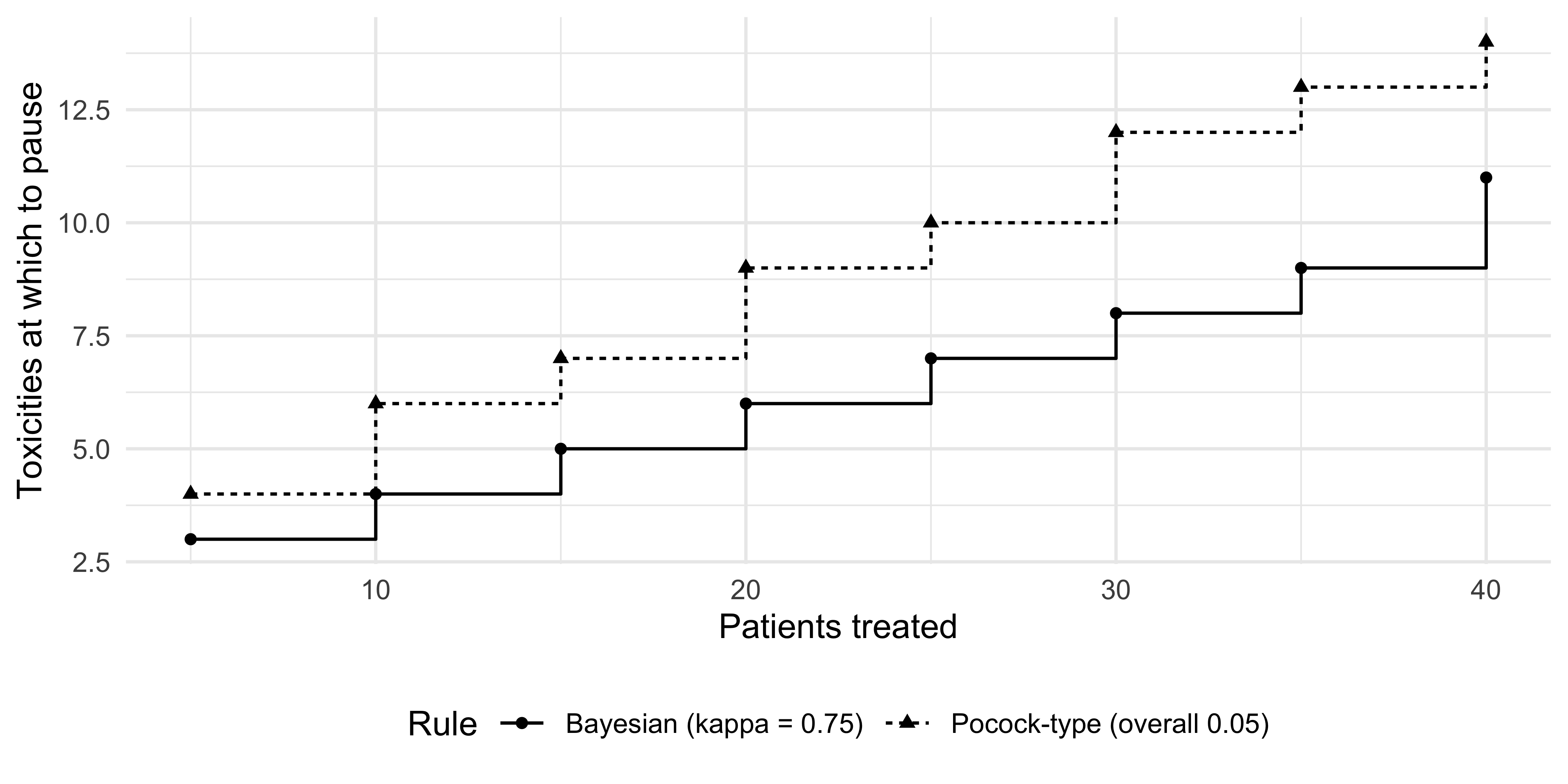
The Bayesian rule stops at 3 of the first 5 patients and 11 of 40. The Pocock-type rule at overall level 0.05 requires 4 of the first 5, and 14 of 40. There is one further fact that the table hides. The Bayes rule’s stopping counts are identical to those of a Pocock-type test whose common nominal level is 0.26: the Bayesian rule is a constant-nominal-level repeated test at these looks, with overall level 0.384 at \(q = 0.2\) (the same calibration, tox_pocock_boundary() at its default). This is not an accident of the example. The posterior probability of exceeding \(\bar q\) is a monotone function of the tail probability under \(\bar q\) at a given \(n\), and the posterior threshold maps to a nominal level that varies slowly with \(n\). The Bayesian rule does not escape the repeated-testing arithmetic; it chooses a point on it, with a threshold, 0.75, that is a statement about how much risk of a false pause the investigators will accept.
Operating characteristics
Both rules are fully described by their boundaries, so their operating characteristics are exact, from a dynamic program over the count of toxicities with no simulation. Table 13.5 gives the probability of stopping early and the expected number of patients enrolled for a range of true toxicity rates.
Table 13.5: Exact operating characteristics of the two toxicity monitoring rules of the previous table: probability of pausing at some look before or at the 40th patient, and expected number of patients treated, by true toxicity rate.
True rate
Bayesian: P(stop)
Bayesian: E[n]
Pocock-type: P(stop)
Pocock-type: E[n]
0.10
0.034
39.1
0.001
40.0
0.15
0.154
36.5
0.008
39.8
0.20
0.384
31.5
0.046
39.1
0.30
0.843
19.7
0.373
33.8
0.40
0.986
12.2
0.827
23.9
At the acceptable rate 0.2 the Bayesian rule pauses the trial with probability 0.384, the Pocock-type rule with probability 0.046. If the true rate is 0.3, an unacceptably high rate by the protocol, they pause with probability 0.843 and 0.373, and the expected enrollment falls from 40 to 19.7 and 33.8. The choice between them is not one of Bayesian against frequentist, since they are members of one family. It is whether, for a safety rule, a pause at a false alarm probability of 0.38 under the boundary rate is acceptable. In many early-phase studies it is. A pause is a review, not an end, enrolled patients are exposed to the unknown, and a monitoring rule with a false pause probability of 0.05 has, in return, a probability of only 0.37 of pausing when the rate is 0.3.
The calibration is deliberate in either direction, and that is the point of a safety rule: it is the asymmetric loss between exposing patients and delaying a good drug that fixes the threshold, so the type I error of a safety boundary is a design choice stated with its consequences, not a number inherited from the efficacy analysis. The operating characteristics belong in the protocol and the DMC charter as the table above does (see Chapter 14 for the report every design carries). A DMC would not follow either table mechanically; the 2006 guidance expects the committee to use judgment, and the boundary is a flag that triggers a review.
Show the R code
d <-rbind(data.frame(n = bnd$n, x = bnd$stop_at, Rule ="Bayesian (kappa = 0.75)"),data.frame(n = poc05$boundary$n, x = poc05$boundary$stop_at, Rule ="Pocock-type (overall 0.05)"))ggplot(d, aes(n, x, linetype = Rule, shape = Rule)) +geom_step() +geom_point() +labs(x ="Patients treated", y ="Toxicities at which to pause") +theme_minimal() +theme(legend.position ="bottom")
Figure 13.1: Stopping counts of the Bayesian toxicity rule and the Pocock-type rule (overall 0.05 at q = 0.2) against patients treated. A trial pauses when the cumulative number of toxicities reaches the count.
13.5 Aggregate safety assessment
A sponsor’s safety review is not one statistic. Four layers sit side by side, and each answers a different question. Blinded pooled review of the whole trial asks whether the overall event rate is higher than expected, without revealing the arms; given credible external information about adverse event rates in comparable untreated patients, Gould and Wang (Gould and Wang 2017) describe Bayesian monitoring for potential excess risk using pooled blinded data (their title calls it the canary in the coal mine). The unblinded DMC review compares arms, with the boundaries and posterior rules of Section 13.2 and Section 13.4. A hierarchical model across adverse event terms, as in Xia, Ma and Carlin (Xia, Ma, and Carlin 2011), shrinks the many rare events toward a common distribution before flagging, in the same way that the gamma-Poisson shrinker does for spontaneous reports. And a false discovery rate flag, such as the double FDR of Mehrotra and Adewale (Mehrotra and Adewale 2012), then limits the expected false-discovery proportion among the flagged terms. Their procedure groups adverse events by body system, whereas Section 10.4.5 defines FDR and illustrates the ordinary Benjamini-Hochberg procedure.
Outside the trial, surveillance of marketed products and vaccines is sequential in the Wald sense. Kulldorff and colleagues (Kulldorff et al. 2011) proposed a maximized sequential probability ratio test for drug and vaccine safety surveillance. With a Poisson count \(c\) of events against an expected count \(\mu_0\) under no excess risk, the statistic is the log likelihood ratio maximized over relative risks above one, \(c\log(c/\mu_0) - (c-\mu_0)\) when \(c > \mu_0\), and a signal is declared when it crosses a critical value that has been calibrated for the planned surveillance. It is the likelihood-ratio machinery of Chapter 12 with a fixed alternative replaced by its maximum, so it needs a critical value from a calibration rather than the \(1/\alpha\) of an e-value. Which of these layers is a trigger for action, and which only a hypothesis for review, is a decision for the safety plan to state, and the regulator will ask for it (Section 13.7).
13.6 Connecting the two views
The toxicity rule is a posterior probability monitor, so it inherits the properties in Section 13.2: its overall false alarm probability is a computed number for the stated schedule and is not guaranteed for looks off the schedule. An e-value version of the same boundary would instead use the likelihood ratio of a binomial alternative against \(\bar q\). It would be valid at any look, including a fifth unscheduled one when a competing trial reads out or a serious event is reported. That is what Chapter 12 argued for DMCs in general, and safety is where its case is strongest, since the schedule of a DMC is almost never exactly the one in the charter. The price, again, is a larger sample at a given power. Which to use is a question of what the charter promises. A rule with a stated boundary at planned looks and a stated false pause probability fits a phase II toxicity review. An e-value threshold is the better statement for a long-running surveillance program or for a pooled monitoring of several trials of one drug, in which the number of looks cannot be fixed.
13.7 What the regulator will ask
Which safety events are monitored, and who sees unblinded data. The IND safety reporting guidance and the DMC guidance ask for a plan, and the plan must say who reviews aggregate data and how.
Which statistical rule is used, and whether it is a trigger for review or an automatic stop. Neither guidance prescribes a rule, and a Bayesian boundary is acceptable on the same terms as a frequentist one: prespecified, with operating characteristics that are reported.
What the false alarm probability and the power are, under the stated schedule and, for a continuous monitor, under looks off the schedule.
How signals from outside the trial (spontaneous reports, other trials of the same drug, the class) enter the review. A shrinkage screen is a hypothesis generator, and it is not a basis for a safety report by itself.
For an event that triggers 21 CFR 312.32, the clock. For an unexpected fatal or life-threatening suspected adverse reaction that is interpretable as a single case, the 7-day limit runs from the sponsor’s initial receipt of the information, whereas the 15-day limit for other potential serious risks runs from the date the sponsor determines that the information qualifies for reporting (21 CFR 312.32(c)). For events that need more than one occurrence or an aggregate analysis to establish a causal relationship, the sponsor makes the determination once it has evidence that the aggregate analysis meets the reporting criterion, and must then report as soon as possible. No monitoring rule shortens these limits or lengthens them (U.S. Food and Drug Administration 2025, sec. VIII).
Key points
Safety evidence accumulates, and the natural analysis is cumulative. The rofecoxib trials had pooled to a relative risk of about 2.3 for myocardial infarction by the end of 2000, and the pooled posterior probability of harm was above 0.91 even under a skeptical prior with standard deviation 0.2 on the log scale.
A \(p\)-value measures how unusual the observed or more extreme data would be under the specified null model. A posterior says how large it probably is and how probable a harm of a given size is, which is what a benefit-risk decision uses. The decision itself needs the benefit side, as in the inequality of this chapter.
Continuous monitoring has two statistics. The posterior probability is coherent under any stopping rule but its false alarm rate is not controlled (about 0.23 over 60 monthly looks at a threshold of 0.95 in the simulation). The Bayes factor read as an e-value is controlled by Ville’s inequality at any look (about 0.02 against a bound of 0.05 for the harm-only factor).
Empirical Bayes shrinkage, the gamma-Poisson shrinker, ranks spontaneous-report signals by evidence as well as by size. A raw ratio of 20 on one report is not a signal; a ratio of 4 on 40 reports is.
A Bayesian toxicity stopping rule is a table of counts. Its operating characteristics are exact (at a true rate of 0.2 it pauses with probability 0.384, and at 0.3 expected enrollment is 19.7 of 40), and it is a constant-nominal-level repeated test, the same family as the Pocock-type rule it is compared with.
No guidance prescribes a statistical stopping rule for safety. 21 CFR 312.32 is a requirement about what to report and when; the DMC and IND safety guidances recommend how to monitor.
NoteDiscussion questions
A sponsor says that the VIGOR excess was explained by naproxen. What data would distinguish that account from harm by rofecoxib, and what Bayes factor would you want to see before accepting it?
A DMC charter fixes a toxicity boundary at 5-patient looks. A serious event occurs between looks. What does the boundary table allow, and what would an e-value boundary have allowed?
A drug-event pair has 3 reports against an expected 0.5, a raw ratio of 6, and an EB05 of 0.72. A clinician says it is a “known” effect. What does the screen say and what does it not say?
The Bayesian toxicity rule pauses a null-rate trial with probability 0.38. Argue for and against a Pocock-type rule at 0.05 for a first-in-human oncology study and for a trial of a vaccine in healthy volunteers.
NoteExercises
Verify the end-2000 rows of Table 13.1. Show that with a \(N(0, s_0^2)\) prior and a normal likelihood with standard error \(0.323\) the posterior is normal with precision \(1/0.323^2 + 1/s_0^2\).
In Equation 13.1 take \(r_0 = 0.01\) per year, \(g = 0.01\) per year and \(d_G / d_M = 0.3\). For which values of \(\mathbb{E}[RR]\) is rofecoxib preferred? (Answer: below 1.3.)
Show that the marginal distribution of \(n\) under a \(\mathrm{Gamma}(\alpha, \beta)\) prior on \(\lambda\) and \(n \sim \mathrm{Poisson}(\lambda E)\) is negative binomial with size \(\alpha\) and success probability \(\beta/(\beta + E)\).
Derive the posterior weight on each gamma component in the shrinker and reproduce the third row of Table 13.3.
Use safety_bf_monitor() with looks = 60 and different pp_threshold values to find the threshold at which the posterior probability rule has a false alarm probability of 0.05. The function simulates null paths only, so to compare the sample size needed to alarm when the true relative risk is 1.5, extend the simulator by adding drift \(\log(1.5)\) to the information-time paths and recording the first crossing of the threshold.
Using tox_bayes_boundary() and tox_oc(), find the smallest threshold \(\kappa\) for which the Bayesian rule’s probability of pausing at \(q = 0.2\) is at most 0.05 (exactly 0.05 is not attainable with discrete boundaries, so report the adjacent attainable values), and compare the boundary with the third column of Table 13.4.
Bate, A., M. Lindquist, I. R. Edwards, S. Olsson, R. Orre, A. Lansner, and R. M. De Freitas. 1998. “A Bayesian Neural Network Method for Adverse Drug Reaction Signal Generation.”European Journal of Clinical Pharmacology 54 (4): 315–21. https://doi.org/10.1007/s002280050466.
Berry, Scott M., and Donald A. Berry. 2004. “Accounting for Multiplicities in Assessing Drug Safety: A Three-Level Hierarchical Mixture Model.”Biometrics 60 (2): 418–26. https://doi.org/10.1111/j.0006-341X.2004.00186.x.
Bombardier, Claire, Loren Laine, Alise Reicin, et al. 2000. “Comparison of Upper Gastrointestinal Toxicity of Rofecoxib and Naproxen in Patients with Rheumatoid Arthritis.”New England Journal of Medicine 343 (21): 1520–28. https://doi.org/10.1056/NEJM200011233432103.
Bresalier, Robert S., Robert S. Sandler, Hui Quan, et al. 2005. “Cardiovascular Events Associated with Rofecoxib in a Colorectal Adenoma Chemoprevention Trial.”New England Journal of Medicine 352 (11): 1092–102. https://doi.org/10.1056/NEJMoa050493.
Curfman, Gregory D., Stephen Morrissey, and Jeffrey M. Drazen. 2005. “Expression of Concern.”New England Journal of Medicine 353 (26): 2813–14. https://doi.org/10.1056/NEJMe058314.
DuMouchel, William. 1999. “Bayesian Data Mining in Large Frequency Tables, with an Application to the FDA Spontaneous Reporting System.”The American Statistician 53 (3): 177–90. https://doi.org/10.1080/00031305.1999.10474456.
Evans, Stephen J. W., Patrick C. Waller, and Susan Davis. 2001. “Use of Proportional Reporting Ratios (PRRs) for Signal Generation from Spontaneous Adverse Drug Reaction Reports.”Pharmacoepidemiology and Drug Safety 10 (6): 483–86. https://doi.org/10.1002/pds.677.
Gould, A. Lawrence, and William B. Wang. 2017. “Monitoring Potential Adverse Event Rate Differences Using Data from Blinded Trials: The Canary in the Coal Mine.”Statistics in Medicine 36 (1): 92–104. https://doi.org/10.1002/sim.7129.
Ivanova, Anastasia, Bahjat F. Qaqish, and Michael J. Schell. 2005. “Continuous Toxicity Monitoring in Phase II Trials in Oncology.”Biometrics 61 (2): 540–45. https://doi.org/10.1111/j.1541-0420.2005.00311.x.
Jüni, Peter, Linda Nartey, Stephan Reichenbach, Rebekka Sterchi, Paul A. Dieppe, and Matthias Egger. 2004. “Risk of Cardiovascular Events and Rofecoxib: Cumulative Meta-Analysis.”The Lancet 364 (9450): 2021–29. https://doi.org/10.1016/S0140-6736(04)17514-4.
Kulldorff, Martin, Robert L. Davis, Margarette Kolczak, Edwin Lewis, Tracy Lieu, and Richard Platt. 2011. “A Maximized Sequential Probability Ratio Test for Drug and Vaccine Safety Surveillance.”Sequential Analysis 30 (1): 58–78. https://doi.org/10.1080/07474946.2011.539924.
Mehrotra, Devan V., and Adeniyi J. Adewale. 2012. “Flagging Clinical Adverse Experiences: Reducing False Discoveries Without Materially Compromising Power for Detecting True Signals.”Statistics in Medicine 31 (18): 1918–30. https://doi.org/10.1002/sim.5310.
Pocock, Stuart J. 1977. “Group Sequential Methods in the Design and Analysis of Clinical Trials.”Biometrika 64 (2): 191–99.
Puijenbroek, Eugene P. van, Andrew Bate, Hubert G. M. Leufkens, Marie Lindquist, Roland Orre, and Antoine C. G. Egberts. 2002. “A Comparison of Measures of Disproportionality for Signal Detection in Spontaneous Reporting Systems for Adverse Drug Reactions.”Pharmacoepidemiology and Drug Safety 11 (1): 3–10. https://doi.org/10.1002/pds.668.
Rothman, Kenneth J., Stephan Lanes, and Susan T. Sacks. 2004. “The Reporting Odds Ratio and Its Advantages over the Proportional Reporting Ratio.”Pharmacoepidemiology and Drug Safety 13 (8): 519–23. https://doi.org/10.1002/pds.1001.
Szarfman, Ana, Stella G. Machado, and Robert T. O’Neill. 2002. “Use of Screening Algorithms and Computer Systems to Efficiently Signal Higher-Than-Expected Combinations of Drugs and Events in the US FDA’s Spontaneous Reports Database.”Drug Safety 25 (6): 381–92. https://doi.org/10.2165/00002018-200225060-00001.
Thall, Peter F., Richard M. Simon, and Elihu H. Estey. 1995. “Bayesian Sequential Monitoring Designs for Single-Arm Clinical Trials with Multiple Outcomes.”Statistics in Medicine 14 (4): 357–79. https://doi.org/10.1002/sim.4780140404.
———. 1996. “New Statistical Strategy for Monitoring Safety and Efficacy in Single-Arm Clinical Trials.”Journal of Clinical Oncology 14 (1): 296–303. https://doi.org/10.1200/jco.1996.14.1.296.
U.S. Food and Drug Administration. 2006. “Guidance for Clinical Trial Sponsors: Establishment and Operation of Clinical Trial Data Monitoring Committees.”https://www.fda.gov/media/75398/download.
———. 2025. “Sponsor Responsibilities – Safety Reporting Requirements and Safety Assessment for IND and Bioavailability/Bioequivalence Studies: Guidance for Industry.” Center for Drug Evaluation; Research; Center for Biologics Evaluation; Research. https://www.fda.gov/media/150356/download.
Ville, Jean. 1939. Étude Critique de La Notion de Collectif. Monographies Des Probabilités 3. Paris: Gauthier-Villars.
Xia, H. Amy, Haijun Ma, and Bradley P. Carlin. 2011. “Bayesian Hierarchical Modeling for Detecting Safety Signals in Clinical Trials.”Journal of Biopharmaceutical Statistics 21 (5): 1006–29. https://doi.org/10.1080/10543406.2010.520181.
Zorych, Ivan, David Madigan, Patrick Ryan, and Andrew Bate. 2013. “Disproportionality Methods for Pharmacovigilance in Longitudinal Observational Databases.”Statistical Methods in Medical Research 22 (1): 39–56. https://doi.org/10.1177/0962280211403602.