5  Randomization From the Ground Up

Every trial in this book rests on one act that is so familiar it is easy to overlook: a patient is assigned to a treatment by chance. The rest of the apparatus, the p-value of Chapter 4, the posterior probabilities of Chapter 6, the interim looks of Chapter 11, all assume that the two groups being compared differ only because of the treatment, and by luck of the draw. This chapter explains why that assumption is credible when the assignment is random and not credible otherwise, how randomization is carried out in practice, what it means for a sequence to be random, and what a trialist must do after randomization to keep what it bought. We start with a doctor who chooses patients, because the failure of that arrangement is the reason the rest of the chapter exists.

The standard practice comes first. Everything here, simple and blocked randomization, stratification, minimization, concealment, blinding, intention to treat, is what a protocol written today for a regulator already contains. Response-adaptive randomization, where the allocation probabilities change as data accumulate, is a departure from this standard and is taken up in Chapter 16. A reader who knows the standard well can go straight to the sections on randomness and on why a Bayesian still randomizes.

ImportantRegulatory anchor

ICH E9, Statistical Principles for Clinical Trials (Step 4, February 1998). Section 2.3.2 on randomization: “Randomisation introduces a deliberate element of chance into the assignment of treatments to subjects in a clinical trial,” and it “also tends to produce treatment groups in which the distributions of prognostic factors, known and unknown, are similar.” Section 2.3.1 on blinding defines the double-blind trial as one in which neither the subject nor any of the investigator or sponsor staff involved in treatment or evaluation are aware of the treatment received. Section 5.2.1 says that the intention-to-treat principle implies that the primary analysis should include all randomized subjects and says that preserving the initial randomization in analysis is important in preventing bias.

ICH E9(R1), Addendum on Estimands and Sensitivity Analysis (Step 4, November 2019). Requires the treatment effect of interest to be defined, before the trial, as an estimand, with an explicit strategy for each intercurrent event (treatment discontinuation, rescue medication, death).

ICH E8(R1), General Considerations for Clinical Studies (Step 4, October 2021). Lists randomization, blinding or masking, and control of confounding among the approaches to minimize bias, and says that randomized studies play a central role in drug development because they can better control biases.

21 CFR 314.126(b)(4) and (b)(5). An adequate and well-controlled investigation must use a method of assigning patients to treatment that minimizes bias and ensures comparability of the groups on pertinent variables such as age, sex and severity of disease, and must take adequate measures to minimize bias on the part of subjects, observers and analysts. See Chapter 3 for the map of these documents.

5.1 Why allocate by chance

The counterfactual problem

Suppose a new drug is given to some patients and not to others. For any one patient we see one outcome. We never see what would have happened to the same patient under the other treatment. Write \(Y(1)\) for the outcome a patient would have if treated and \(Y(0)\) for the outcome if not. The treatment effect for that patient is \(Y(1) - Y(0)\), and we can never observe both terms. This is the fundamental problem of causal inference in the potential outcomes language of Rubin (Rubin 1974), and every trial design is a way of getting around it.

What we can do is compare groups. Let \(D = 1\) mean “was assigned to the drug” and \(D = 0\) mean “was not”, and assume complete adherence in this opening example (the intention-to-treat section below separates assignment from receipt). The difference in average observed outcomes between the groups can be written as

\[ \begin{aligned} \underbrace{\mathbb{E}[Y \mid D=1] - \mathbb{E}[Y \mid D=0]}_{\text{what the trial shows}} \;=\;& \underbrace{\mathbb{E}[Y(1) - Y(0) \mid D=1]}_{\text{effect on those who were treated}}\\ &+\; \underbrace{\mathbb{E}[Y(0) \mid D=1] - \mathbb{E}[Y(0) \mid D=0]}_{\text{selection bias}} . \end{aligned} \tag{5.1}\]

The last term asks how different the two groups were before the drug did anything: what would have happened to the treated patients had they not been treated, compared with what did happen to the untreated. If the groups were chosen in a way that depends on prognosis, the term is not zero, and the observed difference mixes the effect of the drug with the effect of the choice. If the assignment is made by a coin that ignores everything about the patient, then the treated and untreated groups are two random samples from the same population, the selection term is zero on average, and the difference in observed means estimates the average effect of the drug. That is the whole argument, and it needs no assumption about which patient characteristics matter. R. A. Fisher made it central to experimental design (Fisher 1935), and it is the reason the regulation asks for a method of assignment that minimizes bias.

Confounding by indication: a doctor picks the patients

The commonest way for the selection term to be nonzero in medicine is confounding by indication: the reasons a doctor chooses a treatment are themselves related to the outcome. A physician who believes a new drug is promising may offer it to patients who seem strong enough to benefit and keep the old treatment for the frail. No bad faith is required. The physician is doing what a physician is supposed to do, using judgment on behalf of each patient, and that is exactly what ruins the comparison.

We can see the damage in a simulation. Each patient has a hidden health score \(h\) that the doctor senses but that is not recorded. Healthier patients are more likely to recover whatever they receive. The new drug truly adds 10 percentage points to the probability of recovery. In the first scheme the doctor offers the drug with probability that rises with \(h\). In the second, a coin decides. Each trial has 400 patients and we run 1,000 trials of each kind.

set.seed(2026)
sim <- function(a) as.data.frame(t(replicate(1000, sim_confounded_trial(400, assign = a))))
doc <- sim("doctor"); coin <- sim("coin")
d <- rbind(data.frame(scheme = "doctor chooses", est = doc$naive),
           data.frame(scheme = "coin chooses", est = coin$naive))
ggplot(d, aes(est, fill = scheme)) + geom_histogram(bins = 60, alpha = 0.8, position = "identity") +
  geom_vline(xintercept = 0.10, linetype = 2) + scale_fill_manual(values = c("#2a9d8f", "#e08a2c")) +
  labs(x = "observed difference in recovery rate (drug minus control)", y = "trials", fill = NULL) +
  theme_minimal() + theme(legend.position = "top")

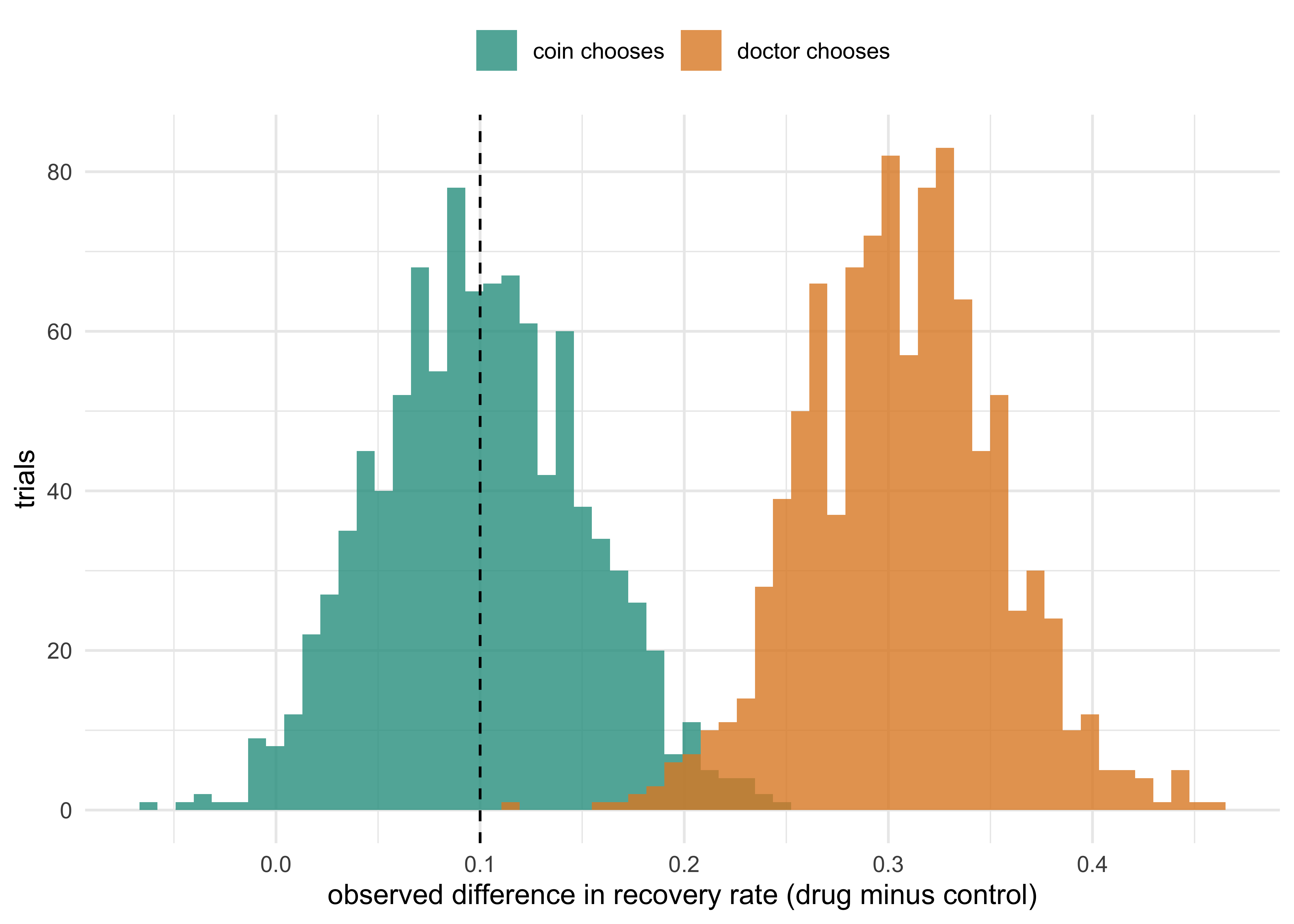
Figure 5.1: Estimated effect of a drug that truly adds 10 percentage points to recovery, in 1,000 simulated trials of 400 patients. When a doctor chooses who gets the drug (orange) the healthier patients end up on it and the estimates are centred far above the truth. When a coin chooses (teal) they are centred on the truth. The dashed line marks the true effect.

The doctor’s trials do not scatter around the truth. They scatter around roughly three times the truth (the mean estimate is 0.31), and in 100 percent of the 1,000 trials the drug looks better than it is. The reason is in the health gap: the patients given the drug were 1.06 standard deviations healthier than the patients who were not, and nothing in the recorded outcome tells you so. The standard error of the estimate is about the same in the two schemes (0.048 for the doctor, 0.05 for the coin), so a larger trial would not help. It would only make the wrong answer more convincing.

A natural reaction is that the analyst should adjust for health. That works when health has been measured well. Suppose we do record \(h\) and compare treated and untreated patients within five bands of \(h\). Then the estimate of the doctor-chosen trials, in the chunk below, falls from about 0.31 to about 0.12, much closer to the truth, but still not equal to it, because patients within a band still differ and the doctor’s choice depends on \(h\) itself.

set.seed(8)
r <- t(replicate(300, sim_adjusted_vs_naive(2000)))
knitr::kable(data.frame(Estimate = c("Truth", "Naive", "Stratified on health"), Value = c(0.100, mean(r[, "naive"]), mean(r[, "adjusted"]))), digits = 3, align = "lr")

Estimate	Value
Truth	0.100
Naive	0.306
Stratified on health	0.117

And in real data the doctor’s impression is rarely a clean recorded number. The coin needs no such measurement. It balances health as recorded, health as sensed and health that nobody has thought of, which is the content of the sentence in ICH E9 about prognostic factors “known and unknown”.

5.2 What goes wrong without it

The simulation is a cartoon. The history of medicine supplies the real thing, in four recurring forms.

Historical controls. The new treatment is given to patients now and compared with patients treated in the past. Patients change over time: referral patterns, supportive care, diagnostic criteria and even the way outcomes are recorded move. Sacks, Chalmers and Smith reviewed studies of six therapies, each of which had been studied with both randomized and historical controls, and found that the historically controlled studies were much more likely to report the new therapy as better than the randomized ones (Sacks, Chalmers, and Smith 1982). The pattern, that the nonrandomized comparison finds benefit more often than the randomized one, is what Equation 5.1 predicts when the investigator’s access to patients and the trend over time both favor the new treatment. FDA’s regulation recognizes the problem: 21 CFR 314.126(b)(2)(v) lists the historical (external) control as a type of control that is considered, and the Substantial Evidence draft guidance (June 2026) notes that differences between groups are a particular concern “because of the lack of randomized treatment assignment”. We return to when external controls are nonetheless useful, and how to borrow from them, in Chapter 19.

Alternation and other predictable schemes. Giving every other patient the new drug looks like a fair procedure. It is not, because the next assignment is known to the person who decides whether the next patient is eligible. A clinician who knows that the next patient will receive the experimental drug can steer a frail patient away (or toward it) by deciding that the patient is not quite eligible, or by delaying enrollment by a day. The scheme is not random, and it is not concealed. The Medical Research Council’s 1948 streptomycin trial solved this problem with concealed allocation (see “In practice” below).

Unconcealed allocation. Even a perfectly random list is useless if the enrolling clinician can read it. Schulz and colleagues examined 250 controlled trials from 33 meta-analyses in pregnancy and childbirth and found that trials with inadequately concealed allocation reported odds ratios that were exaggerated, on average, by about 41 percent, and trials whose concealment was unclearly reported by about 30 percent, compared with trials with adequate concealment (Schulz et al. 1995). These are averages over one body of trials, an association and not a randomized comparison of concealment methods. A separate paper from the same group describes the many ways clinicians have been seen to subvert allocation schedules: holding envelopes up to bright lights and opening several envelopes at once, among others (Schulz 1995). These are results about the process by which patients are assigned, not about the mathematics of randomness. We return to concealment in a later section.

Self-selection by patients. If patients decide which arm to join, the decision is again related to prognosis. A trial in which sicker patients seek the experimental treatment, or healthier, more motivated patients adhere to the offered regimen, compares people who differ in more than the treatment. The Women’s Health Initiative is the instructive example, because its randomized result reversed an observational finding about hormone therapy (see “In practice” below).

The first lesson of this section is that these failures are failures of assignment, not of analysis. No statistical adjustment applied afterward can repair an assignment mechanism that depended on unrecorded information. The second is that randomization is only as good as its concealment: a random list that the investigator can see is a way of choosing patients with extra steps. The two together are the content of the phrase “adequate and well-controlled”.

5.3 Methods of randomization

All the methods below assign each patient to treatment or control with some chance. They differ in how they use constraints to avoid unlucky draws. In this section we assume two arms with 1:1 allocation. Rosenberger and Lachin give a full treatment of the theory (Rosenberger and Lachin 2016); ICH E9 (section 2.3.2) advises that the block size be kept unknown to the investigators and that the randomization schedule be filed securely by the sponsor; the specification should be written so that the schedule is reproducible.

Simple randomization

The simplest method assigns each patient by a fair coin, independently of every other patient. Its strength is that it is unpredictable: knowing all previous assignments tells you nothing about the next one. Its weakness is that, in a small trial, chance may give unequal arm sizes and unequal covariate distributions. With \(n = 40\) patients, the number in the treatment arm has standard deviation \(\sqrt{40}/2 \approx 3.2\), so a split of 15 and 25 is not rare. The loss is not catastrophic (it costs a little efficiency), but the covariate imbalance is more serious, as we will see.

Permuted block randomization

Permuted block randomization fixes the arm sizes at intervals. Patients are grouped in consecutive blocks of, say, four. In each block, two get the drug and two get control, in a random order (there are six possible orders, each equally likely). After every block the arms are exactly balanced in size, and at any moment the imbalance cannot exceed half a block. This also protects the trial against a time trend: if the standard of care slowly improves, both arms have patients from each period. (Zelen (Zelen 1974) reviews stratified permuted blocks; Efron’s biased coin (Efron 1971) and Wei’s adaptive version (Wei 1978) are early alternatives.)

The price is predictability. If the block length is fixed at four and the investigator knows it, then after the first three patients of a block have been assigned, the fourth assignment is always determined. Suppose the first three patients were assigned drug, drug, control. The fourth must be control. A clinician who can see past assignments (open-label trials, or trials with unmasked packaging) can use this to select patients. The standard remedy is to vary the block length at random (for example, blocks of 4 and 6, drawn at random) and to keep the block sizes out of the protocol text and in the unblinded randomization plan.

Stratified randomization

If a prognostic factor is known to matter, such as disease stage, prior treatment or study center, we can balance it by design. We run a separate permuted-block list inside each stratum, the combination of levels of the factors. Every stratum then has near-equal arm sizes. ICH E9 (section 5.7) asks that the factors used to stratify the randomization be accounted for in the analysis. Stratification has a ceiling: with \(k\) binary factors there are \(2^k\) strata, and each stratum has its own incomplete block at the end of enrollment. With 20 patients percenter and four factors, most blocks are unfinished and the stratification has bought little. A good rule is to stratify on few factors (two or three) that are strongly prognostic, and to analyze the primary endpoint adjusting for those same factors, a point we come back to below. Kernan and colleagues review the method and its practical limits (Kernan et al. 1999).

Minimization

Minimization is the method for small trials with many prognostic factors. Taves (Taves 1974) and, independently, Pocock and Simon (Pocock and Simon 1975) proposed assigning each new patient in a way that depends on what has happened so far: look at the patient’s levels of each factor, count how many earlier patients with those same levels are in each arm, and assign the new patient to the arm that makes the total imbalance smaller. In its deterministic form it is not random at all, and the next assignment can be predicted by anyone who knows the current counts. Pocock and Simon therefore proposed to assign to the preferred arm with a probability \(p\) larger than a half (0.8 is a common choice), and to a fair coin when the arms tie. The package function assign_minimization implements exactly this. The Pocock-Simon method balances the margins of each factor (the number of women in each arm, the number of patients over 65 in each arm) but not necessarily the combinations. Reviews of the method (Scott et al. 2002) stress that the analysis should include the minimization factors as covariates, because in a minimized trial the assignment is not independent of those factors.

Seeing the difference

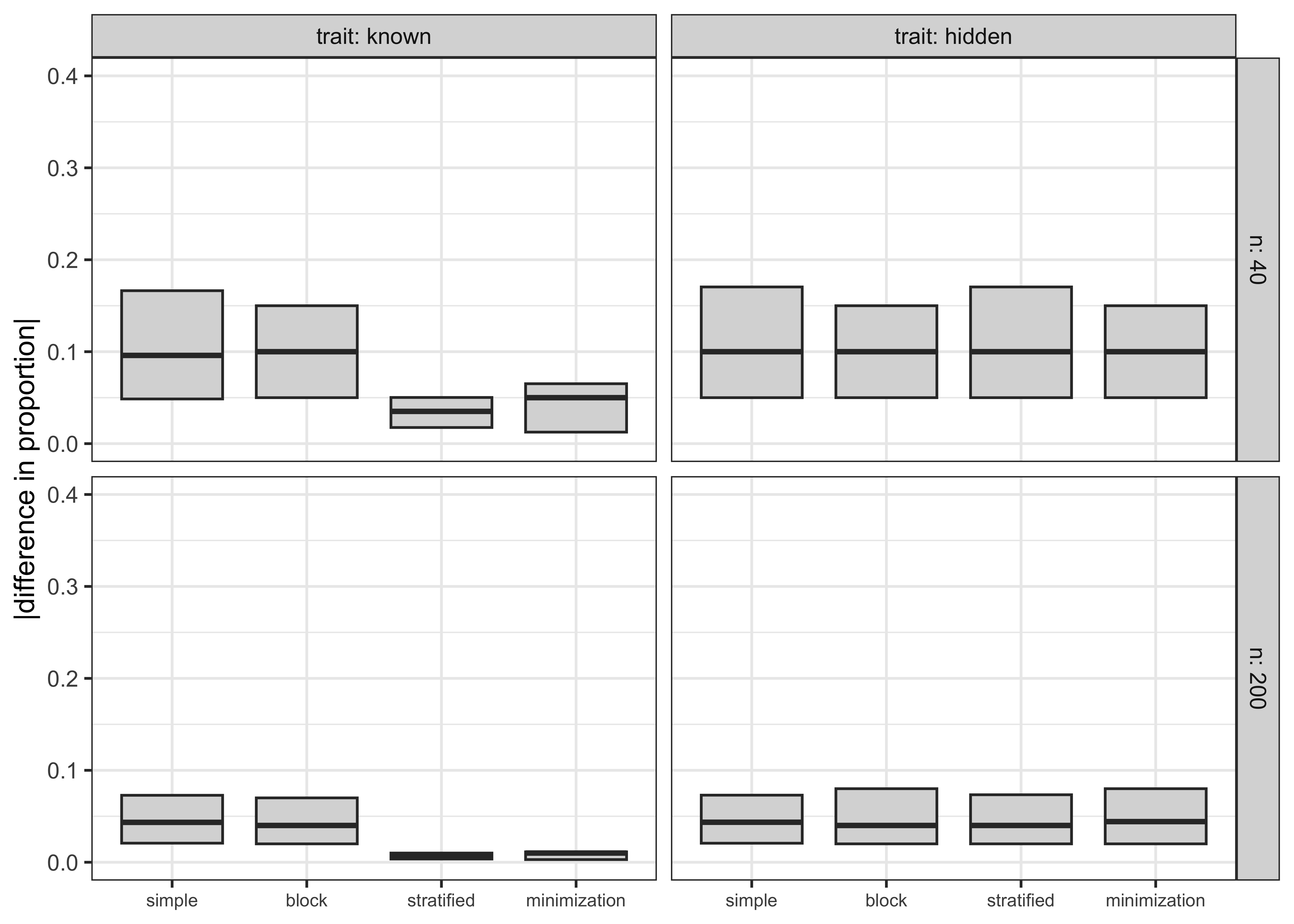
Each method has a different effect on how balanced the arms are. We simulate trials of 40 and 200 patients with three binary traits: two known and used in stratification and minimization (for example, sex and age above 65, with the second being less common) and one unmeasured (a hidden trait with prevalence 0.3 that nobody recorded). For each method we compute the absolute difference between arms in the proportion of patients who have the second known trait, and in the proportion who have the hidden trait.

set.seed(11)
one <- function(n) {
  sex <- rbinom(n, 1, 0.5); old <- rbinom(n, 1, 0.3); hid <- rbinom(n, 1, 0.3)
  arms <- list(simple = assign_simple(n), block = assign_block(n, 4),
               stratified = assign_stratified(sex * 2 + old, 4),
               minimization = assign_minimization(cbind(sex, old)))
  sapply(arms, function(a) c(known = covariate_imbalance(a, old), hidden = covariate_imbalance(a, hid)))
}
res <- do.call(rbind, lapply(c(40, 200), function(n)
  cbind(n = n, as.data.frame(as.table(replicate(1000, one(n)))))))
names(res) <- c("n", "trait", "method", "rep", "gap")
imb <- aggregate(gap ~ n + trait + method, res, mean)
g <- function(n, m, t = "known") imb$gap[imb$n == n & imb$method == m & imb$trait == t]
q95 <- quantile(res$gap[res$n == 40 & res$trait == "known" & res$method == "simple"], 0.95)
ggplot(res, aes(method, gap)) + geom_boxplot(outlier.shape = NA, coef = 0, fill = "grey85") +
  facet_grid(n ~ trait, labeller = label_both) + coord_cartesian(ylim = c(0, 0.4)) +
  labs(x = NULL, y = "|difference in proportion|") + theme_bw() +
  theme(axis.text.x = element_text(size = 7))

Figure 5.2: Imbalance between arms in the proportion with a binary trait, 1,000 simulated trials per method. Left: the trait is known and used by the method (stratified blocks of 4, or Pocock-Simon minimization). Right: the trait is hidden and nobody balances it. Stratification and minimization remove the imbalance in the known trait and do nothing for the hidden one, which is as imbalanced as under simple randomization.

Three things stand out. First, at \(n = 40\) the average gap in the known trait under simple randomization is about 0.12, and in one trial in twenty it is larger than about 0.3. That is imbalance big enough to matter if the trait is prognostic. At \(n = 200\) it falls by a factor of \(\sqrt{5}\), to about 0.05. Second, stratified blocks and minimization cut the imbalance in the known trait to a fraction of that (at \(n = 40\), 0.04 for stratified blocks and 0.04 for minimization; at \(n = 200\), 0.01 and 0.01). Third, nothing helps the hidden trait: its imbalance is the same under all four methods, as large as under simple randomization. Randomization does not guarantee balance in any single trial. What it guarantees is that the imbalance is due to chance, with a known distribution, and that this distribution is what the confidence interval and the p-value account for. This is why a randomized trial can be analyzed honestly without balance, and a confounded one cannot.

NoteTechnical note: why blocks do nothing for covariate imbalance

A permuted block makes the number of patients in each arm equal. It says nothing about which patients. For a covariate \(x_i \in \{0,1\}\) unrelated to the order of enrollment, the assignment within a block is a random permutation, so each patient’s arm is still a fair coin independent of \(x_i\) and the covariate imbalance has the same distribution as under simple randomization apart from a small finite-population correction. The simulation shows the effect: the “block” boxplots match the “simple” ones. Blocks help with arm size and with time trends. For covariates, stratification inside blocks, or minimization, is needed.

How the schedule is actually made

In a trial that uses an interactive response technology (IRT, formerly IVRS and IWRS), the investigator does not see a list. The site enters the patient’s stratification factors into a web or phone system, and the system returns a kit or bottle number. Behind it is a randomization schedule produced by an unblinded statistician (or the vendor) before the trial starts, from a pseudo-random number generator and a stored seed. The schedule is a table: stratum, sequence number within the stratum, treatment, kit number. It is generated once, checked for balance and validated, and then locked. The protocol should state the allocation method, the strata and the access controls, so that site staff, monitors and the blinded statistical team cannot see the schedule. A separate restricted randomization specification should record the block sizes, generator settings and seed, so that the schedule can be reproduced by an auditor (ICH E9 advises keeping details that would let assignments be predicted, block length in particular, out of the protocol).

strata <- rep(c("stage II", "stage III", "stage IV"), each = 30)
arm <- assign_stratified(strata, sizes = c(4, 6), seed = 20261108)     # seed recorded in the randomization specification
sched <- data.frame(stratum = strata, seq = ave(arm, strata, FUN = seq_along),
                    arm = ifelse(arm == 1, "drug", "control"))
set.seed(1); sched$kit <- sample(1001:(1000 + nrow(sched)))           # kit number reveals nothing
knitr::kable(head(sched, 8), col.names = c("Stratum", "Sequence in stratum", "Arm", "Kit number"), align = "lrlr")

Stratum	Sequence in stratum	Arm	Kit number
stage II	1	control	1068
stage II	2	control	1039
stage II	3	drug	1001
stage II	4	drug	1034
stage II	5	control	1043
stage II	6	drug	1014
stage II	7	control	1082
stage II	8	drug	1059

Two properties matter. The schedule is reproducible from the seed, which lets an auditor confirm that nobody altered it. And the site staff see only the kit number the system returns after the patient is irreversibly enrolled, which is what allocation concealment means in practice and which we turn to next.

5.4 Allocation concealment

Randomization has two parts that are easy to confuse. Sequence generation produces the unpredictable list. Allocation concealment keeps that list hidden from the people who decide whether, and when, a patient enters the trial, until the moment the patient is irreversibly enrolled. Concealment is about the time before the assignment. Blinding, which we cover next, is about the time after it. A trial can be concealed and open-label (the patient is randomized by a central system and then sees that they are getting an injection), and in this case the bias of the investigator in selecting patients is prevented but the bias in treatment and assessment is not. A trial cannot be properly blinded without concealment, because an investigator who knows the next assignment already knows the arm.

The practical means are central randomization by IRT, sequentially numbered opaque sealed envelopes (opened only after the patient’s name is written on them and the patient is enrolled), and pharmacy-controlled coded packs. Of these, central telephone or web randomization is the strongest, because it cannot be opened in advance, and is the usual choice in pivotal trials. The evidence summarized earlier (Schulz et al. 1995) shows why: concealment is a property of the process and is something that can be assessed. CONSORT reporting (and the SPIRIT 2025 protocol statement (Chan et al. 2025)) asks authors to say how it was done. Altman and Schulz summarize why and how to conceal allocation (Altman and Schulz 2001).

TipIn the protocol

A concealment paragraph a reviewer can check: “Patients will be randomized centrally through the IRT system after eligibility has been confirmed and informed consent signed. The system returns a kit number only after the patient has been entered. The randomization schedule, block sizes and seed are held by the unblinded statistician at the vendor and are not available to the sponsor’s blinded team, to site staff or to monitors. Block sizes vary at random. Any request to unblind goes through the emergency unblinding procedure of the IRT and is logged.”

5.5 Randomization inference: the test the design justifies

Chapter 4 introduced the permutation test: take the observed outcomes, shuffle the group labels many times, and ask how often a shuffled difference is as large as the observed one. At that point the test was presented as a device. Here we can say what it is for. The randomization test is justified by the design. When treatment was assigned by a known random mechanism, then under the hypothesis that the drug has no effect on any patient (the sharp null: \(Y_i(1) = Y_i(0)\) for every \(i\)), each patient’s outcome would have been the same whatever arm they were assigned to, and the only thing that varied from one possible trial to another was the assignment. The permutation distribution is therefore the exact distribution of the statistic over the possible assignments, computed under the same randomization procedure that was used. It requires no model for the outcome (no normality, no equal variance), and the type I error is controlled by construction. Fisher put this forward in 1935 as the logical basis of significance testing in experiments (Fisher 1935), and the normal-theory z and t tests of Chapter 4 are approximations to it.

The phrase “under the same randomization procedure” is important. Shuffling labels freely is correct if the original assignment was by simple randomization. If it was by permuted blocks, the shuffle should respect the blocks: the possible assignments are only those with two drug and two control in each block. A test that ignores this treats as possible many assignments that the design excluded. We can see what that costs under a time trend. We simulate a null trial of 40 patients, where the drug does nothing but the average outcome drifts upward during enrollment by two standard deviations (a plausible effect if the standard of care changes or the mix of referring centers evolves). We analyze each trial by the one-sided permutation test with a nominal level of 0.025, once unrestricted and once restricted to the blocks.

set.seed(5); n <- 40; R <- 2000
blocks <- split(seq_len(n), rep(seq_len(n / 4), each = 4))
run <- function(scheme) {
  p <- replicate(R, {
    y <- 2 * (seq_len(n) - 1) / n + rnorm(n)                           # drift, no drug effect
    a <- if (scheme == "simple") assign_simple(n) else assign_block(n, 4)
    c(perm_test_arm(y, a, nsim = 500)["p"],
      if (scheme == "block") perm_test_arm(y, a, nsim = 500, restricted_blocks = blocks)["p"] else NA)
  })
  c(unrestricted = mean(p[1, ] <= 0.025), within_blocks = mean(p[2, ] <= 0.025))
}
tab <- data.frame(assignment = c("simple", "block"), rbind(run("simple"), run("block")))
knitr::kable(tab, digits = 3, col.names = c("assignment used", "unrestricted shuffle", "shuffle within blocks"))

Table 5.1: Empirical type I error (one-sided, nominal 0.025) of the permutation test under a time trend and no treatment effect, 2,000 simulated trials of 40 patients per row, 500 permutations each. Monte Carlo standard error is about 0.003.

assignment used	unrestricted shuffle	shuffle within blocks
simple	0.025	NA
block	0.011	0.022

With simple randomization the unrestricted shuffle is the right test, and its error rate (0.025) is close to nominal. With blocks, the unrestricted shuffle treats as possible many assignments the design excluded: with this drift its error rate is 0.011, well below the nominal 0.025 (the Monte Carlo standard error is about 0.003), so the test is conservative and gives away power. The shuffle within blocks gives 0.022, close to nominal; it is the exact test for the design, up to the discreteness of a 40-patient permutation distribution and Monte Carlo error. The lesson for the statistical analysis plan is that the analysis should mirror the randomization, and that factors used in stratification should be in the model for the primary analysis. ICH E9 makes the same point for covariates: the analysis should reflect the stratification used in the design.

The randomization test also answers a question that the normal-theory tests answer only by assumption: what population does the p-value refer to? The patients in a trial are not a random sample from anything. They are the people who consented and were eligible at the participating sites. Randomization inference does not need them to be a sample. It asks only about the patients actually enrolled, and says whether the difference between the arms is larger than the randomization alone would produce. Generalizing to future patients is a separate step that rests on clinical judgment, and it is a step that the p-value does not take.

5.6 What randomness is

So far “random” has meant “by a coin”. For a protocol that is enough. But a trialist who asks what makes a schedule random, and whether a computer generates it properly, is asking a real question. There are two answers, one from information theory and one from geometry, and a practical consequence.

Randomness as incompressibility

Look at two strings of 0s and 1s of the same length. One is 0101010101… repeated. The other was obtained by tossing a coin. We feel the first is not random, because it can be described in a few words: “repeat 01”. The second cannot be described more briefly than by writing it out. Kolmogorov turned this feeling into a definition (Kolmogorov 1965): a string is random if it cannot be described by anything much shorter than the string itself (its complexity is close to its length).

Two facts follow that matter for trials. First, randomness in this sense is a property of a sequence, not of a procedure, and no particular finite sequence can be certified random: Kolmogorov complexity cannot be computed. The best a trialist can do is to apply tests. Second, a sequence produced by a short program (a pseudo-random number generator started from a seed) has low complexity by definition, because the program and the seed describe it. That is not a flaw for a clinical trial, because what matters is that nobody can predict the sequence without the seed. It is why the seed belongs in the sealed randomization specification and is a reason to use a generator of good statistical quality.

NoteTechnical note: complexity, and a compression experiment

Formally, the complexity of a string is the length of the shortest computer program that outputs it. This definition concerns finite strings and program length without restriction. Martin-Löf defined randomness for infinite sequences through effective statistical tests (Martin-Löf 1966), and the equivalence with incompressibility holds for infinite sequences whose prefixes all have high prefix-free complexity, not for the finite-string definition above; Li and Vitányi give the precise theorem (Li and Vitányi 2019).

A crude illustration uses an everyday compressor in place of the shortest program. A compressor finds only some patterns, so its output length is an upper bound on the complexity.

set.seed(7)
coin <- rbinom(2000, 1, 0.5)                                    # fair coin
alternating <- rep(0:1, 1000)                                   # alternation: drug, control, drug, ...
formula_bits <- rand_bits_lcg(2000, seed = 1, a = 75, m = 65537)   # a one-line formula, no obvious pattern
anu <- as.integer(strsplit(trimws(readLines("data/anuqrng.txt", warn = FALSE)[1]), "")[[1]])[1:2000]  # ANU quantum generator
cr <- sapply(list(coin = coin, alternation = alternating, formula = formula_bits, ANU_quantum = anu), compress_ratio)
knitr::kable(data.frame(Sequence = names(cr), `Compressed size / original size` = unname(cr), check.names = FALSE), digits = 3, align = "lr")

Sequence	Compressed size / original size
coin	0.176
alternation	0.012
formula	0.182
ANU_quantum	0.179

The coin sequence compresses to about 0.18 of its size, which is as far as it will go (the floor is 0.125, since each stored character carries one bit and the rest is overhead). The alternation compresses to about 1 percent. The bits of a one-line multiplicative generator (\(x_{k+1} = 75\,x_k \bmod 65537\)) are also not compressed, although a very short program generates them: the compressor does not see the structure, and this is a small demonstration that passing a compression test is not a proof of randomness. The last entry is the first 2,000 bits of a string from the ANU quantum random number generator, which is physically random and compresses as the coin does; a compressor cannot tell it from the one-line formula. A sequence that looks random to a particular test may have a short generator. For clinical use the requirement is therefore practical: a generator with documented statistical quality, a recorded seed, and a schedule that the people who enroll patients cannot see.

Arnold’s measure of randomness

V. I. Arnold proposed a different, geometric, way to judge how random a set of points on a circle looks (Arnol’d 2006). His measure asks whether the points are spread the way independent draws would be spread: evenly spaced points are too regular to be random, and clumped points are too attracted to one another. Applied to a sequence of integers modulo a number, it flags the overly regular ones. For allocation the consequence is practical. A schedule generated by a linear congruential generator with a short period or poor lattice structure fails such tests, and this is a reason to use a modern generator such as the Mersenne Twister (the R default) or PCG64 with a long period, and not to write one’s own.

NoteTechnical note: Arnold’s stochasticity parameter

Arnold’s measure takes \(T\) points on a circle of length \(L\) (Arnol’d 2006). Sort them and let \(x_1,\dots,x_T\) be the gaps between neighbours around the circle, so that \(\sum x_i = L\). His stochasticity parameter is the normalized sum of squared gaps,

\[ s \;=\; T \sum_{i=1}^{T} \left(\frac{x_i}{L}\right)^{2}, \qquad 1 \le s \le T . \tag{5.2}\]

If the points are evenly spaced (“barracks-like”), \(s = 1\), which Arnold calls strong repulsion. If all of them are clustered in one place, \(s = T\), strong attraction. For \(T\) points placed independently and uniformly at random, \(s\) has expected value \(s_1 = 2T/(T+1)\), close to 2 for large \(T\), which he calls the “freedom-loving” value: neither repulsion nor attraction. A sequence of \(T\) integers modulo \(L\) is thus judged by where its \(s\) falls relative to \(s_1\). Values close to 1 mean the points are too evenly spread to be random, values much above \(s_1\) mean they clump.

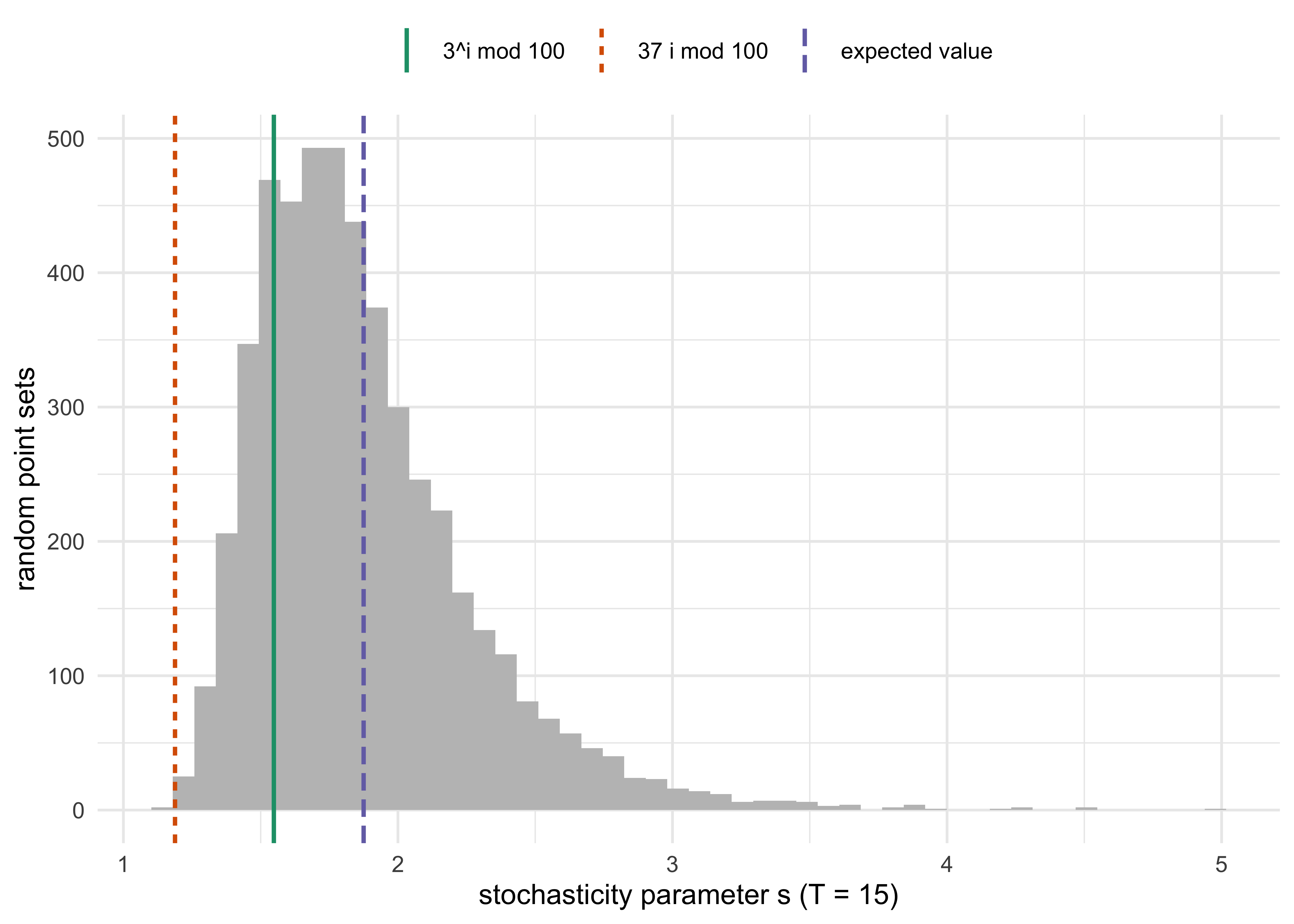
Here is the example in R: 15 residues modulo 100 from the formula \(3^i\), from the formula \(37i\), and from the random number generator, and then the distribution of \(s\) over many random sequences.

set.seed(3); T <- 15
seq_a <- (3^(1:T)) %% 100; seq_b <- (37 * (1:T)) %% 100
sa <- arnold_stochasticity(seq_a, 100); sb <- arnold_stochasticity(seq_b, 100)
sc <- arnold_stochasticity(sample(1:100, T, replace = TRUE), 100)
draws <- replicate(5000, arnold_stochasticity(sample.int(1e6, T, replace = TRUE), 1e6)["S"])
ci <- quantile(draws, c(0.025, 0.975))
marks <- data.frame(s = c(sa["expected"], sa["S"], sb["S"]),
                    what = c("expected value", "3^i mod 100", "37 i mod 100"))
ggplot(data.frame(s = draws), aes(s)) + geom_histogram(bins = 50, fill = "grey75") +
  geom_vline(data = marks, aes(xintercept = s, colour = what, linetype = what), linewidth = 0.8) +
  scale_colour_brewer(palette = "Dark2") +
  labs(x = "stochasticity parameter s (T = 15)", y = "random point sets", colour = NULL, linetype = NULL) +
  theme_minimal() + theme(legend.position = "top")

Figure 5.3: Arnold’s stochasticity parameter s for 15 points on a circle of length 10^6. The histogram shows s for 5,000 independent uniformly random point sets. The dashed line is the expected value 2T/(T+1) = 1.875, the value 1 is a perfectly regular arrangement. The two deterministic sequences of the text are marked on a circle of length 100.

The arithmetic progression \(37i \bmod 100\) sits at about 1.19, near the regular-polygon floor of 1, which is unmistakably too regular. The sequence \(3^i \bmod 100\), a power sequence that looks more complicated, is at about 1.55, which is on the regular side of the random range but inside the central 95% interval of random sets, and so Arnold’s measure on 15 points does not reject it. The value for a draw from R's generator (1.72) is in the middle of the distribution. The measure is a diagnostic and not a theorem. With \(T = 15\) the random distribution is wide, and a single sequence falling in the interval proves nothing. Its attraction is that it tests the one thing that matters for allocation: whether the points are spread the way independent draws would spread. It is a cousin of the spacing tests (and Arnold’s own motivation was the orbits of \(a^t \bmod n\), used in some congruential generators).

Randomness is a standard for the process, and the protocol’s job is to document it: a well-tested generator, a seed that is recorded and then sealed, and a schedule checked for balance before it is locked.

5.7 Blinding

Randomization protects the comparison against bias in who receives each treatment. Blinding, also called masking, protects it against bias in what happens afterward: how patients report symptoms, how investigators care for them and how outcomes are judged. ICH E9 (section 2.3.1) defines a double-blind trial as one in which neither the subject nor any of the investigator or sponsor staff involved in the treatment or clinical evaluation of the subjects are aware of the treatment received. The common levels are these.

Table 5.2: Levels of blinding.

Level	Who is kept unaware	What it protects against	Limitation
Open label	No one	Nothing beyond randomization	Performance and assessment bias possible
Single blind	Participants	Participant expectation effects	Investigators may treat or assess differently
Double blind	Participants and investigators	Expectation and assessment bias	Side effects may reveal the arm
Triple blind	Also the data analysts	Analytic bias	Maximum protection, harder to run
Blinded outcome assessment	Outcome assessors only	Assessment bias when other blinding is impossible	Covers specific outcomes only

The first row deserves a fair word. An open-label trial can be informative when the outcome is objective. RECOVERY, which established dexamethasone in hospitalized COVID-19 patients, compared it with usual care without blinding; the primary outcome was death within 28 days, an objective endpoint that limits assessment bias, and randomization was concealed and central (RECOVERY Collaborative Group et al. 2021) (see “In practice” below). Blinding matters most when outcomes are subjective (pain, depression, symptom scores, many adjudicated events) and when patients or investigators can change what they do. It is not always possible: surgery, devices and behavioral interventions often cannot be masked, and then the protocol should use blinded outcome assessment, objective endpoints and standard rules for co-interventions.

Maintaining the blind takes work. Placebos must match in taste, smell and appearance. Side effects can unblind (a drug that causes nausea, a rash or a lab change that is visible to the clinician). The usual precautions are a double-dummy design when two active comparators differ in form, independent unblinded staff who handle the dosing adjustments, and a pre-specified procedure for emergency unblinding. A trial with a data monitoring committee (Chapter 11) has an additional layer: the DMC and its supporting statistician see unblinded data, while the sponsor and the investigators do not, and the charter should state who sees what and when. Chapter 23 returns to these firewalls, which matter even more for adaptive designs, where the decision to change something depends on data.

5.8 Intention to treat, and what the trial estimates

Randomization is performed at one moment. After it, things happen: patients stop the drug, take rescue medication, move away, die of something else. If the analysis then drops these patients or moves them to another arm, the arms are no longer the groups that the coin created.

The ITT principle

The intention-to-treat (ITT) principle says to analyze every patient in the arm they were randomized to, whatever happened afterward. ICH E9 (section 5.2.1) puts it this way: the primary analysis should include all randomized subjects, and “preservation of the initial randomisation in analysis is important in preventing bias”. A patient assigned to the drug who never took a pill is still analyzed as a drug patient. That seems odd the first time you meet it, and the following simulation shows why it is right. The drug adds 10 percentage points to recovery for anyone who takes it. In the drug arm, about 15 percent of patients stop the drug early, and the patients who stop are more likely to be the ones who feel worse (low hidden health). We compare three analyses on the same 4,000 patients in each of 300 trials: ITT (everyone as randomized), per-protocol (drop the patients who stopped), and as-treated (put stoppers with the controls).

set.seed(21)
one <- function(n = 4000, effect = 0.10) {
  h <- rnorm(n); arm <- rbinom(n, 1, 0.5)                         # randomized by coin
  stop <- arm == 1 & runif(n) < plogis(-2.2 - 1.2 * h)            # sicker (low h) patients stop
  p0 <- plogis(-0.2 + 0.9 * h); took <- arm == 1 & !stop
  y <- runif(n) < ifelse(took, pmin(p0 + effect, 1), p0)
  c(itt = mean(y[arm == 1]) - mean(y[arm == 0]), pp = mean(y[took]) - mean(y[arm == 0]),
    at = mean(y[took]) - mean(y[arm == 0 | stop]), stopped = mean(stop[arm == 1]))
}
r <- t(replicate(300, one()))
knitr::kable(data.frame(analysis = c("ITT (all as randomized)", "per-protocol (drop stoppers)", "as-treated (stoppers to control)"),
                        estimate_points = 100 * colMeans(r)[1:3]), digits = 1)

Table 5.3: Average estimate over 300 trials of 4,000 patients, in percentage points of recovery. Truth for a patient who takes the drug: +10. Stopping is more likely in sicker patients, and about 15% of the drug arm stops on average.

	analysis	estimate_points
itt	ITT (all as randomized)	8.4
pp	per-protocol (drop stoppers)	12.6
at	as-treated (stoppers to control)	14.7

ITT is diluted: it estimates the effect of assigning the drug, which is smaller than the effect on those who take it because about one in seven did not. The per-protocol and as-treated analyses go to the other side. They remove or reshuffle exactly the patients who differ in prognosis, so the groups are no longer comparable, and the estimates exceed what the drug does. Neither bias can be seen in the data of a single trial. It is the randomization that is being thrown away.

Estimands and intercurrent events

ITT answers one question well: what happens if we offer this treatment to patients like these, as people actually use it? Sometimes that is the right question, and sometimes it is not. For a regulator, a clinician and a patient, “the effect of the drug in patients who take it” is a different quantity from “the effect of prescribing it”. The ICH E9(R1) addendum (Step 4, November 2019) made the choice explicit. It asks the sponsor to define an estimand, “a precise description of the treatment effect reflecting the clinical question posed by a given clinical trial objective”, before the trial, with five attributes: the population, the treatment conditions being compared, the variable (endpoint), the population-level summary, and the way intercurrent events are handled. Intercurrent events are events after treatment initiation that affect either the interpretation or the existence of the measurements: stopping the drug, taking rescue medication, switching treatment, death before the endpoint.

The addendum names five strategies for an intercurrent event. We illustrate with the drug-discontinuation event of our simulation.

Table 5.4: The five ICH E9(R1) strategies for intercurrent events.

Strategy	Question answered	How the event is handled	Randomization intact?
Treatment policy	Effect of being assigned the drug, with whatever follows	Use the outcome regardless of the event (the ITT spirit)	Yes
Hypothetical	Effect if the event had not happened	Model what would have been observed	Relies on a model
Composite variable	Effect on a combined outcome	Include the event in the endpoint (stopping counts as failure)	Yes
While on treatment	Effect up to the event	Use the outcome until the event	Usually partly
Principal stratum	Effect in patients who would not have the event	Condition on a latent subgroup	Relies on assumptions

The treatment-policy and composite strategies are the ones that fit the randomization directly, because they compare the groups the coin made. The hypothetical and principal-stratum strategies ask a more targeted question and must pay for it by modeling or assuming something about patients who stopped. The per-protocol analysis above is not one of the five strategies at all: it drops patients on the basis of a post-randomization event, and without a model of why they stopped, it estimates nothing well defined. One consequence is that a trial with substantial discontinuation can give a perfectly valid answer to the treatment-policy question and a doubtful one to the hypothetical question. A protocol that names the estimand and says why each intercurrent event strategy was chosen also tells the reviewer what the analysis can and cannot show, and the choice of the strategy has to match the label the sponsor hopes to obtain.

NoteTechnical note: how a Bayesian analysis respects the estimand

Estimands are about what is estimated, not about how. This note uses the terms prior and posterior, which Chapter 6 defines. A frequentist and a Bayesian analysis answer the same estimand differently only in the machinery. For the treatment-policy estimand, the Bayesian model is fit to all randomized patients by arm, and the posterior of the difference \(\theta\) in arm means is the posterior of the estimand. Nothing about the intercurrent event enters, other than through the outcome as it was observed. This requires the outcome to remain defined after the event; terminal events such as death may require another strategy. For the hypothetical strategy, the model must include a submodel for what the outcome would have been without the event, with priors on the unidentifiable part. That prior is part of the analysis, and it deserves a sensitivity analysis, because the data cannot correct it. The ICH E9(R1) addendum requires such sensitivity analyses of the frequentist analysis anyway, and the Bayesian formulation makes them explicit: change the prior on the missing-data mechanism and report how the posterior probability of benefit moves. The decision rule (for instance \(\Pr(\delta > a \mid \text{data}) > c\) from the FDA draft guidance on Bayesian methodology, January 2026), which requires the posterior probability that the effect exceeds a minimum relevant value \(a\) to be above a threshold \(c\), applies to the posterior of the stated estimand. A posterior probability computed for one estimand and quoted for another is the same error as quoting an ITT p-value for a per-protocol claim. Chapter 7 covers the decision rule itself.

5.9 Why a Bayesian still randomizes

This section uses the words prior, likelihood and posterior, which Chapter 6 defines (the prior is what is believed about the effect before the trial, the likelihood is how probable the observed data are for each possible value of the effect, and the posterior is the belief after seeing the data). A reader meeting them for the first time can return here after that chapter.

A natural question for the rest of the book is whether randomization is a frequentist habit. The likelihood principle says that inference should depend on the data only through the likelihood, and the likelihood for a given dataset does not change with the method that allocated the patients. If so, why not let the doctor choose, which is cheaper and perhaps kinder to patients? The question was debated seriously in the 1970s and 1980s, and the answer is: because the Bayesian wants the assignment to be ignorable, and randomization is the only way to make it so without assumptions.

Ignorability of the assignment mechanism

Let \(d_i\) be the arm of patient \(i\), \(x_i\) the covariates recorded, and \(y_i\) the outcome. The model is a joint distribution for the outcomes, governed by parameters \(\theta\) of interest, and for the assignment, governed by some mechanism \(\phi\). Rubin (Rubin 1978) showed that the posterior for \(\theta\) can be computed from the outcome model alone, ignoring how patients were assigned, if the assignment depends only on recorded data (it is “unconfounded”, and strictly it needs also that \(\theta\) and \(\phi\) are independent a priori). Then the likelihood factorizes as

\[ p(d, y \mid x, \theta, \phi) \;=\; \underbrace{p(d \mid x, \phi)}_{\text{assignment}} \;\times\; p(y \mid d, x, \theta), \tag{5.3}\]

and the first factor drops out of the posterior of \(\theta\). If the assignment depends on something that was not recorded, such as the doctor’s impression of the patient’s strength, then \(\phi\) is tied to the outcome through the unrecorded quantity, the factorization fails, and the posterior for \(\theta\) can be badly biased whatever the prior. Randomization makes the first factor a known constant, because the coin ignores everything. It makes the assignment ignorable for free.

The condition “depends only on recorded data” is the Bayesian counterpart of the frequentist selection term of Equation 5.1. It is also why a Bayesian trial can use covariate-dependent assignments such as minimization without changing the likelihood. Response-adaptive randomization needs one more step, because the assignment of patient \(i\) depends on the outcomes of earlier patients. Let \(H_i\) be the recorded history (earlier arms, covariates and outcomes). The sequential likelihood is \(\prod_i q_i(d_i \mid H_i)\, p_\theta(y_i \mid d_i, x_i, H_i)\), and when the assignment probabilities \(q_i\) are known and do not depend on \(\theta\) except through the recorded history, they can be omitted from the posterior for \(\theta\). The posterior is valid in this sense, and the operating-characteristic issues of that method are separate ones, treated in Chapter 16 and Chapter 14.

The Bayesian arguments for randomizing

Three arguments in the literature are worth knowing, because they show that the Bayesian case for randomization does not rest on the fragile likelihood-principle position.

The first is Rubin’s, just given: randomization is a way to make ignorability true by construction, so the analysis needs no model of the selection process and no assumptions that the unrecorded drivers of selection have been captured (Rubin 1978).

The second is the robustness argument of Kadane and Seidenfeld (Kadane and Seidenfeld 1990). For a Bayesian with a single, fully specified model, randomization is not needed; the optimal design is whichever one best informs about \(\theta\). But no trialist has a model that all other readers, in particular a regulator and a skeptical clinician, accept. Randomization yields an analysis whose validity does not depend on the particular prior beliefs of any one person about the unmeasured determinants of the outcome: any two Bayesians who agree that the assignment was by a coin and the data are as recorded agree that the assignment is ignorable. In their analysis the case for randomization is that it protects a decision-maker against a model that is wrong in a way that she cannot anticipate, and that it makes the result persuasive to others.

The third is the practical position of Berry, whose review of Bayesian clinical trials (Berry 2006) treats randomization as compatible with, and in adaptive designs a component of, the Bayesian approach: the allocation probabilities may depend on the accrued data, but chance remains in the assignment, so the selection effects that would need modeling are absent. Randomizing with probabilities that depend on accrued data is the subject of Chapter 16. Within all of these, the statement is the same: the Bayesian randomizes for the sake of credibility and robustness, and the reasons are not different from the reasons of a frequentist.

NoteTechnical note: what changes and what does not

A Bayesian conditions on the data actually observed, so the permutation distribution (a statement about assignments that did not happen) does not appear in the posterior. What randomization buys a Bayesian is the factorization in Equation 5.3 with a known assignment factor, not a sampling distribution. It also does the job without covariates: the posterior is computed from the outcome model and the covariates one chooses to include, and unmeasured prognostic factors are balanced in distribution across arms, so omitting them does not bias the marginal treatment effect under an appropriate outcome model, and it generally costs precision (see Section 5.10, where noncollapsibility shows that adjusted and unadjusted coefficients can target different quantities). Under confounding, omitting them biases the posterior, and more data concentrate the posterior around the wrong value. The simulation of Figure 5.1 is a Bayesian failure as well as a frequentist one: the posterior for the doctor-chosen trial concentrates near 0.31, the naive estimate of the doctor-chosen simulation.

5.10 Covariate adjustment

Randomization makes the unadjusted comparison of the arms unbiased: the arms differ, on average, only by the treatment. It does not make that comparison efficient. Two arms of 100 patients will differ by chance in age, disease severity and the baseline value of the outcome, and that chance imbalance is part of the noise in the estimate. A baseline covariate that predicts the outcome explains some of that noise, and an analysis that uses it gives a narrower interval and more power from the same patients. This is the cheapest source of precision a trial has. It needs no prior, no interim look and no extra patients, and regulators on both sides of the Atlantic have written guidance on it. The rest of the section follows the order of this book: the traditional analysis, its regulatory basis, the pitfalls in nonlinear models, robust estimators, and then the Bayesian version.

Continuous outcomes: ANCOVA

For a continuous outcome with a prognostic baseline covariate, the standard adjusted analysis is analysis of covariance (ANCOVA): regress the outcome on treatment and the covariate, and read the treatment coefficient. If the covariate explains a fraction \(R^2\) of the outcome variance within arms, the variance of the estimated treatment effect is multiplied by about \(1 - R^2\), and so is the sample size needed for a given power. The gain is the same as a reduction in the outcome standard deviation by the factor \(\sqrt{1 - R^2}\).

Take a trial that wants 90 percent power at a two-sided 5 percent level for a difference of 0.4 standard deviations. The unadjusted analysis needs 132 patients per arm. If the baseline value of the outcome explains 30 percent of the variance (a correlation of about 0.55, typical of symptom scores measured a few weeks apart), the adjusted analysis needs about 93 per arm, a saving of 30 percent, or 78 patients in total. The chunk below is the whole calculation.

n0 <- ceiling(2 * (qnorm(0.975) + qnorm(0.90))^2 / 0.4^2)  # per arm, unadjusted
n1 <- covadj_ancova_gain(r2 = 0.30, n_unadjusted = n0)$n_adjusted  # per arm, ANCOVA

The gain has a limit that the sample-size formula hides. It applies to the covariate-adjusted analysis that is planned: the sponsor has to commit to the covariate in the protocol and the sample size has to be computed under it. FDA’s guidance says that power and sample size calculations can be based on adjusted or unadjusted methods, and that the latter will often be more conservative (U.S. Food and Drug Administration 2023). A conservative sample size with an adjusted analysis is a legitimate and common choice: the trial is then overpowered if the covariate behaves as expected, and protected if it does not.

Change from baseline or ANCOVA

When the outcome is measured at baseline and again at follow-up, there are three common analyses of the same data: the final value alone, the change from baseline, and the final value adjusted for the baseline (ANCOVA). With equal variances and a baseline-to-follow-up correlation \(\rho\), the variance of the estimated treatment effect, relative to the final-value analysis, is 1, \(2(1 - \rho)\) and \(1 - \rho^2\) respectively.

knitr::kable(covadj_variance_factors(c(0.3, 0.5, 0.7, 0.9)), digits = 2,
             col.names = c("Correlation", "Final value", "Change score", "ANCOVA"))

Table 5.5: Variance of the estimated treatment effect relative to the final-value analysis, by baseline-to-follow-up correlation, for the three analyses of a baseline and follow-up outcome. ANCOVA is never worse than either alternative. The change score beats the final value only when the correlation exceeds 0.5.

Correlation	Final value	Change score	ANCOVA
0.3	1	1.4	0.91
0.5	1	1.0	0.75
0.7	1	0.6	0.51
0.9	1	0.2	0.19

The change score is better than the raw final value only when \(\rho > 0.5\), and ANCOVA is better than both at every \(\rho\) (Senn 2006; Vickers and Altman 2001). Vickers and Altman put the practical conclusion in the title of their note: analyze the follow-up value with the baseline as a covariate. In a randomized trial the change-score analysis is unbiased, since baseline is balanced in expectation, but it spends precision. Presenting the result as a mean change from baseline is a separate question from how it is estimated: an ANCOVA estimate can be reported on the change scale and, for a linear model, the treatment effect is identical whether the outcome is the raw follow-up value or the change (European Medicines Agency, Committee for Medicinal Products for Human Use 2015).

Analyze as you randomized

If randomization was stratified, the analysis should include the stratification factors. ICH E9 section 5.7 asks for it, and the reason is statistical: stratification removes variation between strata from the treatment comparison, and an analysis that ignores the strata does not give that variation back to the standard error. The result is a standard error that is too large, confidence intervals that are too wide, a type I error below its nominal level and a loss of power (Kahan and Morris 2012). The FDA guidance says that an analysis ignoring stratified randomization is likely to overestimate standard errors and can be unduly conservative, and that the Agency recommends that the standard error computation account for it (U.S. Food and Drug Administration 2023). This is the same argument as for the permutation test earlier in the chapter, which shuffles within blocks. Minimization has the same logic, with the factors in the minimization algorithm playing the role of strata.

Do not test baseline balance

A common sponsor habit is a table of baseline p-values, with the conclusion that the arms are balanced if none is below 0.05. Senn pointed out that this tests a null hypothesis that is true by construction: any baseline difference in a properly randomized trial is due to chance, so a significant difference only tells us that chance happened (Senn 1994). Randomization does not guarantee balance on any covariate. Randomization provides the probability distribution over allocations on which a design-appropriate analysis can base valid error rates, which is a different and more useful property (Senn 2013). The remedy for a worrying imbalance is the one of the preceding sections: prespecify the prognostic covariates and adjust for them, as ICH E9 asks, and do not select covariates by looking at the baseline table.

One alternative design deserves a mention for its estimand. Zelen’s original single-consent proposal randomized patients before seeking consent for experimental treatment, and only those assigned to the new treatment were asked to accept it (Zelen 1979). Contemporary use requires a justified consent arrangement, IRB approval, and any applicable regulatory waiver or exception. The analysis by allocation is an intention-to-treat comparison, and its estimand is the effect of being offered the new treatment, diluted by those who decline, not the effect of receiving it. The loss in power from the dilution is the price of the design, and its estimand has to be said plainly in the protocol.

Binary and time-to-event outcomes: what is being estimated

For a continuous outcome and a linear model, adding a covariate improves precision without changing what the treatment coefficient means. For a binary or time-to-event outcome analyzed with a logistic or Cox model this is no longer true, and a sponsor that adds a prognostic covariate to the logistic model can find that the odds ratio changed in the absence of any confounding. The reason is that the odds ratio and the hazard ratio are non-collapsible: the odds ratio within each level of a prognostic covariate is not the odds ratio of the population, even when the covariate is perfectly balanced between the arms and the effect is the same in every subgroup (Greenland, Pearl, and Robins 1999; Hernán 2010). Risk differences and risk ratios are collapsible. The FDA guidance illustrates this with a hypothetical trial in which the odds ratio is 8.0 in each of two equal-sized biomarker subgroups (success rates 80.0 percent against 33.3 percent, and 25.0 percent against 4.0 percent) and 4.8 in the combined population (52.5 percent against 18.7 percent) (U.S. Food and Drug Administration 2023).

This is not a defect of the adjusted analysis. It is a reminder that the two analyses answer different questions, and that the question has to be fixed first. The conditional effect is the odds ratio for patients with the same covariate values. The marginal (unconditional, population-averaged) effect is the effect of moving the whole target population from control to treatment, and it is the quantity the unadjusted analysis estimates. In the language of ICH E9(R1) (International Council for Harmonisation 2019) this is a choice of population-level summary, one of the attributes of the estimand, and the protocol should name it. FDA asks sponsors to specify whether the treatment effect of interest is conditional or unconditional, and EMA says that in nonlinear models the adjusted and unadjusted parameters have different interpretations and that the applicant must explain the meaning of the estimated effect clearly (U.S. Food and Drug Administration 2023; European Medicines Agency, Committee for Medicinal Products for Human Use 2015).

The marginal effect can be estimated with the precision gain of adjustment by standardization (also called g-computation or the plug-in estimator). FDA lays it out in six steps: fit a logistic model of the outcome on treatment and the prespecified covariates; for every patient, whatever their arm, predict the risk under treatment and under control; average each set of predictions over all the patients in the trial; and compute the risk difference, risk ratio or odds ratio from the two averages (U.S. Food and Drug Administration 2023). The standard error comes from a bootstrap or from a delta-method formula. The package computes the latter, with the influence function of the plug-in estimator, so that the variation of the covariates over the sample is accounted for.

A simulation shows all of this at once. Each of 500 trials has 300 patients, 1:1 complete randomization, a standard normal prognostic covariate and a conditional log odds ratio of 0.7 (a conditional odds ratio of 2.01). Because the covariate is prognostic, the marginal log odds ratio is smaller: 0.495, a marginal odds ratio of 1.64.

sm_tab <- data.frame(
  Analysis = c("Unadjusted logistic", "Adjusted logistic (conditional)", "Standardized (marginal)"),
  Target = c(tg[["log_or"]], g, tg[["log_or"]]),
  Mean = colMeans(sm)[c("unadj_est", "adj_est", "std_est")],
  `Empirical SD` = apply(sm, 2, sd)[c("unadj_est", "adj_est", "std_est")],
  `Mean SE` = colMeans(sm)[c("unadj_se", "adj_se", "std_se")],
  check.names = FALSE)
knitr::kable(sm_tab, digits = 3, row.names = FALSE)

Table 5.6: Estimates of the log odds ratio in 500 simulated randomized trials of 300 patients. The unadjusted and standardized estimates target the marginal log odds ratio; the adjusted logistic coefficient targets the larger conditional one. The standardized estimator has the same target as the unadjusted analysis and a smaller standard error. Monte Carlo error of the means is about 0.01.

Analysis	Target	Mean	Empirical SD	Mean SE
Unadjusted logistic	0.495	0.495	0.251	0.234
Adjusted logistic (conditional)	0.700	0.699	0.297	0.283
Standardized (marginal)	0.495	0.490	0.208	0.197

The adjusted logistic coefficient is centered on 0.7, not on the marginal value, and nobody is confounded: the two analyses simply estimate different things. The standardized estimate is centered on the same value as the unadjusted one, 0.495, and its standard deviation is 17 percent smaller, which is a gain equivalent to enrolling about 46 percent more patients. The standard errors track the standard deviations, so the interval from the delta-method formula is about the right width. Applied to one trial the call is two lines.

d <- covadj_sim_trial(300, seed = 21)
fit <- glm(y ~ trt + x, binomial, data = d)
knitr::kable(covadj_standardize(fit, d, trt = "trt"), digits = 3)

Table 5.7: Standardized marginal risk difference, risk ratio and odds ratio with delta-method standard errors (log scale for the ratios) and 95 percent intervals for one simulated trial of 300 patients.

measure	estimate	se	lower	upper
rd	0.130	0.049	0.034	0.226
rr	1.310	0.104	1.068	1.608
or	1.688	0.200	1.140	2.500

The output is a table of three rows (risk difference, risk ratio and odds ratio) with estimates, standard errors and 95 percent intervals. For time-to-event outcomes the same ideas apply, with the marginal effect expressed as a difference in survival probabilities or restricted mean survival time at a prespecified time; a Cox model with prognostic covariates and strata is the usual conditional analysis, and the survival chapter shows how it is used (Section 18.1).

Estimators that do not depend on the model being right

A concern with regression adjustment is that the model is never exactly correct. For linear models the concern is small: the treatment coefficient from ordinary least squares remains a valid estimate of the average treatment effect even when the covariate relationships are misspecified, provided the standard error is robust (the Huber-White sandwich estimator) when the model has no treatment by covariate interactions, and nominal standard errors are acceptable in two-arm trials with 1:1 allocation (U.S. Food and Drug Administration 2023). For nonlinear models, a literature that began in the 2000s showed how to construct estimators that are consistent and asymptotically normal under any outcome model, because the randomization probabilities are known and are not estimated from the data. Tsiatis, Davidian, Zhang and Lu derived a family of semiparametric estimators that augment the unadjusted estimator with a function of the covariates, and showed that the most efficient one has asymptotic variance no larger than the unadjusted one (Tsiatis et al. 2008). Moore and van der Laan developed targeted maximum likelihood estimation for randomized trials with binary outcomes, an estimator whose asymptotic variance is no larger than that of the unadjusted analysis (Moore and Laan 2009), and Rosenblum and van der Laan extended simple standardization-type estimators to generalized linear models (Rosenblum and Laan 2010). Benkeser, Díaz, Luedtke and colleagues applied this approach to binary, ordinal and time-to-event outcomes in COVID-19 treatment trials, with software, and evaluated the precision gains by simulation (Benkeser et al. 2021). Ye, Shao, Yi and Zhao treated the case that matters for this chapter, covariate-adaptive randomization (stratified blocks and minimization), and gave a robust analysis that is never less efficient than the unadjusted one and has valid standard errors when the randomization used the covariates (Ye et al. 2023).

What a trialist should take from this is practical. The point estimate of a standardized or augmented estimator is valid whether or not the working outcome model is right, so a misspecified working model costs precision but does not bias the estimate, and a better model buys more precision. (FDA states that its guidance does not cover machine-learning adjustment, so a flexible learner is a topic to discuss with the review division.) The price is that the inference rests on large-sample theory, which is best understood when the number of covariates and strata is small relative to the sample size, a caveat that both regulators repeat.

What the regulators say

Both documents below were read in full from the primary PDF. The FDA document is the final guidance for industry of May 2023, and it states that it contains nonbinding recommendations and uses “should” to mean suggested or recommended, not required. The EMA document is a CHMP guideline adopted on 26 February 2015, in effect from 1 September 2015, replacing the earlier Points to Consider (CPMP/EWP/2863/99). ICH E9 section 5.7 is the common root of both: it encourages identifying covariates expected to have an important influence on the primary variable, specifying how they will be handled in the analysis, and cautions against covariates measured after randomization because they could be affected by the treatment.

reg <- data.frame(
  Topic = c("Unadjusted analysis", "Prespecification", "Choice of covariates", "Covariates after baseline",
            "Selection from the data", "Number of covariates", "Stratification factors",
            "Nonlinear models", "Robust standard errors and model checking", "Treatment by covariate interactions"),
  FDA = c("Acceptable for the primary analysis of efficacy; sponsors can adjust",
          "Sponsors should specify procedures before any unblinding of comparative data",
          "Recommends adjusting for covariates anticipated to be most strongly associated with the outcome; may use earlier trials to form prognostic indices",
          "Cites ICH E9 caution against adjusting for covariates measured after randomization",
          "Discuss data-adaptive covariate selection with the review division",
          "Discuss with the division if large relative to the sample size",
          "Model should generally include the strata variables; standard errors should account for stratified randomization",
          "Specify whether the estimand is conditional or unconditional; standardization is one reliable method for the unconditional effect",
          "Sponsors should consider a robust method, such as the sandwich estimator, when there are no interactions",
          "May be included; the primary analysis can still be the average treatment effect"),
  EMA = c("Adjustment generally improves efficiency; a prespecified primary analysis carries most credibility",
          "Covariates in the primary analysis must be prespecified in the protocol",
          "Covariates with a known or expected strong or moderate association with the outcome; the baseline value of a continuous outcome should usually be included",
          "Should not be included in the primary analysis",
          "Methods that select covariates by their association with the outcome should be avoided in confirmatory trials; post hoc baseline imbalance is not a reason to include a covariate",
          "No more than a few covariates in the primary analysis",
          "Should normally be included as covariates or stratification variables, unless used only for administrative reasons",
          "Adjusted and unadjusted parameters have different interpretations and the meaning must be explained",
          "Model assumptions must be checked; alternative prespecified analyses if they fail",
          "The primary model should not include them, unless substantial interactions are expected, in which case design for subgroups"))
knitr::kable(reg)

Table 5.8: What the FDA guidance (May 2023, final, nonbinding) and the EMA guideline (EMA/CHMP/295050/2013, adopted 2015) say about covariate adjustment. Quotations and paraphrases of the primary documents; the verb is the document’s own.

Topic	FDA	EMA
Unadjusted analysis	Acceptable for the primary analysis of efficacy; sponsors can adjust	Adjustment generally improves efficiency; a prespecified primary analysis carries most credibility
Prespecification	Sponsors should specify procedures before any unblinding of comparative data	Covariates in the primary analysis must be prespecified in the protocol
Choice of covariates	Recommends adjusting for covariates anticipated to be most strongly associated with the outcome; may use earlier trials to form prognostic indices	Covariates with a known or expected strong or moderate association with the outcome; the baseline value of a continuous outcome should usually be included
Covariates after baseline	Cites ICH E9 caution against adjusting for covariates measured after randomization	Should not be included in the primary analysis
Selection from the data	Discuss data-adaptive covariate selection with the review division	Methods that select covariates by their association with the outcome should be avoided in confirmatory trials; post hoc baseline imbalance is not a reason to include a covariate
Number of covariates	Discuss with the division if large relative to the sample size	No more than a few covariates in the primary analysis
Stratification factors	Model should generally include the strata variables; standard errors should account for stratified randomization	Should normally be included as covariates or stratification variables, unless used only for administrative reasons
Nonlinear models	Specify whether the estimand is conditional or unconditional; standardization is one reliable method for the unconditional effect	Adjusted and unadjusted parameters have different interpretations and the meaning must be explained
Robust standard errors and model checking	Sponsors should consider a robust method, such as the sandwich estimator, when there are no interactions	Model assumptions must be checked; alternative prespecified analyses if they fail
Treatment by covariate interactions	May be included; the primary analysis can still be the average treatment effect	The primary model should not include them, unless substantial interactions are expected, in which case design for subgroups

Three points in the table deserve a sentence each. First, the two agencies differ on interactions: FDA allows a model with treatment by covariate interactions as long as the primary estimate is the average treatment effect, and EMA tells sponsors to leave them out of the primary model; the interaction model is where the estimators of the previous section gain the most, so a trial intended for both agencies should discuss it. Second, neither document requires adjustment. FDA says an unadjusted primary analysis is acceptable, and EMA says adjustment is not always necessary and is advisable when a covariate is strongly or moderately associated with the outcome; what both ask is that whatever is done be prespecified. Third, the FDA guidance states that it does not address the use of Bayesian methods or of machine-learning methods for covariate adjustment. The Bayesian analysis below is therefore a prespecified model whose operating characteristics should be shown by simulation, in the way the rest of the book argues.

The Bayesian version

A Bayesian adjusts for covariates by putting them in the outcome model. For the logistic model with treatment indicator \(t_i\) and covariates \(x_i\), the model is \(\mathrm{logit}\,\Pr(Y_i = 1) = \alpha + \gamma t_i + \beta^\top x_i\), with weakly informative priors on the coefficients, for example normal with mean zero and standard deviation 2.5 on the log-odds scale after the covariates are standardized. These priors are not borrowing: they carry almost no information, they only regularize, and they do not change the target. The coefficient \(\gamma\) is, again, a conditional effect. The marginal effect is obtained as in the frequentist case, by averaging, and the Bayesian version of the average is a posterior. For each draw of the coefficients, predict every trial patient’s risk under treatment and under control, average over the patients in the trial, and compute the risk difference or log odds ratio. The collection of these draws is the posterior of the marginal effect (Bayesian g-computation, or posterior predictive standardization).

d <- covadj_sim_trial(300, seed = 21)
post <- function(f) {
  dr <- covadj_bayes_gcomp(f, d, "trt", seed = 1)
  c(`RD mean` = mean(dr$rd), `RD SD` = sd(dr$rd),
    `RD 2.5%` = unname(quantile(dr$rd, 0.025)), `RD 97.5%` = unname(quantile(dr$rd, 0.975)),
    `log OR SD` = sd(dr$log_or))
}
bt <- rbind(`Treatment only` = post(y ~ trt), `Treatment + covariate` = post(y ~ trt + x))
knitr::kable(bt, digits = 3)

Table 5.9: Posterior of the marginal risk difference and marginal log odds ratio for one simulated trial of 300 patients, with and without the prognostic covariate in the outcome model (normal priors with standard deviation 2.5, Laplace approximation, 4,000 draws). Adjustment shrinks the posterior standard deviation and moves the mean very little.

	RD mean	RD SD	RD 2.5%	RD 97.5%	log OR SD
Treatment only	0.124	0.058	0.012	0.239	0.237
Treatment + covariate	0.127	0.050	0.028	0.229	0.207

The posterior SD of the risk difference falls from 0.058 to 0.05 when the covariate is added, with the same data and the same prior on the treatment coefficient. The gain is the same one that the frequentist standardized estimator obtains, and the two analyses agree closely on a trial of this size. When the outcome model is more flexible than a linear predictor, Bayesian additive regression trees (BART) are a natural choice for the outcome model, with the same averaging step (J. L. Hill 2011). A flexible model has more room to be wrong in a way that the regulators have not seen, so the prespecification (covariates, model, priors, summary) and the simulation evidence matter more, not less.

Adjustment is an efficiency source that needs no informative prior. This has a consequence for comparisons of designs elsewhere in the book. When a Bayesian adaptive design is said to be more efficient than a traditional design, the traditional design in the comparison should include the covariate-adjusted analysis that FDA and EMA recommend. A reduction in sample size that adjustment alone delivers (30 percent in the example above) should not be credited to the Bayesian machinery. The sample-size arithmetic is that of Chapter 9 with the variance multiplied by \(1 - R^2\).

Where else adjustment appears

The prognostic-score adjustment of Section 19.15 is a special case: the covariate is a single score built from external data, entered in the outcome model as one more baseline covariate, so that the arguments of this section about prespecification, estimand and precision apply to it without change. The stratified Cox model for time-to-event outcomes is covered in Section 18.1. The statistical analysis plan fixes everything that matters here (the covariates, the model, the estimand, the handling of strata and of missing covariate values) before unblinding, which is the subject of Chapter 23.

5.11 What to put in the protocol and what the regulator will ask

Table 5.10: Randomization in the protocol and the statistical analysis plan.

Item	Standard practice (this chapter)	What a reviewer asks
Sequence generation	Validated generator, stratified permuted blocks with random block sizes, seed sealed	Is the schedule reproducible and checked for balance?
Stratification factors	Two or three prognostic factors, same factors in the analysis	Does the primary analysis include them?
Allocation concealment	Central IRT, kit number after enrollment	Could any site staff see or infer the next assignment?
Blinding	Double blind where possible, blinded outcome assessors otherwise, unblinding procedure	Who can unblind, and is it logged? Could side effects reveal the arm?
Analysis population	All randomized patients for the primary analysis (ITT or treatment policy)	Are exclusions defined before the data are seen?
Estimand	Five attributes written down, one strategy per intercurrent event	Does the estimand match the claim in the label?
Randomization test or model	Analysis mirrors the design	Is the permutation or model-based analysis consistent with the blocks and strata?
Bayesian analysis	Posterior for the stated estimand, assignment ignorable by design	What is the success criterion, and is it on the estimand?

What does not change under a Bayesian design is nearly everything in this table. A Bayesian analysis does not make allocation concealment or blinding less important, because they protect against bias, and bias is not a matter of which inferential paradigm one holds. What changes is the analysis in the last row, and, in adaptive designs, the possibility of changing allocation probabilities as data accrue, which raises the questions about time trends and unblinding that Chapter 16 will take up.

TipTry it in the lab

Open module 00, Why the coin?. First predict what happens to the gap between the groups when a doctor chooses who gets the drug and when a coin chooses, and how it changes with a larger trial. Then run the simulation and check. Next open module 06, Fair comparisons: placebo, blinding and who counts, and use the “Quit the drug? Still counted” panel to see how the intention-to-treat estimate dilutes as more patients stop, before reading the estimand discussion above.

5.12 In practice

The MRC streptomycin trial (1948): concealment before the word existed

The Medical Research Council trial of streptomycin in acute pulmonary tuberculosis (Medical Research Council Streptomycin in Tuberculosis Trials Committee 1948) is the chapter’s first example of the sequence-generation and concealment distinction. Hill, who designed the trial, used random allocation, as Fisher had in agricultural experiments (Fisher 1935), chiefly to prevent selection bias in the choice of patients for each arm, and paired it with concealment of the allocation (A. B. Hill 1952); Yoshioka documents how the random numbers and envelopes were actually used (Yoshioka 1998). The allocation was determined from a series of random numbers and kept in sealed envelopes, so the admitting physician decided whether a patient was eligible before knowing which treatment the patient would receive. The comparison was streptomycin with bed rest against bed rest alone. The lesson for the chapter is that the contribution of the trial was not the coin but the concealment: a list that the admitting doctor could see would have recreated the doctor-chosen arm of Figure 5.1. The regulatory descendant is the requirement of 21 CFR 314.126(b)(4) for a method of assignment that minimizes bias.

RECOVERY (2020): randomization at scale, open label, objective endpoint

RECOVERY, a platform trial in UK hospitals, randomized patients with COVID-19 to usual care or to usual care plus dexamethasone, among other arms, without blinding (RECOVERY Collaborative Group et al. 2021). Of 11,303 patients randomized from 19 March to 8 June 2020, 2,104 were assigned to dexamethasone and 4,321 to usual care in the comparison reported. The mortality comparison itself, with its rate ratio and interval, is read as a two-group test in Section 4.11. The preliminary results were announced on 16 June 2020, nearly 100 days after the protocol was first drafted, and were adopted into UK practice the same day. The analysis was frequentist, so this is not a Bayesian trial. It is the standard of this chapter at scale: central concealed randomization, an objective endpoint that limits assessment bias (open-label care can still introduce differences in co-interventions), and an intention-to-treat analysis of all randomized patients. The lesson is the one of the first row of Table 5.2: when the endpoint is objective, open-label randomized evidence can be decisive, and the speed came from simple randomization with a small number of data items, not from any change in how assignment works.

The Women’s Health Initiative (2002): randomization against observational evidence

The Women’s Health Initiative randomized healthy postmenopausal women to estrogen plus progestin or placebo and reported its principal results in 2002 (Rossouw et al. 2002). Observational studies had suggested that hormone therapy protected against coronary heart disease, and the randomized trial did not confirm it: it found an increase in coronary events and in strokes, and the trial arm was stopped early because the risks outweighed the benefits. The paper reports the hazard ratios; what matters here is the direction of the result. The regulatory lesson is that the observational association was an instance of Equation 5.1: women who chose hormone therapy differed from those who did not before any pill was taken, and the discrepancy illustrated the risks of confounding and of comparing different treatment histories. Subsequent analyses substantially reconciled the estimates after accounting for time since treatment initiation and confounding (Prentice et al. 2005). The trial’s answer was credible because assignment was by chance and because the analysis kept all randomized women in their assigned arm.

Key points

• Randomization makes the selection term of Equation 5.1 zero on average, for factors measured or not. Bias from a doctor’s choice of patients does not shrink with sample size, and adjustment repairs it only for what was recorded.
• The standard methods are simple, permuted block (with random block sizes), stratified, and minimization (Pocock-Simon, with a probability of 0.8 or so of following the minimizing arm). They balance arm sizes and known factors, and they do nothing for hidden ones; chance does that, with a distribution that the inference accounts for.
• Concealment (the next assignment is hidden until the patient is enrolled) is a different protection from blinding (nobody knows the arm afterward). Inadequate concealment is empirically associated with exaggerated treatment effects.
• The permutation test is justified by the design and has the type I error of the randomization procedure. The analysis should mirror the design: shuffle within blocks, and adjust for stratification factors.
• Real trials show the same chain at work: concealed sealed-envelope allocation (MRC 1948), central randomization with an objective endpoint at scale (RECOVERY), and randomization overturning observational evidence (WHI).
• Randomization validity depends on the assignment process. Kolmogorov complexity concerns individual sequences and cannot be computed, and statistical diagnostics such as Arnold’s stochasticity parameter detect pattern but do not certify an allocation mechanism. Use a validated generator, record and seal the seed, and check the schedule.
• Analyze all randomized patients. ICH E9(R1) asks for an explicit estimand and a strategy per intercurrent event. A per-protocol analysis is not among the strategies and can be biased badly.
• A Bayesian randomizes so that the assignment mechanism is ignorable by construction and the result is persuasive to those who do not share the analyst’s model (Rubin 1978; Kadane and Seidenfeld 1990).
• Covariate adjustment for prespecified prognostic baseline covariates is the cheapest precision a trial can buy: ANCOVA multiplies the variance by about \(1 - R^2\), and the stratification factors belong in the analysis. For binary and time-to-event outcomes name the estimand: the conditional odds ratio is not the marginal one even without confounding, and standardization gives the marginal effect with the adjusted precision. FDA (May 2023, final) and EMA (2015) recommend prespecified adjustment, and neither requires it.
• A Bayesian analysis adjusts by putting covariates in the outcome model and averaging predictions over the trial sample; because adjustment needs no informative prior, a fair benchmark for a Bayesian adaptive design is an adjusted traditional analysis (Section 5.10).

NoteDiscussion questions

1. A sponsor proposes to compare a new therapy in 200 patients with 500 matched historical patients and argues that matching on ten measured covariates removes the need for randomization. Using Equation 5.1, say what the matching can and cannot remove, and what you would ask the sponsor to show.
2. A trial uses blocks of four with no variation in block size and is open label. A site investigator has enrolled 7 patients. Describe how the investigator could predict the eighth assignment, and propose two changes to the protocol.
3. In the ITT simulation, per-protocol overshoots the truth. Would it always? Construct a scenario in which patients who stop the drug are healthier than those who remain, and say what happens to the per-protocol estimate.
4. A DMC statistician sees unblinded data and the trial team does not. List three ways the firewall could leak in a platform trial, and which stage of the chain (sequence generation, concealment, blinding) each affects.
5. A colleague says, “I am a Bayesian, so randomization is irrelevant to me.” Use Equation 5.3 to explain in two sentences what is wrong, and say in what situation the colleague would have a point.

Altman, Douglas G., and Kenneth F. Schulz. 2001. “Concealing Treatment Allocation in Randomised Trials.” BMJ 323 (7310): 446–47. https://doi.org/10.1136/bmj.323.7310.446.

Arnol’d, Vladimir I. 2006. “Forgotten and Neglected Theories of Poincaré.” Russian Mathematical Surveys 61 (1): 1–18.

Benkeser, David, Iván Díaz, Alex Luedtke, Jodi Segal, Daniel Scharfstein, and Michael Rosenblum. 2021. “Improving Precision and Power in Randomized Trials for COVID-19 Treatments Using Covariate Adjustment, for Binary, Ordinal, and Time-to-Event Outcomes.” Biometrics 77 (4): 1467–81. https://doi.org/10.1111/biom.13377.

Berry, Donald A. 2006. “Bayesian Clinical Trials.” Nature Reviews Drug Discovery 5 (1): 27–36. https://doi.org/10.1038/nrd1927.

Chan, An-Wen, Isabelle Boutron, Sally Hopewell, David Moher, Kenneth F. Schulz, Gary S. Collins, et al. 2025. “SPIRIT 2025 Statement: Updated Guideline for Protocols of Randomised Trials.” BMJ 389: e081477. https://doi.org/10.1136/bmj-2024-081477.

Efron, Bradley. 1971. “Forcing a Sequential Experiment to Be Balanced.” Biometrika 58 (3): 403–17. https://doi.org/10.1093/biomet/58.3.403.

European Medicines Agency, Committee for Medicinal Products for Human Use. 2015. “Guideline on Adjustment for Baseline Covariates in Clinical Trials, EMA/CHMP/295050/2013.” https://www.ema.europa.eu/en/documents/scientific-guideline/guideline-adjustment-baseline-covariates-clinical-trials_en.pdf.

Fisher, Ronald A. 1935. The Design of Experiments. Edinburgh: Oliver; Boyd.

Greenland, Sander, Judea Pearl, and James M. Robins. 1999. “Confounding and Collapsibility in Causal Inference.” Statistical Science 14 (1): 29–46. https://doi.org/10.1214/ss/1009211805.

Hernán, Miguel A. 2010. “The Hazards of Hazard Ratios.” Epidemiology 21 (1): 13–15. https://doi.org/10.1097/EDE.0b013e3181c1ea43.

Hill, A. Bradford. 1952. “The Clinical Trial.” New England Journal of Medicine 247 (4): 113–19. https://doi.org/10.1056/NEJM195207242470401.

Hill, Jennifer L. 2011. “Bayesian Nonparametric Modeling for Causal Inference.” Journal of Computational and Graphical Statistics 20 (1): 217–40. https://doi.org/10.1198/jcgs.2010.08162.

International Council for Harmonisation. 2019. “ICH E9(R1): Addendum on Estimands and Sensitivity Analysis in Clinical Trials to the Guideline on Statistical Principles for Clinical Trials.” https://database.ich.org/sites/default/files/E9-R1_Step4_Guideline_2019_1203.pdf.

Kadane, Joseph B., and Teddy Seidenfeld. 1990. “Randomization in a Bayesian Perspective.” Journal of Statistical Planning and Inference 25 (3): 329–45. https://doi.org/10.1016/0378-3758(90)90080-E.

Kahan, Brennan C., and Tim P. Morris. 2012. “Improper Analysis of Trials Randomised Using Stratified Blocks or Minimisation.” Statistics in Medicine 31 (4): 328–40. https://doi.org/10.1002/sim.4431.

Kernan, Walter N., Catherine M. Viscoli, Robert W. Makuch, Lawrence M. Brass, and Ralph I. Horwitz. 1999. “Stratified Randomization for Clinical Trials.” Journal of Clinical Epidemiology 52 (1): 19–26. https://doi.org/10.1016/S0895-4356(98)00138-3.

Kolmogorov, A. N. 1965. “Three Approaches to the Quantitative Definition of Information.” Problems of Information Transmission 1 (1): 1–7.

Li, Ming, and Paul Vitányi. 2019. An Introduction to Kolmogorov Complexity and Its Applications. 4th ed. Springer. https://doi.org/10.1007/978-3-030-11298-1.

Martin-Löf, Per. 1966. “The Definition of Random Sequences.” Information and Control 9 (6): 602–19. https://doi.org/10.1016/S0019-9958(66)80018-9.

Medical Research Council Streptomycin in Tuberculosis Trials Committee. 1948. “Streptomycin Treatment of Pulmonary Tuberculosis.” British Medical Journal 2 (4582): 769–82. https://doi.org/10.1136/bmj.2.4582.769.

Moore, Kelly L., and Mark J. van der Laan. 2009. “Covariate Adjustment in Randomized Trials with Binary Outcomes: Targeted Maximum Likelihood Estimation.” Statistics in Medicine 28 (1): 39–64. https://doi.org/10.1002/sim.3445.

Pocock, Stuart J., and Richard Simon. 1975. “Sequential Treatment Assignment with Balancing for Prognostic Factors in the Controlled Clinical Trial.” Biometrics 31 (1): 103–15. https://doi.org/10.2307/2529712.

Prentice, Ross L., Robert Langer, Marcia L. Stefanick, Barbara V. Howard, Mary Pettinger, Garnet Anderson, David Barad, et al. 2005. “Combined Postmenopausal Hormone Therapy and Cardiovascular Disease: Toward Resolving the Discrepancy Between Observational Studies and the Women’s Health Initiative Clinical Trial.” American Journal of Epidemiology 162 (5): 404–14. https://doi.org/10.1093/aje/kwi223.

RECOVERY Collaborative Group, Peter Horby, Wei Shen Lim, Jonathan R. Emberson, Marion Mafham, Jennifer L. Bell, et al. 2021. “Dexamethasone in Hospitalized Patients with Covid-19.” New England Journal of Medicine 384 (8): 693–704. https://doi.org/10.1056/NEJMoa2021436.

Rosenberger, William F., and John M. Lachin. 2016. Randomization in Clinical Trials: Theory and Practice. 2nd ed. Hoboken, NJ: John Wiley & Sons.

Rosenblum, Michael, and Mark J. van der Laan. 2010. “Simple, Efficient Estimators of Treatment Effects in Randomized Trials Using Generalized Linear Models to Leverage Baseline Variables.” The International Journal of Biostatistics 6 (1). https://doi.org/10.2202/1557-4679.1138.

Rossouw, Jacques E., Garnet L. Anderson, Ross L. Prentice, Andrea Z. LaCroix, Charles Kooperberg, Marcia L. Stefanick, Rebecca D. Jackson, et al. 2002. “Risks and Benefits of Estrogen Plus Progestin in Healthy Postmenopausal Women: Principal Results from the Women’s Health Initiative Randomized Controlled Trial.” JAMA 288 (3): 321–33. https://doi.org/10.1001/jama.288.3.321.

Rubin, Donald B. 1974. “Estimating Causal Effects of Treatments in Randomized and Nonrandomized Studies.” Journal of Educational Psychology 66 (5): 688–701. https://doi.org/10.1037/h0037350.

———. 1978. “Bayesian Inference for Causal Effects: The Role of Randomization.” The Annals of Statistics 6 (1): 34–58. https://doi.org/10.1214/aos/1176344064.

Sacks, Henry, Thomas C. Chalmers, and Harry Smith. 1982. “Randomized Versus Historical Controls for Clinical Trials.” American Journal of Medicine 72 (2): 233–40. https://doi.org/10.1016/0002-9343(82)90815-4.

Schulz, Kenneth F. 1995. “Subverting Randomization in Controlled Trials.” JAMA 274 (18): 1456–58. https://doi.org/10.1001/jama.1995.03530180050029.

Schulz, Kenneth F., Iain Chalmers, Richard J. Hayes, and Douglas G. Altman. 1995. “Empirical Evidence of Bias: Dimensions of Methodological Quality Associated with Estimates of Treatment Effects in Controlled Trials.” JAMA 273 (5): 408–12. https://doi.org/10.1001/jama.1995.03520290060030.

Scott, Neil W., Gladys C. McPherson, Craig R. Ramsay, and Marion K. Campbell. 2002. “The Method of Minimization for Allocation to Clinical Trials: A Review.” Controlled Clinical Trials 23 (6): 662–74. https://doi.org/10.1016/S0197-2456(02)00242-8.

Senn, Stephen. 1994. “Testing for Baseline Balance in Clinical Trials.” Statistics in Medicine 13 (17): 1715–26. https://doi.org/10.1002/sim.4780131703.

———. 2006. “Change from Baseline and Analysis of Covariance Revisited.” Statistics in Medicine 25 (24): 4334–44. https://doi.org/10.1002/sim.2682.

———. 2013. “Seven Myths of Randomisation in Clinical Trials.” Statistics in Medicine 32 (9): 1439–50. https://doi.org/10.1002/sim.5713.

Taves, Donald R. 1974. “Minimization: A New Method of Assigning Patients to Treatment and Control Groups.” Clinical Pharmacology & Therapeutics 15 (5): 443–53. https://doi.org/10.1002/cpt1974155443.

Tsiatis, Anastasios A., Marie Davidian, Min Zhang, and Xiaomin Lu. 2008. “Covariate Adjustment for Two-Sample Treatment Comparisons in Randomized Clinical Trials: A Principled yet Flexible Approach.” Statistics in Medicine 27 (23): 4658–77. https://doi.org/10.1002/sim.3113.

U.S. Food and Drug Administration. 2023. “Adjusting for Covariates in Randomized Clinical Trials for Drugs and Biological Products: Guidance for Industry.” CDER, CBER and OCE. https://www.fda.gov/media/148910/download.

Vickers, Andrew J., and Douglas G. Altman. 2001. “Analysing Controlled Trials with Baseline and Follow up Measurements.” BMJ 323 (7321): 1123–24. https://doi.org/10.1136/bmj.323.7321.1123.

Wei, L. J. 1978. “The Adaptive Biased Coin Design for Sequential Experiments.” The Annals of Statistics 6 (1): 92–100. https://doi.org/10.1214/aos/1176344068.

Ye, Ting, Jun Shao, Yanyao Yi, and Qingyuan Zhao. 2023. “Toward Better Practice of Covariate Adjustment in Analyzing Randomized Clinical Trials.” Journal of the American Statistical Association 118 (544): 2370–82. https://doi.org/10.1080/01621459.2022.2049278.

Yoshioka, Alan. 1998. “Use of Randomisation in the Medical Research Council’s Clinical Trial of Streptomycin in Pulmonary Tuberculosis in the 1940s.” BMJ 317 (7167): 1220–23. https://doi.org/10.1136/bmj.317.7167.1220.

Zelen, Marvin. 1974. “The Randomization and Stratification of Patients to Clinical Trials.” Journal of Chronic Diseases 27 (7–8): 365–75. https://doi.org/10.1016/0021-9681(74)90015-0.

———. 1979. “A New Design for Randomized Clinical Trials.” New England Journal of Medicine 300 (22): 1242–45. https://doi.org/10.1056/NEJM197905313002203.