A trial ends with two rows of numbers, one for each arm, and a question that sounds simple: are they different? Everything that follows in this book, the Bayesian machinery included, is an answer to a sharper version of that question: how much should the gap between the rows change what we do? This chapter rebuilds the traditional answer from nothing. We assume you have forgotten testing, or learned it as a set of recipes without the picture behind them. We use one trial, simulated many ways, so that every formula arrives after the thing it summarizes has been seen.
The plan is short. First we look at how patients differ from one another, because that variation is the whole reason a trial needs statistics. Then we rerun the trial thousands of times on the computer and look at how the observed difference wobbles. That wobble is the sampling distribution, and every test and interval in the chapter is a way of reading it. The first test we build, the randomization test, needs nothing beyond shuffling labels. The z test is the same idea with a bell curve in place of the shuffling. Confidence intervals, error rates, power and the choice between one-sided and two-sided tests then follow, and we finish with what regulators write down about each.
ImportantRegulatory anchor
ICH E9, Statistical Principles for Clinical Trials (Step 4, February 1998) (International Council for Harmonisation 1998), section 5.5, Estimation, Confidence Intervals and Hypothesis Testing: the protocol must specify the hypotheses and the statistical model, estimates of treatment effects should be accompanied by confidence intervals, and one-sided tests must be justified prospectively. The guideline prefers a one-sided type I error at half the conventional two-sided level.
21 CFR 314.126(b)(7)(U.S. Food and Drug Administration 2024): an adequate and well-controlled study uses methods of analysis adequate to assess the effects of the drug, and the protocol and report describe them. The test and the interval of this chapter are those methods in their simplest form.
FDA draft guidance on Bayesian methodology (January 2026, draft, not binding) (U.S. Food and Drug Administration 2026), section IV.A: for trials with an overall frequentist statistical analysis plan, success criteria are almost always chosen so that the familywise type I error rate is no greater than 0.025, one-sided. The draft recommends this calibration as one route among three (it also describes direct interpretation of posterior probabilities, for example with borrowing and by agreement with FDA, and decision-theoretic criteria). Calibration is the default of this book, and the bar that its confirmatory Bayesian designs without borrowing are measured against. The regulatory map is in Chapter 3.
4.1 One trial, two endpoints
Throughout the chapter we use two versions of the same trial: an investigational drug against control, with 100 patients per arm, allocated by a fair coin. For these calculations, we condition on 100 patients in each arm. The first version has a binary endpoint, whether the patient responded. Suppose the control response rate is 30% and the drug’s true response rate is 45%, a difference of 15 percentage points. The second version has a continuous endpoint, the fall in systolic blood pressure in mmHg after twelve weeks. Suppose the true mean fall is 4 mmHg larger on the drug, and that patients vary around their arm’s mean with a standard deviation of 12 mmHg. These numbers are chosen to be plausible and round. They are the truth of the simulated world, which no real trial ever gets to see, and that is the point of simulating: we can compare what the analysis says with what we know is true.
The notation follows the book. The response probability in arm \(j\) is \(p_j\), with \(j = 0\) for control and \(j = 1\) for the drug. The treatment effect is \(\theta\), here \(\theta = p_1 - p_0\) for the binary endpoint and \(\theta = \mu_1 - \mu_0\) for the continuous one. The number of patients in each arm is \(n_0 = n_1 = n\), so the total is \(2n\); this chapter writes \(n\) for the common arm size.
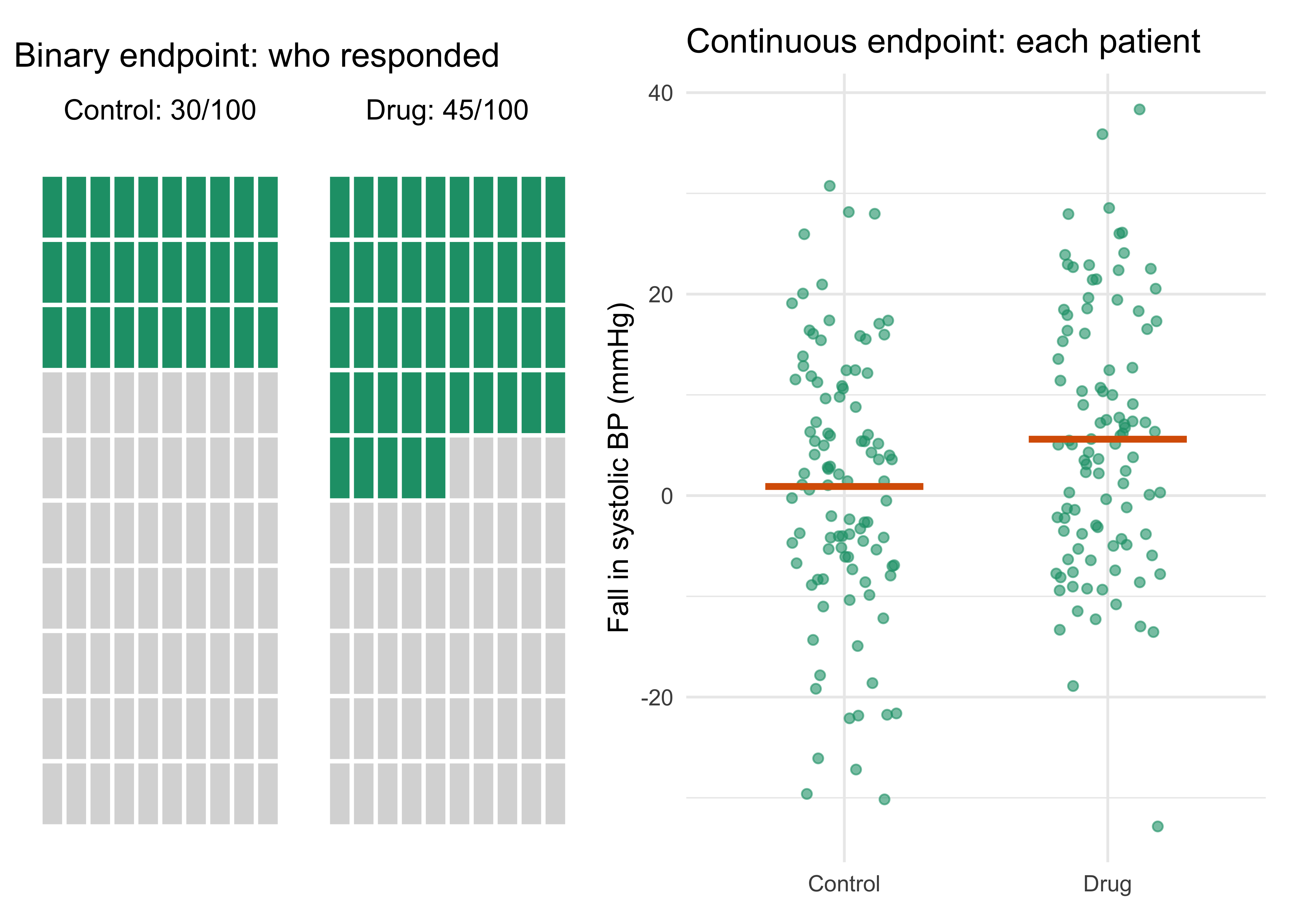
The first thing to see is variation between patients. Figure 4.1 shows one simulated trial of each kind. In the binary version each square is a patient, filled if they responded. Nobody’s response is a fixed property of the drug: among 100 patients on control, about 30 respond, and which 30 is not something we can predict. In the continuous version each dot is a patient’s blood pressure fall. The two clouds overlap heavily. Many patients on the drug do worse than the average patient on control, and many on control do better than the average patient on the drug.
Show the R code
set.seed(2032)y0 <-rep(1:0, c(30, 70)); y1 <-rep(1:0, c(45, 55)) # binary outcomesc0 <-rnorm(100, 0, 12); c1 <-rnorm(100, 4, 12) # BP fall, true means 0 and 4sq <-data.frame(arm =rep(c("Control", "Drug"), each =100), y =factor(c(y0, y1)), i =0:99)sq$x <- sq$i %%10+12* (sq$arm =="Drug"); sq$r <-9- sq$i %/%10pa <-ggplot(sq, aes(x, r, fill = y)) +geom_tile(colour ="white", linewidth =0.8) +scale_fill_manual(values =c("grey85", "#1B9E77"), guide ="none") +theme_void() +annotate("text", x =c(4.5, 16.5), y =10.5, label =c("Control: 30/100", "Drug: 45/100")) +labs(title ="Binary endpoint: who responded")bp <-data.frame(arm =rep(c("Control", "Drug"), each =100), fall =c(c0, c1))pb <-ggplot(bp, aes(arm, fall)) +geom_jitter(width =0.2, height =0, alpha =0.6, colour ="#1B9E77") +stat_summary(fun = mean, geom ="crossbar", width =0.6, colour ="#D95F02") +labs(x =NULL, y ="Fall in systolic BP (mmHg)", title ="Continuous endpoint: each patient")pa + pb
Figure 4.1: One simulated trial with 100 patients per arm. Left: binary endpoint (filled square = responded; 30 of 100 on control, 45 of 100 on drug). Right: continuous endpoint (each dot is one patient’s fall in systolic blood pressure, mmHg; horizontal bar = arm mean). The arms differ on average, but the individual patients overlap heavily.
In this particular trial the binary data show 30 responders on control and 45 on the drug, so the observed difference is exactly the true 15 points. That is a coincidence we arranged on purpose, so that the arithmetic stays clean. The continuous data show means of 0.90 mmHg on control and 5.60 mmHg on the drug, an observed difference of 4.69 against a truth of 4. That is the more typical situation: the data are close to the truth but not equal to it.
This overlap is what D. R. Cox had in mind when he wrote about the comparison of treatments in the presence of what he called large uncontrolled variations between experimental units (Cox 1958). If every patient responded identically to a given treatment, one patient per arm would settle the matter. Because they do not, a single difference in averages comes with a question attached: would we have seen a gap like this anyway, from the luck of which patients landed where? A test is a procedure for answering that question honestly.
A word on what the data cannot tell us. Each patient has, in principle, two potential outcomes, one under each treatment, and we see only one of them. The laboratory module that accompanies this chapter draws the unseen outcomes as faded cells for this reason. Randomization is what lets the observed gap stand in for the unobservable average difference between the two potential outcomes, and Chapter 5 takes that argument up properly. For now it is enough that patients were assigned by a coin, so the two arms are alike apart from chance and the drug.
4.2 The same trial, rerun ten thousand times
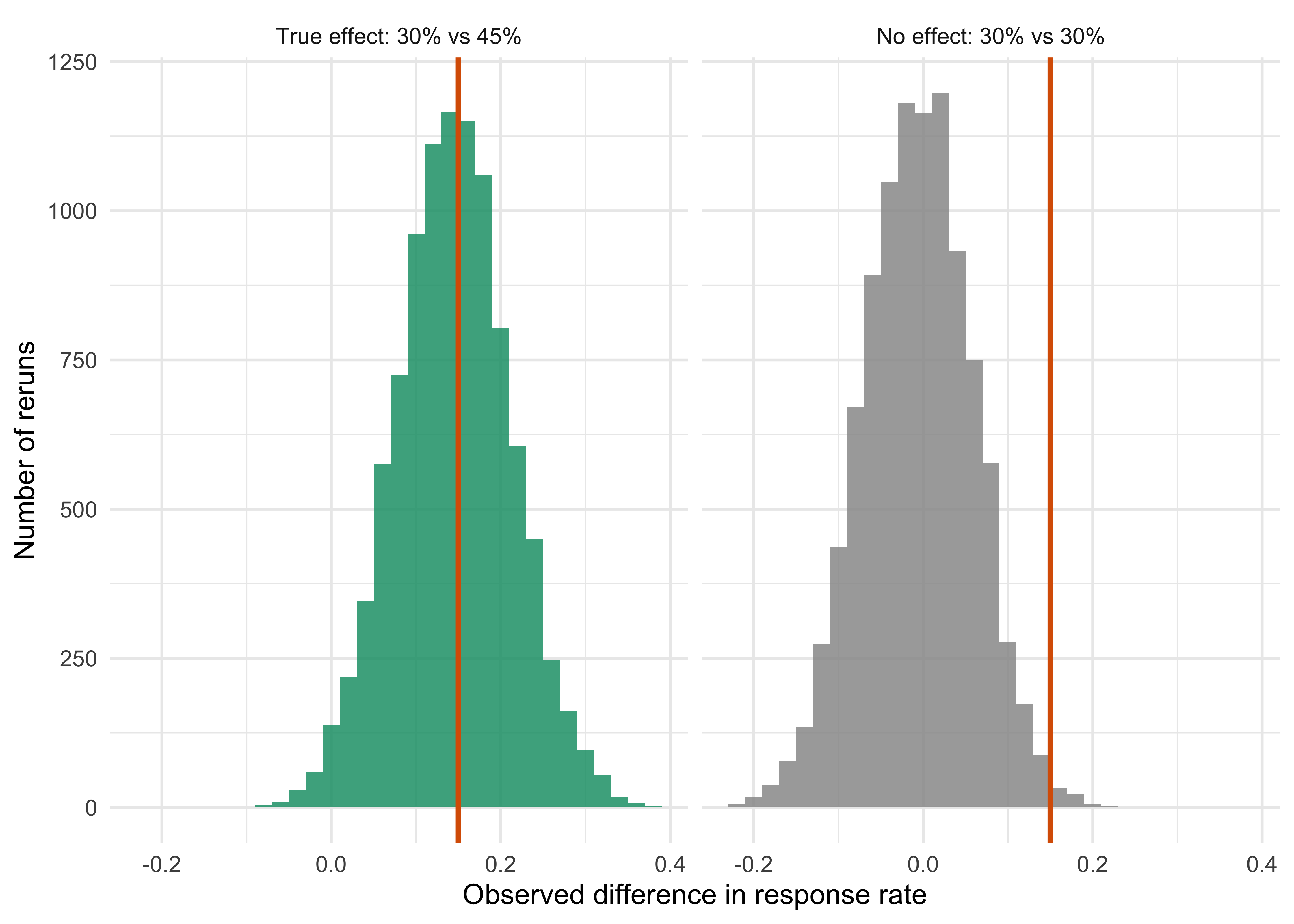
Here is the experiment that makes the rest of the chapter easy. Take the binary trial and rerun it. Draw 100 new control patients with a 30% chance of responding, 100 new drug patients with a 45% chance, and compute the observed difference in response rates. Do it again. Do it ten thousand times. We cannot run a real trial ten thousand times, but a computer can, and the resulting histogram is the sampling distribution of the observed difference: the pattern of results the trial design produces, given a truth.
Show the R code
alt <-sim_two_arm_binary(0.30, 0.45, 100, 10000, seed =11)$diffnul <-sim_two_arm_binary(0.30, 0.30, 100, 10000, seed =12)$diffd <-data.frame(diff =c(alt, nul), world =factor(rep(c("True effect: 30% vs 45%", "No effect: 30% vs 30%"), each =10000), levels =c("True effect: 30% vs 45%", "No effect: 30% vs 30%")))ggplot(d, aes(diff, fill = world)) +geom_histogram(binwidth =0.02, boundary =-0.01, alpha =0.85, show.legend =FALSE) +geom_vline(xintercept =0.15, colour ="#D95F02", linewidth =1) +facet_wrap(~world) +scale_fill_manual(values =c("True effect: 30% vs 45%"="#1B9E77", "No effect: 30% vs 30%"="grey60")) +labs(x ="Observed difference in response rate", y ="Number of reruns")
Figure 4.2: The observed difference in response rates in 10,000 reruns of the same trial (100 per arm). Left: the world where the drug raises the response rate from 30% to 45%. Right: the world where the drug does nothing (both arms 30%). The vertical line is the difference we observed, 0.15.
Three things stand out. First, the histogram on the left is centered on the truth, 0.15, so the observed difference is an unbiased estimate of the effect: right on average, wrong in any single trial. Second, it is spread out. The standard deviation is about 0.067, so a trial that estimates 0.15 could easily have estimated 0.08 or 0.22 and nothing about the drug would have been different. In about 1.7% of reruns, a drug that truly works shows no benefit at all or a harm. Third, the histogram on the right, for a drug that does nothing, is not a spike at zero. It is a hill of about the same width centered on zero, and its upper tail is not empty: in roughly 1.0% of those reruns the observed difference is 0.15 or larger, which is the gap we saw. A drug that does nothing produces a result as good as ours about 1 time in 100. The p-values of the next sections (0.014 to 0.021, depending on the method) are the same idea computed from the data of one trial, and they differ from this 1.0% because a real trial does not know that both arms are at 30%.
That last sentence is, in essence, a p-value, built from the picture and not from a formula. The same logic applied to RECOVERY’s 28-day mortality comparison is in Section 4.11. To turn it into a method we must find a way to learn the right-hand histogram from the data of one trial, because in a real trial we do not know that both arms are 30%. The next two sections give two ways to do this.
The width of the histogram has a formula worth knowing. The standard deviation of the observed difference, called the standard error, is
which for our numbers is \(\sqrt{0.3 \times 0.7/100 + 0.45 \times 0.55/100} = 0.0676\), matching the simulation. For the continuous endpoint, with common standard deviation \(\sigma\), it is \(\sigma\sqrt{2/n} = 12\sqrt{2/100} = 1.70\) mmHg. Two features matter for planning. The standard error shrinks like \(1/\sqrt{n}\), so halving it requires quadrupling the trial. And it grows with the variability of the outcome: noisier patients mean wider histograms, which is why trials work so hard on reducing measurement noise.
4.3 The randomization test: shuffle the labels
The simplest honest test uses nothing but the randomization the trial already performed. Suppose the drug does nothing at all, a claim that Fisher called the null hypothesis (Fisher 1935). Then each patient’s outcome would have been what it was whatever arm they were assigned to (Fisher’s sharp null, which is stronger than a zero average effect, because opposing individual effects can average to zero; Chapter 5 gives the full definition), and the label “drug” or “control” on a patient is just the result of the coin. Under that hypothesis, a different toss of the coins would have produced the same 200 outcomes, dealt into the two arms differently. So we can imitate the coin: pool the 200 outcomes, shuffle the labels, deal 100 into a “drug” arm and 100 into a “control” arm, and compute the difference. Repeat many times. The histogram of those differences shows what chance alone does to this particular set of 200 patients.
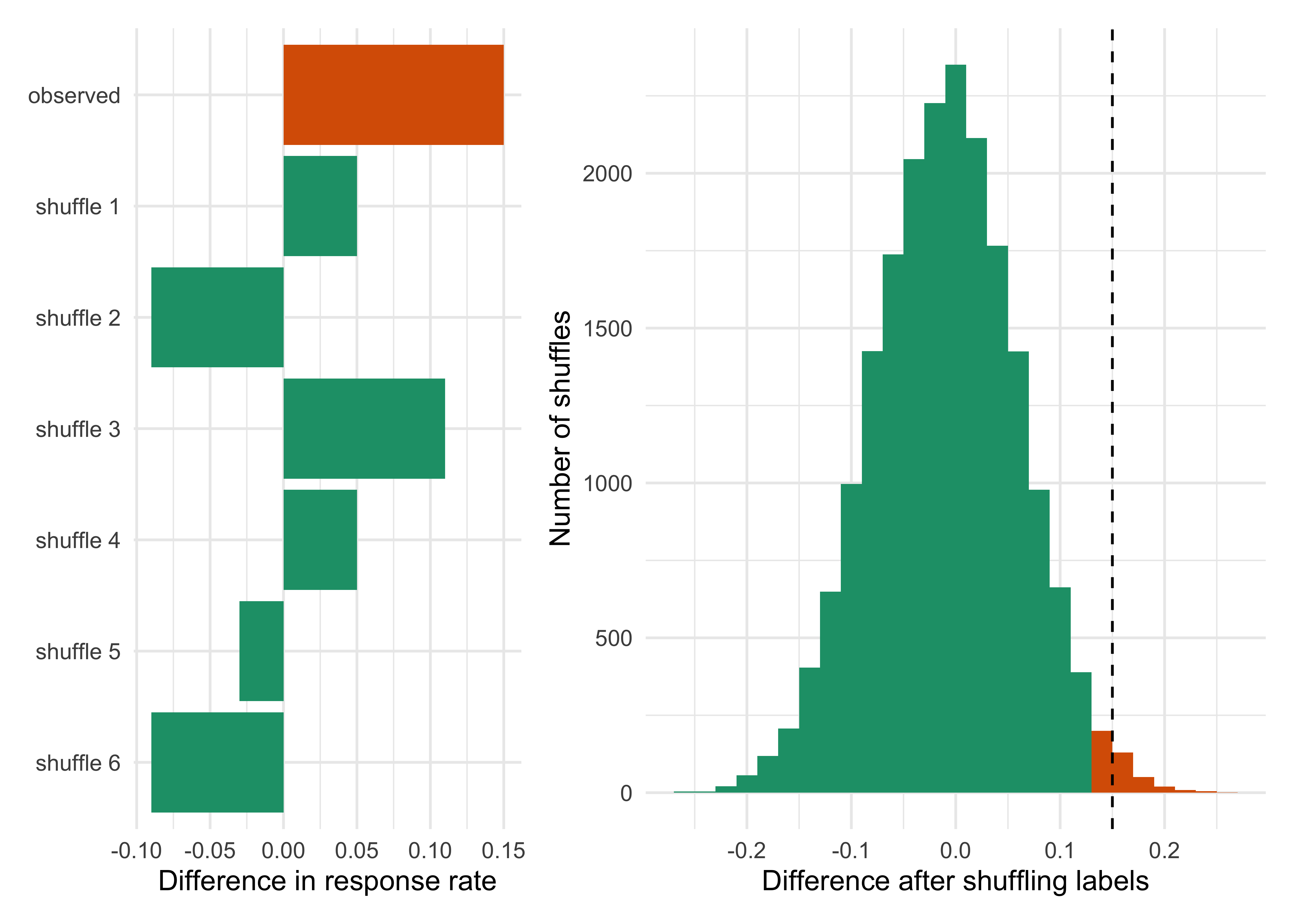
Figure 4.3 first shows the idea on a handful of shuffles, then the histogram from 20,000 of them, with the observed difference marked. The share of shuffles at least as large as the observed difference is the randomization p-value.
Show the R code
pt <-perm_test(y1, y0, nsim =20000, seed =5)six <-perm_test(y1, y0, nsim =6, seed =7)$simsl <-data.frame(who =factor(c("observed", paste("shuffle", 1:6)), levels =rev(c("observed", paste("shuffle", 1:6)))), d =c(pt$obs, six))pl <-ggplot(l, aes(d, who, fill = who =="observed")) +geom_col(show.legend =FALSE) +scale_fill_manual(values =c("#1B9E77", "#D95F02")) +labs(x ="Difference in response rate", y =NULL)s <-data.frame(d = pt$sims, hit = pt$sims >= pt$obs -1e-12)pr <-ggplot(s, aes(d, fill = hit)) +geom_histogram(binwidth =0.02, boundary =-0.01, show.legend =FALSE) +scale_fill_manual(values =c("#1B9E77", "#D95F02")) +geom_vline(xintercept = pt$obs, linetype =2) +labs(x ="Difference after shuffling labels", y ="Number of shuffles")pl + pr +plot_layout(widths =c(1, 1.6))
Figure 4.3: The randomization test for the binary trial. Left: the observed gap (0.15) and six individual re-deals of the same 200 outcomes into two arms of 100. Right: the differences from 20,000 re-deals; the orange area is the share at least as large as the observed 0.15, which is the one-sided randomization p-value.
The one-sided randomization p-value is about 0.021 and the two-sided one about 0.041. In words: if the drug had no effect on any patient, then only about 2.1% of the possible ways the coins could have fallen would give the drug arm 15 or more additional responders. The two-sided version counts gaps of 15 points in either direction, so it roughly doubles.
Notice what this test assumed. It did not assume a bell curve, or a model for how responses arise, or a large sample. It assumed that the labels were assigned by chance and that, if the drug is useless, the outcomes do not depend on the label. The analysis is justified by the randomization in the design, which is exactly the position Fisher took, and which ICH E9 endorses when it calls randomization “a deliberate element of chance” in the assignment (section 2.3.2). The same shuffle works for the continuous endpoint. Pool the 200 blood pressure changes, deal them into two arms of 100, and compute the difference in means. For the continuous trial of Figure 4.1 the observed difference is 4.69 mmHg, and the one-sided randomization p-value is about 0.005 (two-sided about 0.011).
Table 4.1: Randomization test for the continuous endpoint (20,000 shuffles).
Quantity
Value
Observed difference (mmHg)
4.693
One-sided p-value
0.005
Two-sided p-value
0.011
SD of shuffled differences (mmHg)
1.850
Planning formula, sigma*sqrt(2/n) (mmHg)
1.697
Table 4.1 gives the result. The shuffled differences have a standard deviation of 1.85 mmHg. That is a little above the 1.70 of the formula because this sample’s standard deviations (13.0 and 12.9) exceed the planning value of 12; it is close to the data-based standard error of 1.83. This anticipates the next section: the shuffling distribution is a bell curve with a width we can write down.
Two practical remarks. A shuffle test is a clean way to check any other test, because it makes so few assumptions. And in the binary case the shuffling can be done exactly, by counting, instead of by simulation. The exact count is Fisher’s exact test, whose two-sided p-value here is 0.0405, which matches our simulation. In real trials, with stratified randomization or a covariate-adjusted analysis, the shuffle must respect the randomization scheme, so only labels within a stratum are exchanged. That connection between the design and the analysis is the subject of Chapter 5.
4.4 The normal approximation and the z test
Shuffling is correct but heavy, and it was laborious before computers (exact enumeration and manual randomization tests existed long before them, but they were practical only for very small trials). The histograms we have drawn all look like bell curves. This is not an accident: the observed difference is an average of many small independent contributions, one from each patient, and the central limit theorem says that such sums settle into a normal distribution as \(n\) grows. This lets us replace the shuffling with a formula.
Under the null hypothesis, where the drug does nothing, the difference in response rates is approximately normal with mean zero and standard error computed from the pooled response rate \(\bar p = (x_0 + x_1)/(2n)\), where \(x_j\) is the number of responders in arm \(j\):
The pooling uses the null hypothesis that both arms have the same \(p\). For the continuous endpoint the statistic is the difference in means divided by \(\sqrt{s_1^2/n + s_0^2/n}\), with \(s_j\) the sample standard deviation in arm \(j\). We then ask how far out in the tail of a standard normal curve \(Z\) falls. A value of \(Z\) means “this many standard errors from zero”, and the book’s notation \(z_\alpha\) is the upper \(\alpha\) quantile of the standard normal, so \(z_{0.025} = 1.96\).
For the binary trial, \(\bar p = 0.375\), the standard error is 0.0685, and \(Z = 0.15/0.0685 = 2.19\). The upper normal tail beyond 2.19 is 0.0142, so the one-sided p-value is 0.014 and the two-sided one is 0.029. For the continuous trial, \(Z = 4.69/1.83 = 2.56\), with one-sided p-value 0.0052.
Show the R code
pb <- (30+45) /200; seb <-sqrt(2* pb * (1- pb) /100); sec <-sqrt(var(c1) /100+var(c0) /100)pn <-function(s, se, xl) ggplot(data.frame(d = s), aes(d)) +geom_histogram(aes(y =after_stat(density)), bins =50, fill ="#1B9E77", alpha =0.5) +stat_function(fun = dnorm, args =list(sd = se)) +labs(x = xl, y =NULL) +theme(axis.text.y =element_blank())pn(pt$sims, seb, "Difference in response rate") +pn(pc$sims, sec, "Difference in mean BP fall (mmHg)")zb <-z_test_binary(30, 45, 100); zc <- (mean(c1) -mean(c0)) / sec
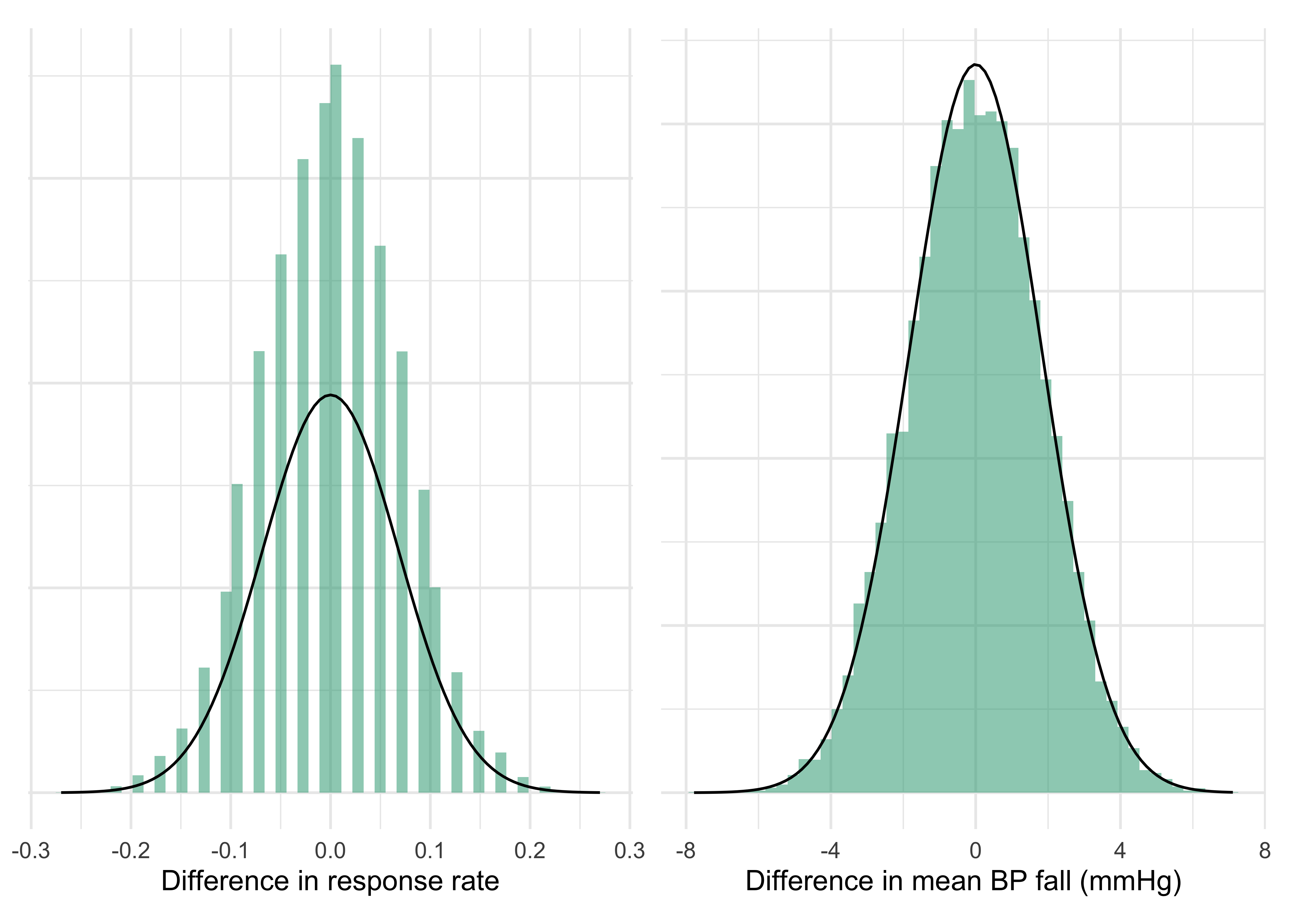
Figure 4.4: The shuffling distributions of the two endpoints (histograms) against the normal curve the z test uses (line). The curve is almost on top of the histogram for the continuous endpoint. For the binary endpoint the histogram moves in steps, because the response counts are whole numbers.
Table 4.2 puts the three methods side by side. The randomization test and the z test agree closely for the continuous endpoint. For the binary endpoint they disagree more than a reader might expect: one-sided 0.021 by shuffling against 0.014 by the normal curve. The reason is visible in the left panel of Figure 4.4. The shuffled differences can only take values in steps of 2/100 on a difference scale, and the “at least 0.15” tail includes the whole step at 0.15, while the normal curve effectively counts only half of that step. The standard remedy is a continuity correction, which moves the cutoff half a step, from 0.15 to 0.14 (which gives \(Z = 2.04\) and a one-sided p-value near 0.021). The lesson for a protocol is that the normal approximation is an approximation, and with a binary endpoint, moderate \(n\) and a p-value close to the threshold, the choice of test statistic can change the verdict. This is why statistical analysis plans name the test exactly (Pearson chi-square, Fisher exact, with or without continuity correction) before any data exist.
Table 4.2: The same trial analyzed by several methods. Shuffle values carry Monte Carlo error of about 0.001.
Endpoint
Method
One-sided p
Two-sided p
Binary (30 vs 45 of 100)
Randomization (shuffle)
0.021
0.041
Binary
Fisher exact
0.020
0.041
Binary
z test, pooled (no correction)
0.014
0.028
Continuous (mean difference 4.69)
Randomization (shuffle)
0.005
0.011
Continuous
z test
0.005
0.010
Continuous
t test
0.006
0.011
NoteTechnical note: why \(Z\) is approximately standard normal
Write the difference in means as \(\bar Y_1 - \bar Y_0\). Each mean is an average of \(n\) independent terms, so by the central limit theorem it is approximately normal with mean \(\mu_j\) and variance \(\sigma_j^2/n\). The difference of independent normals is normal with variance \(\sigma_1^2/n + \sigma_0^2/n\). Dividing by the standard error gives a statistic that is approximately \(N(0,1)\) under the null. For the binary endpoint the variance of a single response is \(p(1-p)\), which is what Equation 4.1 uses. When the variance is estimated from the data and \(n\) is small, the reference distribution is a Student \(t\) with slightly heavier tails, but with 100 patients per arm the difference is in the third decimal (the 97.5th percentile is 1.972 on 198 degrees of freedom against 1.960).
For the clinician: the approximation fails when responses are rare, when \(n\) is small, or when the outcome has extreme values that dominate the mean. In those situations use the exact or shuffle versions, and make the choice in the protocol.
4.5 The p-value, defined carefully
Both tests produced a number called the p-value. It is worth defining it once with care, because everything about misuse starts with sloppy definitions. The ingredients are three: a null hypothesis, a test statistic, and the data.
The null hypothesis\(H_0\) is the claim that the treatment effect is zero, \(\theta = 0\) (or, for a one-sided test, \(\theta \le 0\)), a statement about the average effect and weaker than the sharp null of the randomization test. The test statistic is a summary of the data that is large when the data favor the drug: here, the observed difference or the \(Z\) derived from it. The p-value is then
\[
p \;=\; \mathbb{P}\bigl(\text{test statistic at least as favorable to the drug as the one observed} \;\bigm|\; H_0 \text{ true}\bigr) ,
\tag{4.3}\]
where the probability is over the repetition of the trial, in the sampling sense of the previous sections. That is the share of the right-hand histogram of Figure 4.2 beyond the observed value. It is the answer to the question “if nothing is going on, how often would luck look this good?”
The definition has several consequences that are easy to forget.
The probability is about the data, given the hypothesis. It is not the probability of the hypothesis given the data. A p-value of 0.014 does not mean a 1.4% chance that the drug does not work, and its complement is not the probability that the drug works. Getting from data to the probability of a hypothesis needs a prior, which is the subject of Chapter 6.
It depends on the plan, not only on the data. The same sequence of 9 heads and 3 tails has different p-values if the experimenter planned 12 flips or planned to stop at the third tail, because “as extreme or more” is evaluated over the trials one could have run. In trial language, a p-value depends on the stopping rule and on the number of analyses. This is the reason interim looks must be pre-specified, and it is the starting point of Chapter 11.
It depends on how many questions were asked. A p-value of 0.03 for the one endpoint the protocol named in advance and a p-value of 0.03 for the best of twenty endpoints are not the same evidence. ICH E9 section 5.6 states that multiplicity “may necessitate an adjustment to the type I error”, and Chapter 10 treats the methods.
It mixes the size of the effect with the size of the trial. A tiny and clinically irrelevant difference gives a tiny p-value in a huge trial, and a large and important difference can give an unimpressive p-value in a small one. The p-value says nothing about whether the effect is worth having. That is the job of the estimate and its interval.
A large p-value is not evidence of no effect. It says the data were not surprising under the null. They may be even less surprising under a real and useful effect, and in a trial of 50 per arm the 30% versus 45% drug has a power near one in three (the next sections explain what that means).
The American Statistical Association’s statement on p-values collects these points (Wasserstein and Lazar 2016), and Goodman’s “dirty dozen” lists twelve misreadings that survive in the clinical literature (Goodman 2008). We return to the evidential meaning of a p-value, and to what a Bayes factor or a posterior probability would say about the same data, in Chapter 7.
To turn a p-value into a decision, we need a threshold. The protocol fixes a level \(\alpha\) in advance, and rejects \(H_0\) if \(p \le \alpha\). That is a decision rule with a known long-run error rate, and the next sections look at what the rule does when the drug works and when it does not.
4.6 Confidence intervals
A p-value says whether the data are compatible with no effect. It does not say what effect is likely, and a decision about a drug needs both. A confidence interval reports the range of effect sizes that the data do not rule out. For a difference with an approximately normal estimator the 95% interval is the estimate plus and minus 1.96 standard errors:
For the binary trial the standard error with unpooled rates (Equation 4.1, estimated) is 0.0676, so the 95% interval for the risk difference is \(0.15 \pm 0.132\), that is, 0.017 to 0.283. The data are compatible with a gain as small as 2 percentage points and as large as 28. For the continuous trial the interval is \(4.69 \pm 1.96 \times 1.83\), that is, 1.10 to 8.28 mmHg. Neither interval contains zero, which agrees with the two-sided tests that gave p-values below 0.05.
The interval is wide, and this is not a flaw of the method. It tells the truth about a trial of 100 per arm: a response-rate gain of 2 points and one of 28 points are both consistent with what we saw, and they would lead to different decisions about whether the drug is worth developing. ICH E9 section 5.5 asks that estimates of treatment effects “should be accompanied by confidence intervals, whenever possible”. The reason is that a bare p-value hides this width.
What the 95% refers to
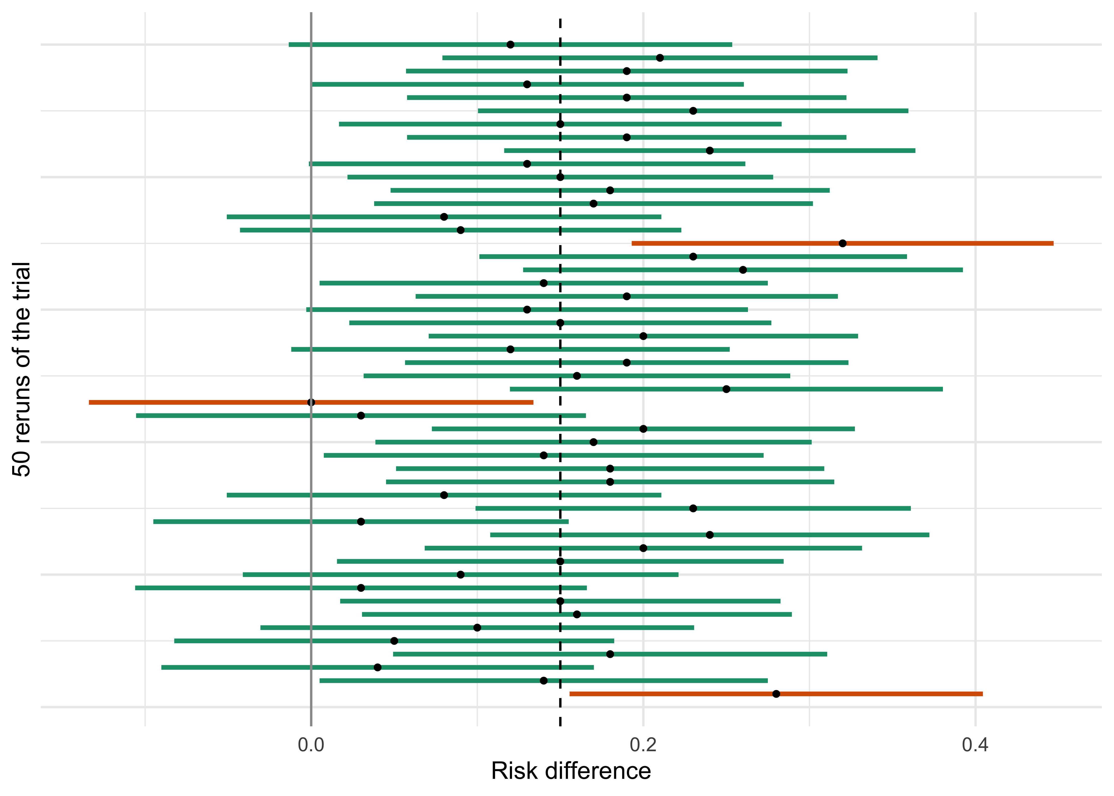
The correct reading of “95%” is about the procedure, not about one interval. If the same trial were rerun many times and an interval computed each time, about 95% of the intervals would contain the true effect. Figure 4.5 shows 50 reruns of the binary trial, with the true difference of 0.15 marked.
Figure 4.5: Fifty reruns of the binary trial, each with its own 95% Wald interval for the risk difference. The vertical line is the truth (0.15). Orange intervals miss it. In the long run about 5% of intervals miss; in 50 trials the count is itself random.
Over 100,000 reruns the Wald interval covers the truth in 94.8% of reruns, close to the nominal 95%. That shortfall is a property of the normal approximation again, as with the p-values; better-behaved intervals for proportions exist, for example the score-based interval that Newcombe compared with ten other methods (Newcombe 1998). The practical rule is the one for tests: name the interval method in the analysis plan.
Notice also what the interval is not. It is not a statement that there is a 95% chance that the true difference lies in 0.017 to 0.283. Once computed, the interval either contains the truth or does not, and the 95% describes the method’s long-run record. A statement of the form “given these data, the probability that the effect lies in this range is 95%” is a different object, a credible interval, and requires a prior. For a large trial with little prior information the two usually agree numerically, which is why the common misreading rarely does damage, but the distinction matters when the sample is small, the prior is informative, or when we want to evaluate a decision rule. Chapter 6 returns to it.
Tests and intervals are the same thing
A confidence interval and a test are two views of one calculation. The 95% two-sided interval contains exactly the values \(\theta_0\) that a two-sided test at the 5% level would not reject: if you ask “can we reject that the true difference is \(\theta_0\)?” for every \(\theta_0\), the ones you cannot reject form the interval. This is the duality. It has a protocol consequence. A test of no effect asks only whether 0 is in the interval, but the same machinery also lets you test other hypotheses, such as “the benefit is at least 5 points”, by checking whether the relevant confidence bound (here the lower limit of a one-sided interval) is above 5, not merely whether 5 lies inside a two-sided interval. Non-inferiority testing rests on this: the null hypothesis is that the new treatment is worse than control by at least the margin, and the test is whether the lower end of a one-sided interval clears the margin.
It also explains why ICH E9 links the two. The same section that calls for confidence intervals, section 5.5, says the one-sided type I error should be set at half of the two-sided one, and gives the reason: “This promotes consistency with the two-sided confidence intervals that are generally appropriate for estimating the possible size of the difference between two treatments.” A one-sided test at 0.025 rejects essentially when the lower limit of the two-sided 95% interval is above zero, so the result in the CSR (a p-value) and the figure in the abstract (an interval) cannot disagree in any material way. (The equivalence is exact only when the test and the interval use the same standard error. Our binary trial uses 0.0685 in the pooled test and 0.0676 in the interval, so a result very close to the line could fall on different sides.)
For the binary trial, the lower limit of the interval is 0.017, above zero, and the one-sided p-value from the normal test (0.014) is below 0.025. For the continuous trial the lower limit is 1.10 and the one-sided p-value is 0.005. Both trials “succeed” on the regulatory convention, though the binary one only just, and the width of its interval is a more honest summary than the verdict.
4.7 Two kinds of error, and power
So far we have asked what the data say about one trial. A regulator, a sponsor and a patient also want to know how often the decision rule, “reject \(H_0\) if \(p \le \alpha\)”, gives the wrong answer. There are two ways to be wrong, and they are not symmetric. The language of type I and type II errors and of power is Neyman and Pearson’s (Neyman and Pearson 1933). Fisher’s p-value as a measure of evidence against a null hypothesis, and the 0.05 convention, come from his work (Fisher 1935, 1946).
A type I error is rejecting \(H_0\) when the drug has no effect: approving something useless. A type II error is failing to reject \(H_0\) when the drug does work: abandoning something useful. The probability of a type I error is the level of the test, \(\alpha\). The probability of a type II error is \(\beta\), and the probability of avoiding it, \(1 - \beta\), is the power. Notice that \(\alpha\) is a probability computed under the null world and that \(\beta\) is computed under a specific alternative. Power is not a single number for a trial but a function of the true effect, and when someone quotes “90% power” the first question is: for what effect?
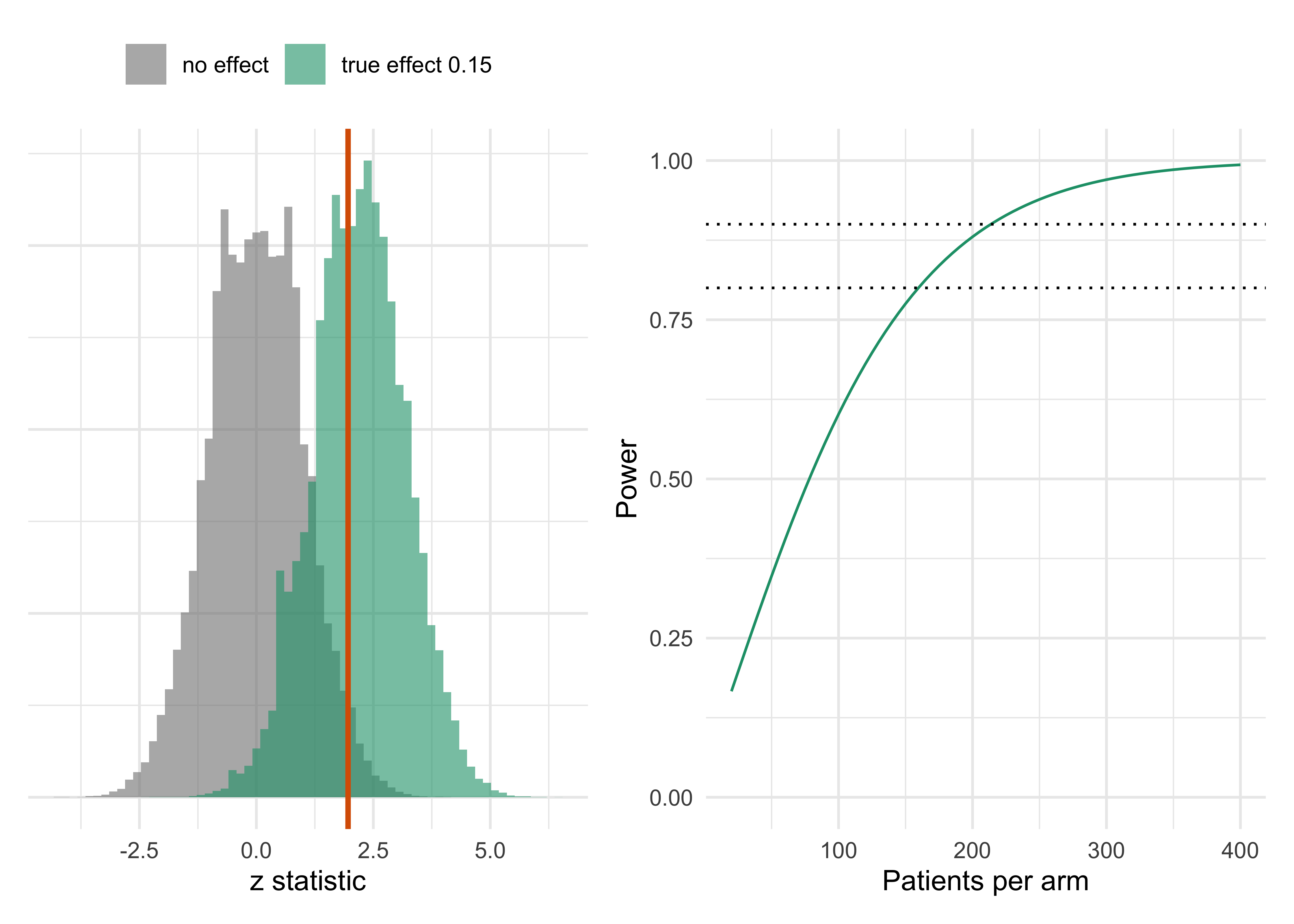
We can read both off the simulation of Figure 4.2. Run the same trial many times, apply the decision rule each time, and count rejections. In the world where the drug does nothing the rejection rate is the type I error rate, and it is close to the nominal 2.5% when we reject for \(Z > 1.96\). In the world with the true 15-point effect the rejection rate is the power.
Show the R code
n0 <-sim_two_arm_binary(0.30, 0.30, 100, 100000, seed =31); n1 <-sim_two_arm_binary(0.30, 0.45, 100, 100000, seed =32)zn <-z_test_binary(n0$x0, n0$x1, 100); za <-z_test_binary(n1$x0, n1$x1, 100)pw <-function(n) pnorm(1.96-0.15/sqrt(0.3*0.7/ n +0.45*0.55/ n), lower.tail =FALSE)z <-data.frame(z =c(zn, za), world =rep(c("no effect", "true effect 0.15"), each =100000))p1 <-ggplot(z, aes(z, fill = world)) +geom_histogram(binwidth =0.17, position ="identity", alpha =0.6) +geom_vline(xintercept =1.96, colour ="#D95F02", linewidth =1) +scale_fill_manual(values =c("grey50", "#1B9E77")) +labs(x ="z statistic", y =NULL, fill =NULL) +theme(axis.text.y =element_blank(), legend.position ="top")p2 <-ggplot(data.frame(n =seq(20, 400, 5)), aes(n, pw(n))) +geom_line(colour ="#1B9E77") +geom_hline(yintercept =c(0.8, 0.9), linetype =3) +ylim(0, 1) +labs(x ="Patients per arm", y ="Power")p1 + p2
Figure 4.6: Left: the z statistic in 100,000 reruns with no effect (grey) and with the true 15-point effect (teal), 100 patients per arm. Reruns to the right of 1.96 reject the null. The grey area beyond 1.96 is the type I error (2.5%); the teal area beyond 1.96 is the power (60%); the teal area to its left is the type II error. Right: power of the one-sided 0.025 test against the number of patients per arm.
The type I error is held at about 2.5%, because that is what the threshold 1.96 was chosen to do. The power at 100 patients per arm is 60%: if the drug truly lifts the response rate from 30% to 45%, this trial would detect it about six times in ten. The other four times, a drug that works would be missed. Our observed trial, with \(Z = 2.19\), happens to be one of the six. It would be wrong to read that as evidence that the trial was well designed. The right-hand panel shows that power rises with the number of patients: roughly 35% at 50 per arm, 60% at 100, 78% at 150, 88% at 200, 94% at 250 and 97% at 300. The customary targets of 80% or 90% need roughly 160 to 215 patients per arm for this effect. The continuous trial, with a 4 mmHg effect and standard deviation of 12 mmHg, has power of about 65% at 100 per arm.
The two errors trade against each other. Lower \(\alpha\) to reduce false positives and the rejection region shrinks, so power falls. Raise \(\alpha\) and power rises, along with the chance of approving something useless. The only way to improve both at once is to make the standard error smaller, with more patients, a less noisy endpoint, or better use of information, and this is where the later chapters of the book make their case. The size of a trial is dictated by the question “how many patients make both errors acceptably small?” and the answer is a formula in \(\alpha\), \(\beta\), the effect and the variance that Chapter 9 develops. A guide for the reader who wants the shape now: for a one-sided \(\alpha = 0.025\) and 90% power, the number of patients needed is proportional to \((z_{0.025} + z_{0.10})^2 = 10.51\) divided by the squared standardized effect.
It is worth stating who bears each error. A type I error falls mostly on future patients, who receive a drug that does not work, and on the regulator who approved it. A type II error falls on future patients too, who will not receive a drug that would have helped, and on the sponsor who abandoned it. Regulators fix \(\alpha\) by convention and leave \(\beta\) to the sponsor’s judgment, which is why the traditional design is organized around the type I error and why sponsors, who pay for the type II error, ask for more efficient designs. Module 03 of the laboratory, errors and power (https://nytel.ai/testing/03-errors-power.html), lets you move the slider and see the two areas trade off.
4.8 One-sided or two-sided, and why 0.025
We have used both kinds of p-value, so we must say which one counts. A two-sided test counts departures from the null in either direction as evidence: the drug might help or harm, and the test is alert to both. A one-sided test counts only departures in the direction of benefit. In the shuffle picture the one-sided p-value is the orange tail on the right, and the two-sided is that tail plus its mirror image on the left (twice as large, when the reference distribution is symmetric).
The argument for the two-sided test is that a trial should be able to detect harm, and that a one-sided test with a generous level appears to lower the bar. The argument for the one-sided test is that the regulatory question for a new drug is asymmetric: approval depends on benefit being demonstrated, and a harmful drug is, for the purpose of the efficacy decision, not approved either way. Harm shows up in the safety analyses and in the interim monitoring by the data monitoring committee.
The regulatory convention resolves the matter in a way that keeps both arguments. ICH E9 section 5.5 asks the sponsor to say in the protocol whether one- or two-sided tests will be used and to “justify prospectively the use of one-sided tests”. It then states the rule that decides the practical question: “The approach of setting type I errors for one-sided tests at half the conventional type I error used in two-sided tests is preferable in regulatory settings.” With the conventional two-sided level of 0.05, half is 0.025. That is the origin of the book’s default: a one-sided level of \(\alpha = 0.025\) is the same evidential bar as a two-sided level of 0.05, as the confidence interval duality of the previous section shows: both reject when the 95% interval excludes zero on the favorable side. The more recent FDA draft guidance on Bayesian methodology uses exactly this language, describing the usual standard as performing a statistical hypothesis test at a one-sided significance level of 0.025 (section IV.A, draft, January 2026, non-binding) (U.S. Food and Drug Administration 2026).
Two practical consequences follow. First, when a paper reports “p = 0.04, two-sided” for a drug that helped, the one-sided equivalent is 0.02, and the trial meets the 0.025 bar. When a paper reports “one-sided p = 0.04”, it does not, and the usual regulatory reading would be that the trial missed. Always check which p-value is quoted. Our binary trial is a live example of this edge: the normal z test gives a one-sided p-value of 0.014, the Fisher exact test 0.020 and the randomization test 0.021. All three clear 0.025, but the last two with little room. The claim “the drug works” is the same in each, but the margin is slim. Second, the sample size formula contains \(z_{0.025} = 1.96\) for one-sided designs, which is the same number as the two-sided 5% critical value, so the trial size is the same under either label provided the conventions are matched.
It is also possible to be tempted by the one-sided test in the wrong way. If the sponsor looks at the data, sees the drug is ahead, and then declares a one-sided test at 0.05, the type I error rate has doubled to 5% for a drug that does nothing, and the test is no longer prospectively justified. This is why E9 says what it says, and why the statistical analysis plan fixes the side, the level and the test before unblinding. The trap in the other direction is that a one-sided 0.025 test gives no formal weight to results in the harmful direction. A trial can end with a strongly negative difference and a one-sided p-value near 1, which is true but uninformative; the safety review and monitoring plan, and not the efficacy test, are where harm is handled.
4.9 Noninferiority and equivalence: testing against a margin
Every test so far asked whether the drug beats a comparator. Many trials ask a different question. When an effective treatment already exists, withholding it in favor of placebo is often unethical, so the new drug is compared with the active control, and the claim is that it is not unacceptably worse, perhaps because it is safer, cheaper, easier to take, or because the trial is an outcomes trial in which the new drug is expected to help the heart as well as lower glucose. This is a noninferiority trial, and its logic is the logic of this chapter with the null hypothesis moved.
Let \(\gamma = \log \mathrm{HR}\) be the raw log hazard ratio of the new drug against the active control, a separate symbol from the effect \(\theta\) of the book’s notation because here values above zero mean the new drug is worse. The superiority hypotheses are \(H_0:\gamma\ge 0\) against \(H_1:\gamma<0\). For noninferiority with margin \(M>1\) on the hazard ratio scale, the hypotheses are \[
H_0:\ \gamma \ge \log M \qquad\text{against}\qquad H_1:\ \gamma < \log M.
\tag{4.5}\] Rejecting \(H_0\) means the new drug is shown to be no worse than the margin allows. The test is one-sided at 0.025, exactly as in Section 4.8, and it is equivalent to checking whether the upper limit of the two-sided 95% interval lies below \(\log M\) (Section 4.6). Nothing about the machinery is new; what is new is that the answer depends entirely on \(M\), a number the data do not supply. Putting the burden of proof on the claim of similarity, by reversing the roles of null and alternative, goes back to Dunnett and Gent for equivalence (Dunnett and Gent 1977) and to Blackwelder for noninferiority (Blackwelder 1982).
Where the margin comes from
The FDA guidance on noninferiority trials (final, November 2016) (U.S. Food and Drug Administration 2016) and ICH E10 (International Council for Harmonisation 2000) give the reasoning. A noninferiority trial with no placebo arm cannot show by itself that the new drug works: if the new drug is “not much worse” than a control, and the control was never shown to work in this trial, the comparison is informative only if the control’s effect is known from earlier placebo-controlled trials and is assumed to hold now. The guidance builds the margin in two steps. The first, usually written \(M_1\), is the whole effect of the active control over placebo that the sponsor can reasonably assume in the present trial, estimated from the historical trials (conventionally the conservative limit of a meta-analytic confidence interval, not the point estimate). The second, \(M_2\), is the margin actually used, chosen to preserve a clinically meaningful fraction of that effect, so that \(M_2\le M_1\). How much to preserve is a clinical judgment, and the guidance says the margin should be justified for the setting, not read from a convention. Two ways of using the historical estimate are described (Rothmann and colleagues set out both for noninferiority mortality trials in oncology (Rothmann et al. 2003)): the fixed-margin approach, which sets the margin from the historical confidence limit and then runs an ordinary test, and the synthesis approach, which combines the historical and current estimates directly and carries the uncertainty of both into one test (the Bayesian version is in Section 19.11).
The scheme rests on the constancy assumption: the effect of the active control against placebo, estimated years ago, is the effect it would have had in this trial’s population, with this background care and this endpoint definition. The assumption cannot be checked within the trial, which is why the guidance and ICH E10 attach so much weight to assay sensitivity, the ability of the trial to distinguish an effective treatment from an ineffective one. A noninferiority trial that is sloppy (poor adherence, crossover, loosely defined events) pulls the two arms together and makes any new drug look noninferior, so the usual protections against bias in a superiority trial work in the opposite direction here. Sloppiness helps the sponsor, which is the reason the analysis population also matters. The guidance stresses trial quality and conduct; it does not prescribe a rule that intention-to-treat and per-protocol analyses must agree, though reporting both and examining any discrepancy is common practice.
The margin must be fixed in the protocol and justified before unblinding. A margin that is changed after the data are seen is not a margin.
Equivalence
An equivalence trial asks for the difference to lie inside a two-sided margin, \(-\log M<\gamma<\log M\) on the log scale (the hazard ratio between \(1/M\) and \(M\)). The standard analysis is two one-sided tests (TOST), each at the one-sided level, one against each end of the margin, and equivalence is declared only if both reject; this is the same as the confidence interval lying entirely inside \((-\log M, \log M)\). Bioequivalence studies and some biosimilar comparisons use this form. Most clinical efficacy trials that say “equivalence” mean noninferiority, and the one-sided test is the more common. The upper bound of a two-sided 95% interval is the standard one-sided 0.025 noninferiority test, and noninferiority imposes no corresponding lower-bound requirement. A sponsor who wants noninferiority should say so, and should not frame the trial as equivalence, which adds a lower-bound requirement that the question does not need.
SURPASS-CVOT: a noninferiority margin in practice
SURPASS-CVOT randomized adults with type 2 diabetes and established atherosclerotic cardiovascular disease to tirzepatide or dulaglutide 1.5 mg, with a primary composite of cardiovascular death, myocardial infarction and stroke (Nicholls et al. 2025). Dulaglutide was chosen as the control because REWIND had shown that it reduces cardiovascular events against placebo (Gerstein et al. 2019), which is what makes it a legitimate active comparator. The pre-specified noninferiority margin was 1.05 for the upper limit of the 95.3% confidence interval of the hazard ratio, and superiority would be claimed only if the upper limit were below 1.00. The trial randomized 13,299 patients; the modified intention-to-treat population was 13,165 (6586 on tirzepatide, 6579 on dulaglutide). The primary outcome occurred in 801 patients (12.2%) on tirzepatide and 862 (13.1%) on dulaglutide, with a hazard ratio of 0.92 (95.3% CI 0.83 to 1.01).
Show the R code
hr <-0.92; lo <-0.83; hi <-1.01; M <-1.05zc <-qnorm(1- (1-0.953) /2)se <- (log(hi) -log(lo)) / (2* zc)z_ni <- (log(hr) -log(M)) / sez_sup <-log(hr) / setb <-data.frame(Hypothesis =c("Noninferiority: H0 is HR at least 1.05", "Superiority: H0 is HR at least 1.00"),`z statistic`=round(c(z_ni, z_sup), 2),`One-sided p`=signif(pnorm(c(z_ni, z_sup)), 2),`Upper limit below the bound?`=c("Yes (1.01 < 1.05)", "No (1.01 > 1.00)"),check.names =FALSE)knitr::kable(tb, align ="lrrl")
Table 4.3: SURPASS-CVOT primary outcome, tested against the noninferiority margin 1.05 and against superiority, from the published hazard ratio and its 95.3% interval (normal approximation on the log scale).
Hypothesis
z statistic
One-sided p
Upper limit below the bound?
Noninferiority: H0 is HR at least 1.05
-2.68
0.0037
Yes (1.01 < 1.05)
Superiority: H0 is HR at least 1.00
-1.69
0.0460
No (1.01 > 1.00)
The standard error implied by the published interval is 0.049 on the log scale. Against the margin the one-sided p-value is 0.0037, in line with the reported 0.003 (the reported value comes from the trial’s own analysis, which can differ a little from a calculation on the rounded interval), so noninferiority is established. Against zero the one-sided p-value is 0.05, in line with the reported two-sided 0.09 for superiority, so superiority is not. Both statements come from the same interval. The two tests have two different nulls, and the trial can win the first and lose the second without contradiction. Notice also that the margin did the work: the upper limit 1.01 is above 1.00 and below 1.05, and a margin of 1.00 would have been a superiority trial.
The traditional report stops here: noninferiority met, superiority not met. What it does not give is the probability that the hazard ratio lies below 1.05, below 1.00, or below 0.90, nor the effect against placebo that the dulaglutide comparison implies. The probability that the hazard ratio lies below a given value is a posterior probability, which is where the Bayesian distinction lies. The effect against placebo has frequentist treatments as well, such as the synthesis approach above. Both are taken up in Section 19.11 and Section 19.12.
4.10 Where the traditional trial stands, and what changes next
Put the pieces together and you have the traditional single-look trial. The protocol states the endpoint, the effect to be detected, the one-sided level of 0.025 and the power. It fixes \(n\) from these. The trial runs to completion. The analysis computes a test statistic and a p-value from the pre-specified method, and an interval for the effect. The decision is “success” if the p-value is at most 0.025, one-sided, and the CSR reports the interval alongside. The method is transparent, its error rates are known by construction (type I by the choice of the level, power by calculation or simulation), and it has a regulatory history of decades. It is the benchmark against which every design later in the book is judged. When there is one look, a single primary endpoint and no useful prior information, it is also hard to improve on, and the book says so where it matters (Chapter 21).
What this design does not do is answer the questions a decision maker actually has. The p-value does not give the probability that the drug works, the interval’s 95% is a statement about the procedure, and the error rates describe a procedure that is run once at a fixed sample size, so they change when the trial is monitored, when several endpoints or arms are examined, or when earlier information is brought in. Each of these is a place where the traditional answer needs repair, and where a Bayesian formulation offers another route at a price that the book will itemize. The table summarizes what this chapter established and where the book goes next.
Question
Traditional answer (this chapter)
Where it goes next
Is there a difference?
p-value against \(H_0\): the share of reruns or shuffles at least this extreme
Evidence beyond p-values and Bayes factors (Chapter 7)
Where do the two approaches agree numerically? In a simple setting with a flat prior, the Bayesian posterior probability that the drug is better than control is close to one minus the one-sided p-value. For our continuous trial this is a statement about 0.995, and for the binary trial about 0.986. The agreement is not a coincidence, and it tells us that the Bayesian bar and the traditional bar coincide when there is a single look and no prior information. They diverge once the design is made more flexible, and the point of the book is to show how and by how much.
TipIn the protocol
A statistical section that follows this chapter would state: the primary endpoint (response at week 12, or change from baseline in systolic blood pressure); the null and alternative hypotheses (\(H_0: \theta \le 0\) against \(H_1: \theta > 0\)); the test and its exact form (for the binary endpoint, the pooled z test or Fisher exact test and whether a continuity correction is used; for the continuous endpoint, the t test or an analysis of covariance); the one-sided significance level of 0.025; the effect against which power is calculated and the power; the two-sided 95% confidence interval and its method; the rule on how the randomization scheme enters the analysis; and the statement that none of these will change after unblinding.
TipTry it in the lab
Module 00 at https://nytel.ai/testing/00-are-they-different.html lets you decide “same or different” for rows of 0s and 1s before it reveals the truth, then re-randomize the same data 1,000 times to see how often chance alone makes a gap that large. Predict the p-value from the picture first, then compare with the box; the “Why the coin?” section at https://nytel.ai/testing/00-are-they-different.html#why-coin shows what the shuffling is protecting against. In module 02 at https://nytel.ai/testing/02-p-values.html set 20 successes in 30 tries with a luck-only chance of 50%, press “Simulate 1,000 experiments” and compare the orange share with the exact binomial tail; then try the same data under the two stopping plans and the “peeking” panel, and notice which of the two changes the p-value and which does not.
4.11 In practice
Two real trials show the machinery of this chapter at work. One demonstrated a mortality benefit; the other remained inconclusive despite an estimate compatible with substantial benefit.
RECOVERY: a two-group comparison, a rate ratio and an interval
The RECOVERY platform trial randomized hospitalized patients with Covid-19 to usual care or to one of several treatments. Its dexamethasone comparison is, statistically, our trial: two groups, a binary outcome (death within 28 days) and a decision about whether the gap is more than chance (RECOVERY Collaborative Group et al. 2021). Of 2104 patients assigned to dexamethasone, 482 (22.9%) died, against 1110 of 4321 (25.7%) on usual care, a difference of 2.8 percentage points. The headline estimate was the age-adjusted rate ratio 0.83, with 95% confidence interval 0.75 to 0.93 and P < 0.001. The analysis was frequentist: no prior and no posterior probability, only a p-value and an interval computed from the repetition-of-the-trial logic of this chapter.
Two features connect it to what we built. The interval is as informative as the p-value: the data are compatible with a relative reduction in mortality of 7% to 25%, which is the range a clinician needs. And the size of the trial, thousands of patients rather than our 100 per arm, is what makes a 2.8 point gap decisive; the same gap in a trial of 100 per arm would be buried in a standard error of about 0.06. The lesson for this chapter: a clean randomized two-group comparison with a pre-specified analysis needs no more than the tools above, and when it is large enough the traditional answer is a good one. The design side of the same trial (concealed central randomization, open label, an objective endpoint) is in Section 5.12, and RECOVERY returns as a platform in Chapter 20.
ANDROMEDA-SHOCK: what “not significant” does and does not mean
ANDROMEDA-SHOCK randomized 424 patients with septic shock in 28 intensive care units to resuscitation targeting capillary refill time (212 patients) or serum lactate (212) (Hernández et al. 2019). The primary outcome was 28-day mortality: 74 deaths (34.9%) against 92 (43.4%), a risk difference of -8.5 points (95% CI -18.2 to 1.2) and a hazard ratio of 0.75 (95% CI 0.55 to 1.02), P = .06. On the convention of this chapter, a two-sided P above 0.05 is a miss: the interval contains no effect.
That verdict is correct, and it is not the same as “capillary refill targeting does nothing”. The same interval contains a 45% relative reduction in the hazard of death and a 2% increase. A p-value of .06 says the data are not very surprising if there is no effect, and, as the definition above warns, they may be just as unsurprising under a substantial benefit. The trial was inconclusive between two clinically different possibilities, and the p-value alone cannot say which. A post hoc Bayesian reanalysis of the same trial is in Chapter 22. It shows why later chapters ask for a probability statement about the effect, which a p-value cannot give. The lesson: report the estimate and the interval, read a large p-value as “inconclusive” unless the interval excludes effects that matter, and decide in the protocol what will count as success. Chapter 7 takes this example further.
Key points
A trial compares groups of patients who vary, so a difference in averages is not yet evidence. The sampling distribution (the observed difference over many imagined reruns) shows how much a difference can move by chance alone. Its width is the standard error, which shrinks like \(1/\sqrt{n}\).
The randomization test needs only the coin that allocated the patients: pool the outcomes, shuffle the labels and count how often chance matches the observed gap. The z test is the same idea with a bell curve in place of shuffling, and it is an approximation that is least reliable for binary outcomes at moderate \(n\) close to the threshold.
The p-value is the probability, under the null and over repetitions of the design, of a result at least as extreme as the one observed. It is not the probability that the null is true, it depends on the planned analyses and stopping rule, and it says nothing about the size or importance of the effect.
A confidence interval reports the effects that the data do not rule out. The 95% refers to the long-run record of the method. The interval and the test are the same calculation: the interval is the set of null values a test would not reject. ICH E9 section 5.5 asks for intervals alongside tests.
The type I error rate \(\alpha\) is a property of the rule under the null world, and power \(1 - \beta\) is a property under a stated alternative. At fixed information, lowering \(\alpha\) generally increases \(\beta\) and reduces power. More information can reduce both error probabilities. In our example, 100 patients per arm give 60% power for 30% against 45%.
Regulators set the confirmatory bar at a one-sided 0.025 (half of a conventional two-sided 0.05), prefer that the one-sided choice be justified before the trial (ICH E9 section 5.5), and the 2026 FDA Bayesian draft guidance uses the same bar for success criteria. For confirmatory adaptive designs without borrowing, this book uses calibration to one-sided 0.025. FDA’s draft also describes direct posterior interpretation and decision-theoretic or benefit-risk criteria (section IV.A).
NoteDiscussion questions
In Figure 4.2, the no-effect histogram has about 1.0% of reruns at or above the observed difference, yet the observed trial is called significant at one-sided 0.025. Explain, in terms of reruns, why 1% of a null world and “the probability that the drug works” are different things. What additional information would you need to convert one into the other?
The binary trial has a normal-approximation one-sided p-value of 0.014 and a randomization p-value of 0.021. Both clear 0.025, but suppose they had been 0.024 and 0.031. Which should the statistical analysis plan have named, when, and who decides? What does that imply for how close to the threshold a “pass” can be trusted?
A confidence interval of 0.017 to 0.283 and a p-value of 0.014 come from the same trial. A sponsor says the trial proved the drug works. A clinician says it may help only 2 patients in 100. Which statement does the interval support, and which does the p-value support? How should the CSR present both?
A colleague proposes switching from a two-sided 0.05 to a one-sided 0.05 because “the drug can only help”. Using E9 section 5.5 and the duality between tests and intervals, explain why this is not a harmless change.
Power of 60% was enough for our observed trial to succeed. Why is it still a poor design? Who bears the cost of the 40%?
Cox, D. R. 1958. Planning of Experiments. New York: John Wiley & Sons.
Dunnett, Charles W., and Marc Gent. 1977. “Significance Testing to Establish Equivalence Between Treatments, with Special Reference to Data in the Form of 2 x 2 Tables.”Biometrics 33 (4): 593–602. https://doi.org/10.2307/2529457.
Fisher, Ronald A. 1935. The Design of Experiments. Edinburgh: Oliver; Boyd.
———. 1946. Statistical Methods for Research Workers. 10th ed. Edinburgh: Oliver; Boyd.
Gerstein, Hertzel C., Helen M. Colhoun, Gilles R. Dagenais, Rafael Diaz, Mark Lakshmanan, Prem Pais, Jeffrey Probstfield, et al. 2019. “Dulaglutide and Cardiovascular Outcomes in Type 2 Diabetes (REWIND): A Double-Blind, Randomised Placebo-Controlled Trial.”The Lancet 394 (10193): 121–30. https://doi.org/10.1016/S0140-6736(19)31149-3.
Hernández, Glenn, Gustavo A. Ospina-Tascón, Lucas P. Damiani, et al. 2019. “Effect of a Resuscitation Strategy Targeting Peripheral Perfusion Status Vs Serum Lactate Levels on 28-Day Mortality Among Patients with Septic Shock: The ANDROMEDA-SHOCK Randomized Clinical Trial.”JAMA 321 (7): 654–64. https://doi.org/10.1001/jama.2019.0071.
Neyman, Jerzy, and Egon S. Pearson. 1933. “On the Problem of the Most Efficient Tests of Statistical Hypotheses.”Philosophical Transactions of the Royal Society of London. Series A 231: 289–337. https://doi.org/10.1098/rsta.1933.0009.
Nicholls, Stephen J., Imre Pavo, Deepak L. Bhatt, John B. Buse, Stefano Del Prato, Steven E. Kahn, A. Michael Lincoff, et al. 2025. “Cardiovascular Outcomes with Tirzepatide Versus Dulaglutide in Type 2 Diabetes.”New England Journal of Medicine 393 (24): 2409–20. https://doi.org/10.1056/NEJMoa2505928.
RECOVERY Collaborative Group, Peter Horby, Wei Shen Lim, Jonathan R. Emberson, Marion Mafham, Jennifer L. Bell, et al. 2021. “Dexamethasone in Hospitalized Patients with Covid-19.”New England Journal of Medicine 384 (8): 693–704. https://doi.org/10.1056/NEJMoa2021436.
Rothmann, Mark, Ning Li, Gang Chen, George Y. H. Chi, Robert Temple, and Hsiao‐Hui Tsou. 2003. “Design and Analysis of Non-Inferiority Mortality Trials in Oncology.”Statistics in Medicine 22 (2): 239–64. https://doi.org/10.1002/sim.1400.
U.S. Food and Drug Administration. 2016. “Non-Inferiority Clinical Trials to Establish Effectiveness: Guidance for Industry.”https://www.fda.gov/media/78504/download.
Wasserstein, Ronald L., and Nicole A. Lazar. 2016. “The ASA Statement on \(p\)-Values: Context, Process, and Purpose.”The American Statistician 70 (2): 129–33. https://doi.org/10.1080/00031305.2016.1154108.