7  Weighing Evidence: p-values, Bayes Factors, and Posterior Probabilities

A trial ends with a number, and the number has to be turned into a sentence: the drug works, the drug does not work, we cannot tell. Three numbers compete to play that role. The p-value is on the first page of nearly every clinical study report. The Bayes factor is the number a statistician reaches for when asked how strongly the data favor one hypothesis over another. The posterior probability of benefit is the number a physician wishes the p-value were, and it is the quantity the January 2026 FDA draft guidance on Bayesian methods puts in its success criterion. They answer three different questions, they can disagree sharply on the same data, and a protocol that names one of them has made a choice about what counts as evidence.

This chapter lines them up on one example and one set of numbers. We start with the traditional quantity, the p-value, and say precisely what it is and what it is not. We then ask the question every sponsor and every regulator actually cares about, how often a “significant” result is a false alarm, and see that the answer depends on something the p-value does not contain. The Bayes factor and its built-in penalty for vague alternatives follow, with Lindley’s paradox as the cleanest demonstration that a fixed p-value does not mean a fixed amount of evidence. A first look at the arithmetic of “how much evidence is enough” (the first two of the three deviation scales of Polson and Sokolov) comes next. The chapter closes on the criterion that regulators now write down for Bayesian trials, the posterior probability that the effect exceeds a threshold, and on how its two dials map onto the familiar one-sided 0.025.

ImportantRegulatory anchor

• ICH E9, Statistical Principles for Clinical Trials (Step 4, February 1998). Section 1.2 and the Glossary acknowledge that the guideline is written mostly in frequentist language and do not exclude Bayesian approaches when their use is justified and the conclusions are robust. Section 5.5 sets out estimation, confidence intervals and hypothesis testing. Section 5.6 states that, when multiplicity is present, the usual frequentist approach “may necessitate an adjustment to the type I error.” Section 2.2.2 requires the primary variable to be defined in the protocol before the data are seen.
• FDA, Use of Bayesian Methodology in Clinical Trials of Drug and Biological Products (draft guidance, January 2026), section IV.A. For trials with an overall frequentist statistical analysis plan, success criteria are “almost always” chosen so that the familywise type I error is no greater than 0.025, one-sided. The draft describes three routes for Bayesian success criteria: calibration to a type I error rate, direct interpretation of posterior probabilities (for example with borrowing, by agreement with FDA), and decision-theoretic or benefit-risk criteria. A Bayesian criterion takes the form Pr(delta > a) > c, the posterior probability that the true effect exceeds a threshold, and “a and c can be chosen such that the overall FWER is controlled at a given level, typically 0.025 one-sided” (section IV.A.1). A draft recommends and is not binding.
• ICH E20, Adaptive Designs for Clinical Trials (Step 2 draft, endorsed 25 June 2025), section 5.3. A Bayesian adaptive design “can achieve targeted operating characteristics … while maintaining Type I error probability control.” Section 3.3 calls control of false positive conclusions “an essential element of regulatory decision-making.”
• ASA Statement on p-values (Wasserstein and Lazar, 2016) is not a regulation, but it is the consensus statement of the profession on what a p-value can bear, and regulators and journals cite it.

The map of all these documents and their status is in Chapter 3.

7.1 What a p-value is

Chapter 4 built the p-value from a two-group comparison. Here is the definition again, stated with the care that the rest of the chapter needs. A trial has a null hypothesis \(H_0\) (the new treatment has no effect, \(\theta = 0\)) and a test statistic \(T\) that is large when the data look unlike \(H_0\) in the direction of benefit. If the observed value is \(t_{\text{obs}}\), then

\[ p = \Pr\bigl(T \ge t_{\text{obs}} \mid H_0\bigr), \]

computed over the repeated trials one could imagine running if \(H_0\) were true and the same design were repeated. For a one-sided z test of a treatment effect, \(T = Z_n = \hat\theta_n \sqrt{I_n}\), where \(I_n\) is the Fisher information after \(n\) observations (one over the squared standard error of \(\hat\theta_n\)), and \(p = 1 - \Phi(z_{\text{obs}})\). The regulatory convention is a one-sided \(\alpha = 0.025\), which corresponds to \(z_\alpha = 1.96\) and to the familiar two-sided 0.05 (this book uses one-sided 0.025 throughout unless it says otherwise).

Section 4.5 discusses what the definition does and does not say. Three points from it matter here. The p-value is a statement about the data under \(H_0\), not about \(H_0\) under the data. It depends on the experiment that would have been run, not only on the data in hand (the 9 heads and 3 tails of that section have different p-values under different stopping plans; module 2 of the companion lab makes this concrete). And it measures surprise at the null without saying how well any alternative explains the data.

None of this makes the p-value a bad tool. It is the basis of the type I error control that regulators require, and its reading as “how often would a trial of this design, run on an ineffective drug, look this good” is exactly the property a regulator wants to bound. The trouble starts when it is asked to answer a question it was not built for.

The ASA statement and the dirty dozen

The ASA statement (Wasserstein and Lazar 2016) and Goodman’s “dirty dozen” (S. Goodman 2008) are summarized in Section 4.5. Three of the twelve misreadings recur in every trial team and each matters for what follows.

• “p = 0.03 means there is a 3% chance the null hypothesis is true.” False. The p-value is a probability of data given the null. The probability of the null given the data requires a prior probability for the null, and the p-value has none. The next section computes what the answer actually is.
• “A non-significant result means there is no effect.” False. EOLIA reported \(p = 0.09\) for 60-day mortality and was labeled “not significant,” yet a later Bayesian reanalysis put the probability that ECMO lowers mortality between 88% and 99%, depending on the prior (full account in Section 7.10). A p-value above 0.025 or 0.05 says the trial did not clear the bar. It does not say the treatment does nothing.
• “p = 0.05 in one trial and p = 0.001 in another means the second effect is bigger.” False. The p-value mixes the size of the effect with the size of the trial. A modest effect in a huge trial can have a tiny p-value, and a large effect in a small trial can have a p-value above 0.05.

The fix the ASA statement suggests, and that the regulatory documents already implement, is not to abolish the p-value but to surround it: a pre-specified primary analysis, an effect estimate with an interval, and a clear account of everything that was looked at.

7.2 The false positive risk

Suppose a sponsor tells you its phase 3 trial produced \(p = 0.02\) in a one-sided test. What is the probability that the drug does not work? The p-value cannot answer, but one more piece of information can: how often do drugs of this kind work to begin with?

The calculation is the screening-test calculation that every clinician has done for a diagnostic test. A test with sensitivity 90% and false alarm rate 2.5% applied to a population where 1% have the disease will produce many more false positives than true positives, because the 99% without disease generate 0.025 times 99 false alarms for every 0.90 times 1 true detections. The trial is the test, the drug is the patient, and:

• sensitivity is the power \(1 - \beta\) of the trial, the chance of a significant result when the drug works;
• false alarm rate is the type I error \(\alpha\);
• prevalence is the prior probability \(\pi_a\) that the drug works, which is the fraction of drugs entering a trial of this kind that are in fact effective.

Among all trials that end “significant,” the fraction in which the drug does not work is

\[ \text{FPR} \;=\; \Pr(\text{no effect} \mid \text{significant}) \;=\; \frac{\alpha\,(1-\pi_a)}{\alpha\,(1-\pi_a) + (1-\beta)\,\pi_a}. \tag{7.1}\]

This is Bayes’ theorem applied to the event “the trial was significant,” and it is the calculation behind Ioannidis’s argument that most published research findings can be false (Ioannidis 2005) and behind Colquhoun’s estimates of the false discovery rate in the medical literature (Colquhoun 2014). The same Bayes-theorem arithmetic appeared earlier in Soric’s bound on the proportion of false discoveries (Sorić 1989) and, in Sterne and Davey Smith (Sterne and Davey Smith 2001) and, as the false positive report probability, in Wacholder and colleagues (Wacholder et al. 2004); Colquhoun later called it the false positive risk (Colquhoun 2017). Note that Equation 7.1 conditions on the trial being significant at level \(\alpha\), not on the exact p-value; this is the version that bounds the long-run share of false claims among approved drugs, which is the version that matters for a regulator.

prior <- c(0.5, 0.3, 0.2, 0.1, 0.05, 0.01)
fpr_tab <- data.frame(prior = prior,
  power90 = false_positive_risk(prior, 0.90), power80 = false_positive_risk(prior, 0.80),
  power50 = false_positive_risk(prior, 0.50))
names(fpr_tab) <- c("prior P(works)", "FPR, power 90%", "FPR, power 80%", "FPR, power 50%")
knitr::kable(fpr_tab, digits = 3)

Table 7.1: False positive risk after a significant trial, by the prior probability that the drug works. One-sided alpha = 0.025.

prior P(works)	FPR, power 90%	FPR, power 80%	FPR, power 50%
0.50	0.027	0.030	0.048
0.30	0.061	0.068	0.104
0.20	0.100	0.111	0.167
0.10	0.200	0.220	0.310
0.05	0.345	0.373	0.487
0.01	0.733	0.756	0.832

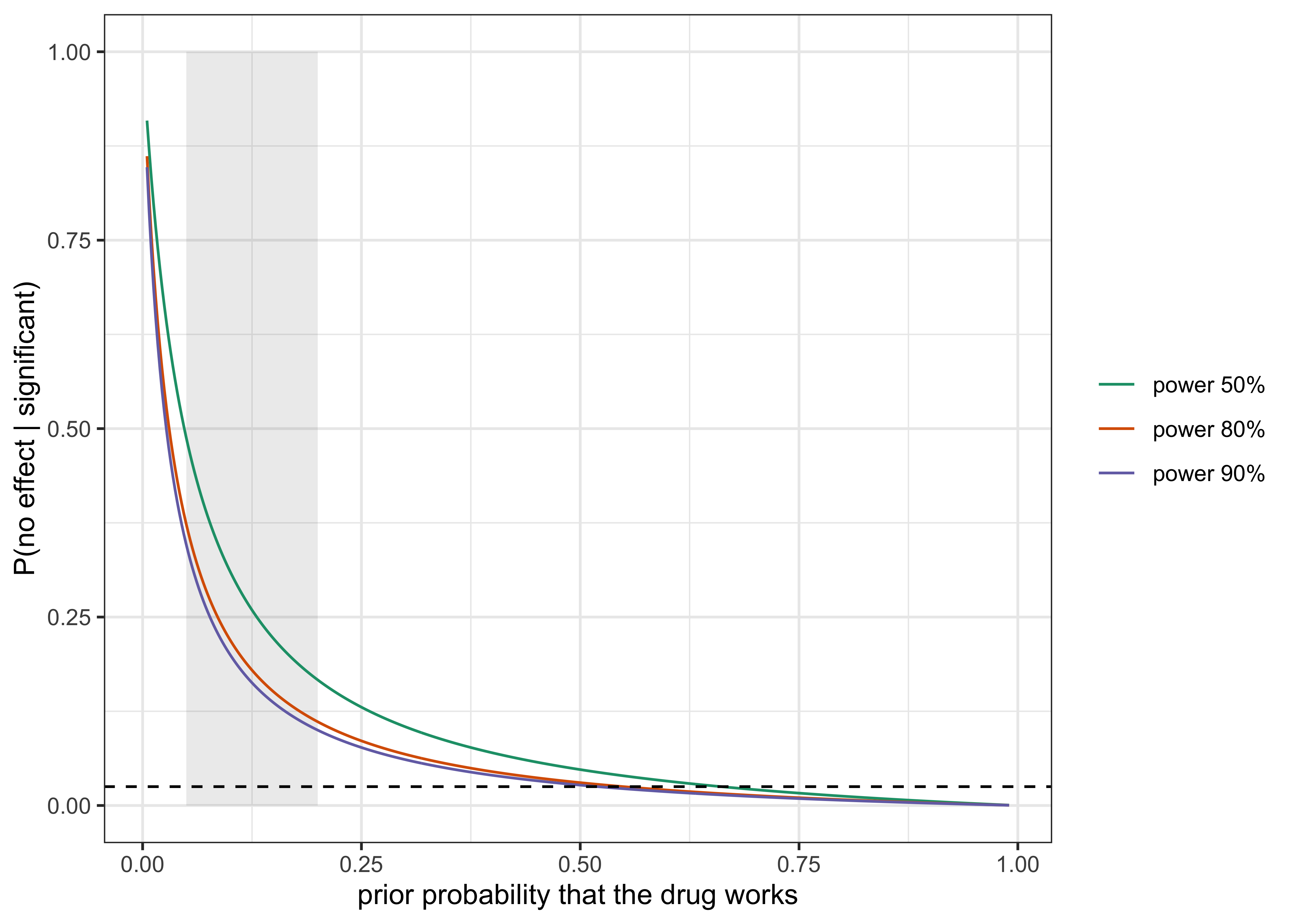
If half of all drugs entering a confirmatory trial work, a significant result at one-sided 0.025 with 90% power is wrong about 2.7% of the time, close to the nominal 0.025. If one in ten works, the false positive risk after a significant result is 20%, eight times the nominal level. If one in a hundred works, which is not an absurd figure for an early-stage mechanism with a poor track record, a significant result is more likely to be false than true even with a well-powered trial: 73% (Figure 7.1 plots the whole curve).

Two practical lessons follow. First, power is not only about not missing a real effect; it also protects against false positives, because the denominator of Equation 7.1 contains \((1-\beta)\pi_a\). An underpowered trial that happens to cross the line is more likely to have done so by chance. Second, the same type I error level means different things in different development programs. A phase 3 trial confirming a dose chosen after two positive phase 2 studies sits at the top of Table 7.1. A trial of a novel mechanism in a disease with a long record of failures sits near the bottom. The empirical record bears this out: in a review of phase III oncology trials that repeated a regimen already positive in phase II, only 28% were themselves positive (Zia et al. 2005) (Section 7.10). The regulator’s decision to demand two trials, or one trial and confirmatory evidence (the FDA substantial-evidence draft, see Chapter 3), can be read as a way of pushing the prior probability of a true effect up before approval, and thus pushing the false positive risk down.

p_works <- seq(0.005, 0.99, length.out = 400)
d <- do.call(rbind, lapply(c(0.9, 0.8, 0.5), function(pw)
  data.frame(p_works = p_works, fpr = false_positive_risk(p_works, pw), power = paste0("power ", 100 * pw, "%"))))
ggplot(d, aes(p_works, fpr, colour = power)) + annotate("rect", xmin = 0.05, xmax = 0.20, ymin = 0, ymax = 1, alpha = 0.12) +
  geom_line() + geom_hline(yintercept = 0.025, linetype = 2) + scale_colour_brewer(palette = "Dark2") +
  labs(x = "prior probability that the drug works", y = "P(no effect | significant)", colour = NULL) + theme_bw()

Figure 7.1: False positive risk as a function of the prior probability that the drug works, for three levels of power. The dashed line is the nominal alpha = 0.025. The shaded band marks priors between 5% and 20%.

NoteWhat a sponsor should take from this

The false positive risk is not an alternative to the type I error rate. The type I error rate is \(\Pr(\text{significant} \mid \text{no effect})\) and is what a design controls. The false positive risk is \(\Pr(\text{no effect} \mid \text{significant})\) and is what a decision-maker wants. They are connected by the prior probability of an effect, and the Bayesian framework is the one that lets that prior enter the analysis openly instead of silently. In a regulatory submission, the prior still has to be defended (Chapter 8) and, for a confirmatory design without borrowing, this book calibrates it to a one-sided type I error of 0.025 (Chapter 14). Calibration is one of the routes the FDA draft describes, alongside direct interpretation of posterior probabilities and benefit-risk criteria, not a universal requirement.

7.3 The exact p-value and the Bayes factor

The false positive risk above conditions on “significant at \(\alpha\).” One can do better by conditioning on the actual data, and this requires comparing the null with a specific alternative.

The Bayesian measure of the evidence in the data for one hypothesis against another is the Bayes factor. For a null \(H_0:\theta = 0\) and an alternative \(H_1\) under which \(\theta\) has a prior distribution \(\pi(\theta)\),

\[ \mathrm{BF}_{10} \;=\; \frac{p(y \mid H_1)}{p(y \mid H_0)} \;=\; \frac{\int p(y \mid \theta)\,\pi(\theta)\,d\theta}{p(y \mid \theta = 0)}, \]

the ratio of the probabilities the two hypotheses assigned to the data that actually occurred. It updates prior odds into posterior odds:

\[ \underbrace{\frac{\Pr(H_1 \mid y)}{\Pr(H_0 \mid y)}}_{\text{posterior odds}} \;=\; \mathrm{BF}_{10} \times \underbrace{\frac{\pi_a}{\pi_0}}_{\text{prior odds}}, \tag{7.2}\]

where \(\pi_0\) and \(\pi_a\) are the prior probabilities of the null and the alternative. The notation is the book’s (see Appendix A); the sources in the Bayesian literature sometimes write the ratio the other way up, as \(\mathrm{BF}_{01}\), and the two are reciprocals.

Two things are worth noticing at once. The Bayes factor weighs the data against both hypotheses, which is what the p-value does not do. And it averages the likelihood under the alternative over the prior \(\pi(\theta)\), rather than evaluating it at the best-fitting \(\hat\theta\). This averaging is where the Bayes factor differs most from the likelihood ratio statistic familiar from frequentist testing, and it is where its penalty for vague alternatives comes from.

A Gaussian example with closed form

To keep the algebra short, work on the scale where the data reduce to the estimate \(\hat\theta_n\) with \(\hat\theta_n \mid \theta \sim N(\theta, 1/I_n)\), so that \(Z_n = \hat\theta_n \sqrt{I_n}\) is the usual standardized statistic and \(I_n\) is the Fisher information after \(n\) observations (for a time-to-event endpoint with \(d\) events and \(\theta = -\log\mathrm{HR}\), \(I_n \approx d/4\)). Take the alternative to be \(\theta \sim N(0, \tau^2)\), a prior centered at no effect with scale \(\tau\) that expresses how large an effect is plausible. Then the integral can be done exactly. With \(k = I_n \tau^2\) (the information in the data relative to the information in the prior),

\[ \mathrm{BF}_{10} \;=\; (1 + k)^{-1/2} \exp\!\left\{\tfrac12 Z_n^2 \,\frac{k}{1+k}\right\}, \qquad 2 \log \mathrm{BF}_{10} \;=\; Z_n^2 \,\frac{k}{1+k} \;-\; \log(1+k). \tag{7.3}\]

This is the form given by Polson and Sokolov (Polson and Sokolov 2026), and it is the finite-sample version of the Schwarz criterion (Schwarz 1978). For large \(k\) the factor \(k/(1+k)\) tends to one and

\[ 2 \log \mathrm{BF}_{10} \;\approx\; \underbrace{Z_n^2}_{\text{fit}} \;-\; \underbrace{\log(1+I_n\tau^2)}_{L_n,\ \text{Ockham penalty}}. \tag{7.4}\]

Read Equation 7.4 as a ledger. The first term is how well the best-fitting alternative explains the data, in standardized squared units, and it is the same quantity that the z test examines. The second term is a charge for flexibility. An alternative that spreads its prior over a wide range of effects \(\theta\) gives most of that range to effects that the data rule out, so on average it predicts the data worse than a sharp alternative would. The more data we collect (the larger \(I_n\)), the more sharply the data pin down \(\theta\), and the larger the share of the prior that is wasted: the penalty grows like \(\log I_n\). This is the Ockham penalty, the automatic, parameter-free version of “do not prefer a more complex hypothesis unless the data pay for it.”

The practical content for a trial: with \(\tau = 0.25\) on the log hazard ratio scale and \(I_n = 400\) (about 1,600 events), the penalty is \(L_n = \log(26) = 3.26\). The Bayes factor reaches 1 only when \(Z_n^2 \approx 3.26\), that is \(|Z_n| \approx 1.8\), and requires more than that for any substantial evidence. The p-value at \(|Z_n| = 1.8\) is 0.036 one-sided, which is not “significant” at 0.025 and yet is, on this measure, only just break-even evidence for the alternative.

Lindley’s paradox

Lindley (D. V. Lindley 1957), following Jeffreys (Jeffreys 1939) and Bartlett’s reply (Bartlett 1957), noticed that the penalty can turn a rejection of the null into evidence for the null (the Jeffreys-Lindley paradox). Consider a sequence of trials of increasing size, every one of which ends with the same two-sided p-value of exactly 0.01, so that \(|Z_n| = 2.576\) in every case. A frequentist reading says the evidence against the null is the same in each trial: significant at 1%. The Bayes factor says something else, because the Ockham penalty keeps growing while \(Z_n^2\) is stuck at 6.63.

z <- qnorm(1 - 0.005); tau <- 0.25
n <- c(10, 100, 1e3, 1e4, 1e5, 1e6)
lb <- bf10_normal(z, n * tau^2, log = TRUE)
knitr::kable(data.frame(n = n, BF10 = exp(lb), `P(H0 | data)` = posterior_null(lb, 0.5), check.names = FALSE), digits = c(0, 2, 3))

Table 7.2: Lindley’s paradox. Every row has the same two-sided p-value, 0.01 (z = 2.576). Prior N(0, 0.25^2) on the effect under the alternative, unit standard deviation per observation, prior probability of the null 0.5.

n	BF10	P(H0 | data)
1e+01	2.81	0.262
1e+02	6.48	0.134
1e+03	3.29	0.233
1e+04	1.10	0.477
1e+05	0.35	0.741
1e+06	0.11	0.901

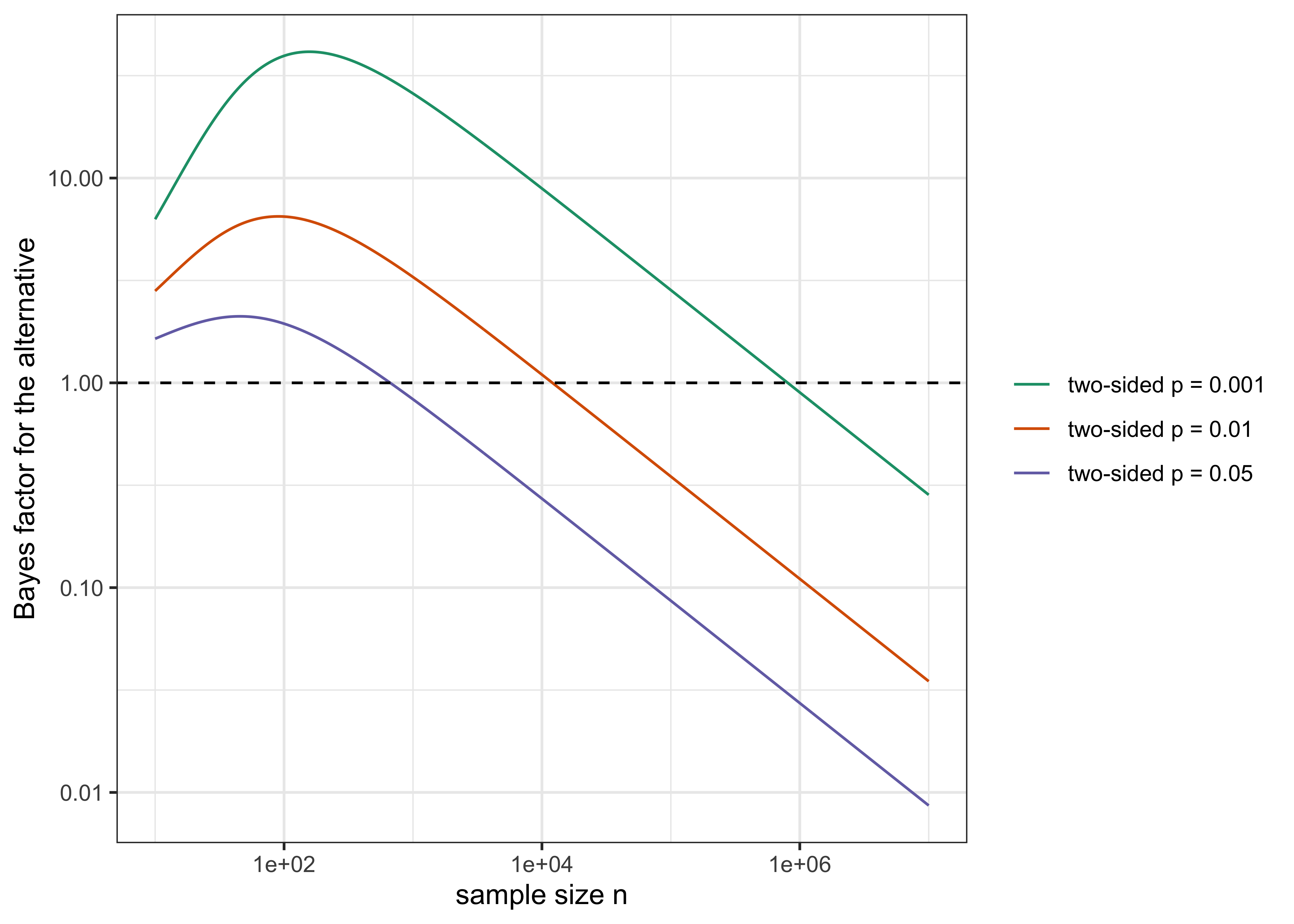
Table 7.2 and Figure 7.2 show the effect. At \(n = 100\) the Bayes factor is 6.5 in favor of the alternative, and the posterior probability of the null is 13%: not as small as the p-value of 0.01 suggests, but pointing the same way. By \(n = 10{,}000\) the Bayes factor is 1.1, the evidence is a wash, and the posterior probability of the null is 48%. At \(n = 10^6\) the same p-value of 0.01 corresponds to a posterior probability of the null of 90%. The data that “reject the null at the 1% level” have become strong evidence for it.

ns <- 10^seq(1, 7, length.out = 300)
d <- do.call(rbind, lapply(c(0.05, 0.01, 0.001), function(p2)
  data.frame(n = ns, bf = bf10_normal(qnorm(1 - p2 / 2), ns * tau^2), p = paste("two-sided p =", p2))))
ggplot(d, aes(n, bf, colour = p)) + geom_line() + geom_hline(yintercept = 1, linetype = 2) +
  scale_x_log10() + scale_y_log10() + scale_colour_brewer(palette = "Dark2") +
  labs(x = "sample size n", y = "Bayes factor for the alternative", colour = NULL) + theme_bw()

Figure 7.2: Lindley’s paradox. Holding the two-sided p-value at 0.01 (and also at 0.05 and 0.001), the Bayes factor for the alternative first rises and then falls as the sample size grows, crossing below 1 for large n. The dashed line is BF = 1.

How should a trialist react? There are two honest reactions and one dishonest one.

The honest reactions are these. First, the paradox lives at sample sizes far larger than those of most confirmatory trials of a large effect, and with a vague prior (\(\tau\) large) on a point null. It is a warning that a fixed p-value threshold cannot mean a fixed amount of evidence as the trial gets larger, which is why very large trials (cardiovascular outcome trials with tens of thousands of patients, platform trials with shared controls) sometimes find “significant” effects that are clinically trivial. The Bayesian remedy is a better question: instead of asking whether \(\theta\) is exactly zero, ask whether \(\theta\) exceeds a clinically relevant \(a\). That is precisely the form of the FDA’s criterion, as the last section of this chapter shows. Second, the paradox is a reminder that the answer depends on the prior \(\tau\) under the alternative. A Bayes factor with \(\tau\) ten times larger needs a much larger \(Z_n\) to reach the same conclusion. This sensitivity is real, it is not hidden by the frequentist approach but simply left out of it, and it is the reason Chapter 8 treats prior choice and sensitivity analysis at length.

The dishonest reaction is to pick \(\tau\) after seeing the data to give the result you want. A Bayes factor is as open to that abuse as a p-value is to choosing the test statistic after the fact, and the remedy is the same: pre-specify it in the protocol.

Edwards, Lindman and Savage (Edwards, Lindman, and Savage 1963) gave lower bounds over all priors on the alternative, showing that a result significant at 5% is weak evidence against a point null at any sample size, and Berger and Sellke (Berger and Sellke 1987) sharpened the point with lower bounds on the posterior probability of a point null over classes of priors, the Sellke-Bayarri-Berger bound used in the next section. Jeffreys, who developed the posterior-odds test of a point null in the 1930s (Jeffreys 1935) and set it out in his book (Jeffreys 1998) (the Oxford reprint of the third edition), wrote that the use of the p-value implies that “a hypothesis that may be true may be rejected because it has not predicted observable results that have not occurred”.

7.4 How small can the Bayes factor be? Calibrating the p-value

The Bayes factor depends on the prior under the alternative. Can we say anything that does not? Yes, at the cost of being deliberately generous to the alternative. For any prior on the alternative, the Bayes factor against the null cannot be larger than what the most favorable choice produces. Sellke, Bayarri and Berger (Sellke, Bayarri, and Berger 2001) showed that for a p-value \(p < 1/e\) and for a class of alternatives (the p-value is uniformly distributed under the null, and under the alternative the distribution of \(-\log p\) has a non-increasing hazard for \(Y = -\log p\) (their Section 3.1.3), of which the Beta\((\xi, 1)\) family of p-value densities is the leading example), the Bayes factor in favor of the null is at least

\[ \mathrm{BF}_{01} \;\ge\; -e\, p \log p. \tag{7.5}\]

This is a minimum Bayes factor, a bound on how strongly the data can favor the alternative within that class. The class matters: monotonicity of the p-value density alone is not enough, and the bound is not a statement about every prior. For \(Z \sim N(\theta, 1)\) with \(Z = 1.96\) and prior mass one half at each of \(\theta = \pm 1.96\), the Bayes factor in favor of the null is about 0.29, below the bound of 0.41 at \(p = 0.05\). The bound calibrates a p-value against the stated class, and it should be quoted with that qualification. Combined with prior odds on the null of one to one (\(\pi_0 = \pi_a = 0.5\)), it gives a lower bound on the posterior probability of the null:

\[ \Pr(H_0 \mid y) \;\ge\; \left(1 + \frac{1}{-e\,p\log p}\right)^{-1}. \]

p <- c(0.10, 0.05, 0.025, 0.01, 0.005, 0.001)
b01 <- min_bf(p, type = "pvalue")
knitr::kable(data.frame(`two-sided p` = p, `min BF01` = b01, `max BF10` = 1 / b01,
  `min P(H0|data)` = b01 / (1 + b01), check.names = FALSE), digits = c(3, 3, 1, 3))

Table 7.3: Calibration of two-sided p-values by the Sellke-Bayarri-Berger bound. ‘Max BF10’ is the largest Bayes factor for the alternative that any member of the class can produce. ‘Min P(H0 | data)’ assumes prior probability 0.5 on the null.

two-sided p	min BF01	max BF10	min P(H0|data)
0.100	0.626	1.6	0.385
0.050	0.407	2.5	0.289
0.025	0.251	4.0	0.200
0.010	0.125	8.0	0.111
0.005	0.072	13.9	0.067
0.001	0.019	53.3	0.018

A two-sided p-value of 0.05 corresponds at best to a Bayes factor of about 2.5 for the alternative, and to a posterior probability of the null of at least 29% if the null and alternative were equally likely at the outset. So the “5% significance” that is so often read as “95% sure” is, from this angle, at best “71% sure.” A p-value of 0.01 corresponds to a Bayes factor of at most 8 and a posterior probability of the null of at least 11%. Only at \(p = 0.001\) does the bound get to the neighbourhood of “strong evidence” (a Bayes factor of 53). This is the calculation behind the teal bar in module 2 of the companion lab (“the smallest chance that luck alone could still explain the result, given that p-value, assuming a 50:50 chance before the trial”). It is also an argument that has been made for tightening the default threshold for claims of new discoveries (Benjamin et al. 2018), a proposal that is controversial and does not apply to regulatory trials, where the one-sided 0.025 is set by decades of agency practice and by the substantial-evidence standard, not by a statistician’s preference.

What the bound does not do is replace a design-specific calculation. It is generous to the alternative within its class (it asks which alternative would make the data look best for \(H_1\)), so it understates what a reasonable analysis would find. In a trial, the prior under the alternative comes from the phase 2 data, the mechanism, and the effect size the trial was powered for, and Chapter 8 and Chapter 14 show how to build and defend it.

The bound is a best case over a class of alternatives. A different route to the same kind of calibration fixes a Bayes factor threshold and asks which test reaches it most often. Johnson’s uniformly most powerful Bayesian tests (Johnson 2013b) choose, for a one-parameter exponential family such as a normal mean, the alternative that maximizes the probability that the Bayes factor exceeds a stated threshold, and their link to classical uniformly most powerful tests gives an approximate calibration between p-values and Bayes factors. Johnson used it to argue for tighter standards of evidence (Johnson 2013a), a proposal in the direction of Benjamin and colleagues’ 0.005 (Benjamin et al. 2018). Cornfield (Cornfield 1966) put a prior probability on the null in a Bayesian sequential test for clinical trials, and Kass and Raftery (Kass and Raftery 1995) give the scale on which such Bayes factors are usually read. Goodman’s two papers (S. N. Goodman 1999a, 1999b) explain to clinicians why a p-value is not the probability that the null is true and how a Bayes factor answers a different question. What the two bars of Section 7.5.1 add is that the threshold is not fixed: for a normal mixture alternative the Bayes factor bar grows with the information, so no single p-value cutoff corresponds to one Bayes factor as a trial grows.

7.5 One toll, three scales: how much evidence is enough?

The Ockham penalty in Equation 7.4 says that a Bayesian who uses a point null and a diffuse alternative has to see more than a one-sided z test’s \(Z_n^2 = 1.96^2 = 3.84\) before acting once the information is large (for a one-sided claim, with \(Z_n > 0\)). The following is the first part of the framework in Polson and Sokolov’s working paper (Polson and Sokolov 2026); the rest of it appears in later chapters, as flagged below.

A reader may object that tuning a Bayesian rule until its type I error is 0.025 gives up the Bayesian position. Frequentist evaluation of Bayesian procedures has a long applied tradition. Rubin argued that the applied statistician should use Bayesian methods to build procedures and frequency calculations to judge them (Rubin 1984). Lewis and Berry applied exactly that program to clinical trials, judging Bayesian decision-theoretic designs by their classical operating characteristics (Lewis and Berry 1994), and Grieve’s “idle thoughts of a well-calibrated Bayesian” bring the argument to drug development and discuss how closely Bayesian procedures should match conventional frequentist targets (Grieve 2016). Dawid’s forecast-calibration result, that a coherent forecaster should expect to be well calibrated against the frequencies of the events forecast, concerns a different property than fixed-null type I error control (Dawid 1982). Evaluating a Bayesian procedure by its frequentist behavior is therefore Bayesian practice and not a compromise with the other school, and it is what the regulator asks for when the design is calibrated.

The two bars

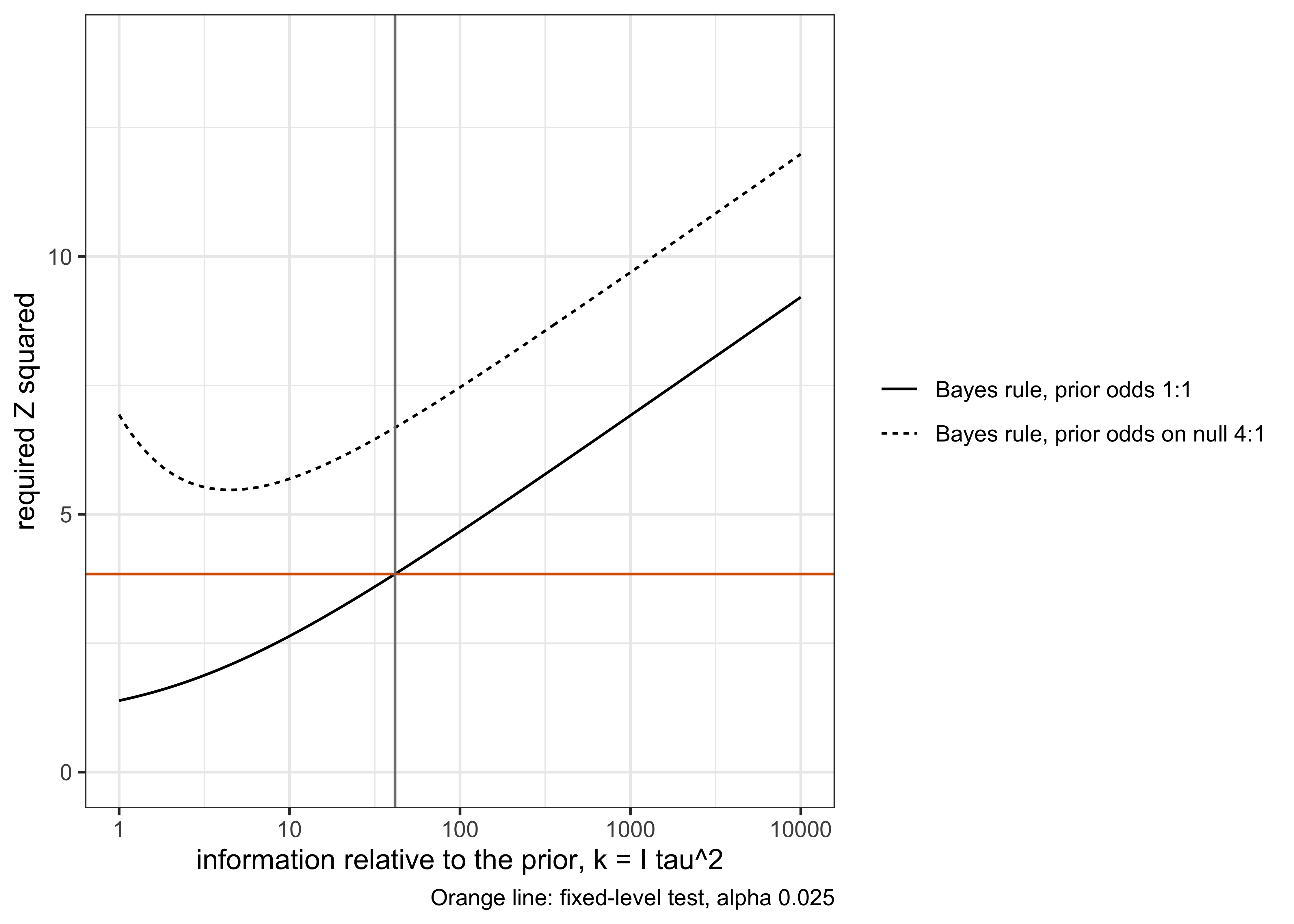
In plain terms: a fixed-level one-sided test acts when \(Z_n \ge z_\alpha\), equivalently (for \(Z_n > 0\)) when \(Z_n^2\) passes a constant bar, 3.84 at one-sided \(\alpha = 0.025\), whatever the sample size. A Bayes rule that acts when the alternative is at least as probable as the null passes a bar that grows with the logarithm of the information, plus a constant that is positive when the null is favored at the outset. At small samples the Bayes bar is the lower one, at large samples it is the higher one, and whether a given trial is past the point where they cross depends on the prior scale. The comparison is for the specified uncalibrated point-null rule with a symmetric normal alternative. Figure 7.3 shows the two bars, and the note below derives them.

NoteTechnical note: the two bars and where they cross

A decision rule that says “act when the evidence passes a bar” can be written as a condition on \(Z_n^2\), together with the positive-direction condition \(Z_n > 0\) when the claim is one-sided (the symmetric Bayes factor measures departure in either direction). Two rules, and what each charges:

• The fixed-level test acts when \(Z_n \ge z_\alpha\), that is, when \(Z_n > 0\) and \(Z_n^2 \ge z_\alpha^2\). The bar on \(Z_n^2\) is a constant: 3.84 at one-sided \(\alpha = 0.025\), whatever the sample size. This is the traditional rule, calibrated to a type I error rate that does not depend on \(n\).
• The Bayes rule acts when the posterior odds in favor of the alternative reach one, \(\pi_a \mathrm{BF}_{10} \ge \pi_0\) (act when the alternative is at least as probable as the null, which is optimal if wrongly acting and wrongly not acting cost the same). By Equation 7.2 this is \(\mathrm{BF}_{10} \ge \pi_0/\pi_a\), and by Equation 7.4 it is, in the large-information approximation and with \(Z_n > 0\) for a one-sided claim,

\[ Z_n^2 \;\ge\; L_n + C, \qquad L_n \sim \log n, \qquad C = 2\log\frac{\pi_0}{\pi_a}. \tag{7.6}\]

The exact bar for the normal mixture of Equation 7.3 carries the factor \((1 + 1/k)\): \(Z_n^2 \ge (1 + 1/k)\,(L_n + C)\) with \(k = I_n\tau^2\). The bar of the Bayes rule is not constant. It grows with the logarithm of the sample size (more precisely, of the information \(I_n\tau^2\)), plus a constant \(C\) that is zero if the null and the alternative are equally probable a priori, positive if the null is favored (the usual case for a drug that has to prove itself), and negative if the alternative is favored.

Each bar is a price. The fixed-level test charges a flat \(z_\alpha^2\). The Bayes rule charges \(\log n + C\), which at small \(n\) is less than the flat price and at large \(n\) is more. Where do they cross? Set \(\log n + C = z_\alpha^2\) (asymptotically). With \(C = 0\) and \(\alpha = 0.025\),

\[ n^\ast \;=\; e^{z_\alpha^2} \;=\; e^{3.84} \;\approx\; 46. \tag{7.7}\]

Here \(n\) is measured in units of the prior’s information, so that \(L_n = \log(1 + I_n\tau^2) \approx \log n\). The exact Gaussian expression of Equation 7.3 gives the crossing at \(I_n\tau^2 = 41.6\), close to the asymptotic 46. In plain terms: once the data carry about forty to fifty times the information in the prior, the uncalibrated point-null Bayes rule asks for more than the fixed-level test does. Whether a given trial is past that point depends on the prior scale. For a prior of \(\tau = 0.25\) on the log hazard ratio, the asymptotic crossing of 46 corresponds to \(I_n > 730\) and about 2,900 events (the exact 41.6 gives 666 and about 2,660), the size of a large cardiovascular outcome trial and not of every confirmatory trial; the example of this section, with \(I_n\tau^2 = 25\), is below the crossing. For a prior with a larger \(\tau\) the crossing arrives sooner, and for a smaller \(\tau\) later.

k <- 10^seq(0, 4, length.out = 400); z2 <- qnorm(0.975)^2; kc <- crossing_n()
d <- data.frame(k = rep(k, 2), bar = c(bayes_bar(k, 1), bayes_bar(k, 4)),
  rule = rep(c("Bayes rule, prior odds 1:1", "Bayes rule, prior odds on null 4:1"), each = length(k)))
ggplot(d, aes(k, bar, linetype = rule)) + geom_line() + geom_hline(yintercept = z2, colour = "#D95F02") +
  geom_vline(xintercept = kc, colour = "grey50") + scale_x_log10() + coord_cartesian(ylim = c(0, 14)) +
  labs(x = "information relative to the prior, k = I tau^2", y = "required Z squared", linetype = NULL,
       caption = "Orange line: fixed-level test, alpha 0.025") + theme_bw()

Figure 7.3: The first two tolls. The fixed-level test acts when Z squared exceeds the constant 3.84 (one-sided alpha 0.025). The Bayes rule with prior odds 1 to 1 acts when Z squared exceeds the Ockham bar, which grows like the logarithm of the information. The two cross where the information is about 42 times the prior information. The dotted curve shows the bar when the prior odds on the null are 4 to 1 (C = 2 log 4).

Two consequences for the reader who runs trials.

The Bayesian bar is not lower. A recurring claim is that Bayesian trials “need less evidence.” Against a single unadjusted look at a fixed-level test, the opposite holds for the uncalibrated point-null rule once information times prior variance exceeds about 46 (exactly, about 41.6; a few dozen observations for a unit-information prior, far more at the prior scales used for hazard ratios): the Bayes rule with a point null charges more. A Bayesian bar calibrated to the same type I error is never lower at a single look without an informative prior. The gains of Bayesian adaptive designs come from elsewhere, namely monitoring, multiple arms and prior information, and each is costed later in the book (Chapter 11, Chapter 10, Chapter 19). This is the thesis of the book and it is first visible in Equation 7.7.

A third toll exists, and it is the one that matters for monitoring. Both bars above are for a decision made once, at a pre-specified sample size. If the trial is looked at repeatedly and one wants the type I error to hold at every stopping time, the bar has to rise again. For the symmetric normal-mixture e-process of this chapter, comparing the threshold \(b = 1/\alpha\) with the baseline \(b = 1\), the increase in the squared-\(Z\) bar is \(2\log(1/\alpha)(1 + 1/k)\), which tends to the constant \(2\log(1/\alpha) = 7.38\) at \(\alpha = 0.025\) as the information grows. This is the anytime-valid surcharge for this construction, and it comes from Ville’s inequality for test martingales. It is a large-information approximation for this normal mixture, not a universal minimum cost of sequential validity: other e-processes, such as those behind iterated-logarithm confidence sequences, behave differently. It is developed in Chapter 12, and the sequential story, where the three tolls \(z_\alpha^2\), \(\log n\) and \(\log n + 2\log(1/\alpha)\) become the three deviation scales and meet the group sequential boundaries (Pocock, O’Brien-Fleming, Lan-DeMets), is told in Chapter 11.

NoteTechnical note: why log n, and where the constant C comes from

Under the Gaussian model, the evidence that \(\theta\) is nonzero accumulates in the statistic \(S_n = \hat\theta_n I_n\), which behaves like Brownian motion in information time with drift \(\theta\). The Bayes factor of Equation 7.3 integrates the exponential likelihood ratio over the prior. A Laplace approximation of that integral gives the maximized log likelihood ratio, \(Z_n^2/2\), minus the log of the ratio of the prior’s width to the posterior’s width, \(\tfrac12\log(1 + I_n\tau^2)\). The posterior width shrinks like \(I_n^{-1/2}\), so the ratio grows like \(I_n^{1/2}\) and its logarithm like \(\tfrac12 \log I_n\). Doubling gives the \(L_n\) of Equation 7.4.

For the constant, the Bayes rule for a two-point decision with equal costs acts when the posterior probability of the alternative exceeds one half, that is, when \(\mathrm{BF}_{10}\,\pi_a/\pi_0 \ge 1\). Taking logarithms, \(2\log \mathrm{BF}_{10} \ge 2\log(\pi_0/\pi_a)\), and substituting Equation 7.4 gives Equation 7.6. If the costs of the two errors differ, \(C\) absorbs their ratio as well. A regulator’s preference for protecting the public from false approvals can be written as a larger \(C\).

Setting \(b\) in “act when \(\mathrm{BF}_{10} \ge b\)” to \(1/\alpha\) turns the Bayes factor into an e-value test and gives the anytime-valid bar, exactly \((1 + 1/k)(L_n + 2\log(1/\alpha))\) and approximately \(L_n + 2\log(1/\alpha)\) for large information, discussed in Chapter 12. The Bayes rule at \(b = 1\) and the anytime-valid rule at \(b = 1/\alpha\) are built on the same statistic and differ only in where the bar is placed.

What this means for the protocol

A protocol written in the traditional style states a fixed-level test and a sample size computed from it. A protocol with a Bayes factor decision (rare in confirmatory trials, more common in early phase and in decision-theoretic designs) states the prior under the alternative, the prior odds or threshold, and the resulting bar. The table below compares the two on the same trial; the regulator’s question for either is the same one, namely what the operating characteristics are.

	Fixed-level z test	Bayes factor rule
Quantity compared with a bar	\(Z_n\) against \(z_\alpha\) (\(Z_n^2\) against \(z_\alpha^2\) when \(Z_n > 0\))	\(\mathrm{BF}_{10}\) against \(\pi_0/\pi_a\), or \(Z_n^2\) against \(L_n + C\)
Bar depends on \(n\)?	No	Yes, like \(\log n\)
Needs a prior?	No	Yes: \(\tau\) and \(\pi_0/\pi_a\)
Type I error	\(\alpha\), by construction	Falls with \(n\); must be computed by simulation for the actual design
Where it agrees	One-sided p-value \(<0.025\)	At the crossing \(n^\ast\), where the two bars are equal
What the regulator asks	Is \(\alpha\) spent correctly?	What are the operating characteristics, and why this prior?

7.6 A test is a Bayes rule for an implied loss

The previous section priced evidence with a bar. This section asks what a bar is worth, and the answer ties the chapter back to the type I error and power of Chapter 4. The frequentist ledger holds two numbers, the type I error \(\alpha\) and the power \(1-\beta_\theta\) at each effect \(\theta\), each computed with the parameter held fixed. The Bayesian ledger holds one, the Bayes risk, which weighs the same two errors by how likely each state of the world is and by how much each mistake hurts. The two ledgers are not rivals: one is built from the other.

The Bayes risk of a test

Let \(D(y) = 1\) declare the treatment effective. Let \(\pi_0 = \Pr(H_0)\), let the effect have density \(g(\theta)\) under \(H_1\), and let the loss be \(\ell_1\) for approving a useless drug and \(\ell_0\) for withholding a useful one (zero otherwise). The Bayes risk of \(D\) is its expected loss over both the parameter and the data,

\[ r(D) \;=\; \pi_0\,\ell_1\,\alpha(D) \;+\; (1-\pi_0)\,\ell_0 \int \beta_\theta(D)\, g(\theta)\, d\theta . \tag{7.8}\]

A frequentist who reports \(\alpha\) and \(\beta\) has reported the ingredients of the risk, and the weights are what is missing: the prior probability of each state times the loss of the corresponding mistake. The rule that minimizes \(r(D)\) is found one data set at a time. For each \(y\) the contribution to the risk is linear in \(D(y) \in \{0, 1\}\), so the optimal rule picks the action with the smaller coefficient, which gives

\[ D^{B}(y) = \mathbf 1\{\mathrm{BF}_{10}(y) > b\}, \qquad b = \frac{\pi_0}{1-\pi_0}\cdot\frac{\ell_1}{\ell_0}, \tag{7.9}\]

equivalently, reject when the posterior probability of \(H_0\) falls below \(\ell_0/(\ell_0 + \ell_1)\). This is the rule for choosing between a point null and a symmetric alternative, with its threshold read as a loss ratio, and it uses only the data that occurred. It is two-sided model selection: the alternative \(N(0,\tau^2)\) puts mass on harmful effects, so \(\Pr(H_1\mid y)\) is not the benefit probability \(\Pr(\theta>a\mid y)\) of the FDA criterion in Equation 7.11. A rule for approving on benefit needs hypotheses and losses that separate beneficial from harmful effects, and restricting this rule to \(Z_n>0\) does not preserve its optimality. The averaging over data that did not occur defines the risk it minimizes, but it is not needed to find the rule.

The Neyman-Pearson lemma (Neyman and Pearson 1933) is a statement about the same rules. Minimizing the type II error at a simple alternative \(\theta_1\) subject to \(\alpha(D) \le \alpha\) is the same as minimizing \(\beta_{\theta_1}(D) + \lambda\,\alpha(D)\) for some multiplier \(\lambda \ge 0\), which is the Bayes risk with \(g\) a point mass, \((1-\pi_0)\ell_0 = 1\) and \(\pi_0 \ell_1 = \lambda\). So every most powerful test is a Bayes rule for some prior odds and loss ratio, and the likelihood-ratio cutoff \(k_\alpha\) is the product in Equation 7.9. A trialist who fixes \(\alpha\) has chosen this product without saying so. The useful question is how the implied choice behaves as the trial grows.

What a fixed level implies as information grows

Take the normal model of Equation 7.3, \(\theta \sim N(0, \tau^2)\) under \(H_1\), with \(q = I_n\tau^2\). The fixed-level test that acts when \(|Z_n| > z_{\mathrm{crit}}\) is exactly the Bayes rule \(\mathrm{BF}_{10} > b_n\) with

\[ 2\log b_n \;=\; z_{\mathrm{crit}}^2\,\frac{q}{1+q} - \log(1+q), \qquad\text{so}\qquad b_n \approx \frac{e^{z_{\mathrm{crit}}^2/2}}{\sqrt{q}} \to 0 . \tag{7.10}\]

The implied threshold is simply the Bayes factor at the boundary, so the first column of Table 7.4 is both the Lindley paradox at \(Z = 1.96\) and the implied Bayes-factor threshold of the 5% test (a two-sided point-null quantity, not a one-sided benefit bar). A regulator that holds \(\alpha\) fixed behaves, as trials grow, as if the prior odds on the null or the harm of a false approval were shrinking toward zero. Here the prior is the unit-information prior, \(\tau = 1\) on the scale of one observation, so \(q = n\); the table of Section 7.3.2 used \(\tau = 0.25\) and a p-value of 0.01, and the pattern is the same.

lt <- decide_lindley_table(n = c(10, 100, 1e3, 1e4, 1e5), z = 1.96, tau = 1)
knitr::kable(data.frame(n = lt$n, `Implied threshold = BF10 at Z = 1.96` = lt$B, `P(H0 | Z = 1.96)` = lt$post_null, check.names = FALSE), digits = c(0, 3, 2), format.args = list(big.mark = ","))

Table 7.4: A result on the conventional boundary, Z = 1.96, as the trial grows. Prior N(0, 1) on the effect (unit information, q = n), equal prior odds. The Bayes factor at the boundary is the Bayes-factor threshold implied by the 5% test (Equation 7.10); P(H0) is the posterior probability of the null.

n	Implied threshold = BF10 at Z = 1.96	P(H0 | Z = 1.96)
1e+01	1.728	0.37
1e+02	0.666	0.60
1e+03	0.215	0.82
1e+04	0.068	0.94
1e+05	0.022	0.98

At \(n\) = 10 a result on the boundary of significance mildly favors an effect (Bayes factor 1.73). At \(n\) = 100 it already favors the null (0.67), and at \(n\) = 1e+05 it corresponds to a posterior probability of the null of 0.98. The 5% test is a Bayes rule at every \(n\), but for an implied loss that drifts with \(n\).

The type I error of the Bayes rule

The converse question is what type I error the Bayes rule has. With equal odds and loss (\(b = 1\)), the exact bar on \(|Z_n|\) is \(\sqrt{(1 + 1/q)\log(1+q)}\), the bar of Equation 7.6 with the factor of the technical note above, so the type I error is \(2\{1 - \Phi(\text{bar})\}\). It exceeds 5% for small trials, passes 5% at the crossing \(q\) = 41.6 of Section 7.5.1, and falls thereafter, roughly like \((q \log q)^{-1/2}\) in the large-information approximation. Table 7.5 gives the exact values, with the Bayes risk of the two rules at \(\pi_0 = 1/2\) and equal losses (\(\ell_0 = \ell_1 = 1\)).

tb <- decide_bayes_type1_table(n = c(10, 100, 1e3, 1e4), tau = 1)
rk_fix <- decide_bayes_risk(b = 1.96, q = tb$q)
rk_bay <- decide_bayes_risk(b = tb$bar_exact, q = tb$q)
knitr::kable(data.frame(n = tb$n, `Bayes bar` = tb$bar_exact, `Type I error, Bayes rule` = tb$alpha_exact, `Risk, 5% test` = rk_fix$risk, `Risk, Bayes rule` = rk_bay$risk, check.names = FALSE), digits = c(0, 2, 4, 4, 4), format.args = list(big.mark = ","))

Table 7.5: The Bayes rule (BF10 > 1, equal prior odds, unit-information prior N(0, 1), q = n) against the fixed 5% test. The exact bar is sqrt((1 + 1/q) log(1 + q)). Risk is the Bayes risk of Equation 7.8 with pi0 = 0.5 and equal losses.

n	Bayes bar	Type I error, Bayes rule	Risk, 5% test	Risk, Bayes rule
10	1.62	0.1044	0.2477	0.2400
100	2.16	0.0309	0.1023	0.1005
1,000	2.63	0.0085	0.0497	0.0374
10,000	3.04	0.0024	0.0328	0.0133

The two rules have the same risk near the crossing and then separate. The fixed-level test has Bayes risk at least \(\pi_0\ell_1\alpha\) for every \(n\), because its type I error is \(\alpha\) at every \(n\). For the Bayes rule both error rates tend to zero, the type I error by the display above and the type II error at each \(\theta \neq 0\) because the statistic grows like \(\sqrt{n}\,\theta\) while the bar grows like \(\sqrt{\log n}\), so its risk tends to zero. A fixed bar spends a constant error forever, and by Lindley’s paradox the constant is spent on exactly the cases where the evidence favors the null. This is the point-null, two-sided calculation. The one-sided confirmatory rule of the protocol is a different decision problem, and deriving its Bayes rule needs hypotheses and losses that distinguish beneficial from harmful effects, which this section does not do.

Which error matters more

The threshold-as-loss-ratio derivation and its table are in Section 1.6; here only the prior odds enter the new part. By Equation 7.9, with equal prior odds, acting when \(\Pr(H_1 \mid y) > p^\star\) is optimal when a false approval is \(p^\star/(1-p^\star)\) times as costly as a false rejection, whatever the prior odds: with \(p^\star = \ell_1/(\ell_0+\ell_1)\) the prior odds are already inside the posterior, and they multiply only the Bayes-factor threshold \(b\).

lr <- decide_loss_ratio(pstar = c(0.975, 0.99, 0.995))
knitr::kable(data.frame(`Threshold p*` = lr$pstar, `Implied ratio l1/l0` = lr$ratio, check.names = FALSE), digits = c(3, 0))

Table 7.6: Posterior probability thresholds and the loss ratio they imply (false approval relative to false rejection).

Threshold p*	Implied ratio l1/l0
0.975	39
0.990	99
0.995	199

A threshold of 0.975 (which equals a one-sided 0.025 only under the flat-prior, normal, single-look conditions of Section 1.6, and which is a threshold on the benefit probability of a continuous model, not on \(\Pr(H_1\mid y)\) in the point-null model, so the two 0.975 thresholds are not interchangeable) therefore says that approving a useless drug is 39 times worse than withholding a useful one, 0.99 says 99, and 0.995 says 199. Writing the threshold as a loss ratio forces the question that a fixed \(\alpha\) hides: is a false approval in this indication really 100 or 200 times worse than a false rejection?

The ratio is not a statistical quantity. In a refractory cancer with no effective therapy, delay costs months of life and a false approval of a drug that does little harm costs relatively little, so the ratio is small and the threshold can be lower. For a preventive drug taken for years by millions of healthy people, a false approval exposes a large population to side effects for no benefit while delay costs each person little, so the ratio is large and the threshold should be higher. In a pandemic vaccine the cost of delay is counted in deaths per week, and the ratio is small even though the population is large. Isakov, Lo and Montazerhodjat (Isakov, Lo, and Montazerhodjat 2019) carry out this exercise across diseases with burden-of-disease data and find that the best threshold differs by disease, so that a single conventional \(\alpha\) cannot be the Bayes rule for all of them. A protocol that states its threshold with a loss ratio, and a reason, is more informative than one that states \(\alpha\) alone (the loss-ratio reading of a posterior threshold returns in Chapter 15).

The Jeffreys table, in terms of \(q\)

The growth of the bar is old. Jeffreys (Jeffreys 1939) derived it for a normal mean with the Cauchy prior he recommended on invariance grounds. To leading order in \(n\) the Bayes factor in favor of the null is \(K = \sqrt{\pi n/2}\,\exp(-t^2/2)\), which falls through one at \(t_{\mathrm{crit}} = \sqrt{\log(\pi n/2)}\). This is a large-information approximation, not an identity: evaluated exactly, the Cauchy Bayes factor at \(t_{\mathrm{crit}}\) is 1.30 at \(n = 10\) and 1.008 at \(n = 10^3\). Table 7.7 restates the criterion in terms of \(q\) and sets it beside the exact bar of the normal-mixture rule of Section 7.5.1, which is what the rest of the chapter uses.

jt <- decide_jeffreys_table(n = c(10, 1e2, 1e3, 1e4, 1e5, 1e6), tau = 1)
knitr::kable(data.frame(`q = n` = jt$q, `t_crit` = jt$t_crit, p = jt$p_two_sided, `t (K^-1 = 10)` = jt$t_strong, `Normal bar, BF = 1` = jt$bar_mix_1, `Normal bar, BF = 10` = jt$bar_mix_strong, Conventional = jt$conventional, check.names = FALSE), digits = c(0, 2, 4, 2, 2, 2, 2), format.args = list(big.mark = ","))

Table 7.7: Jeffreys’ criterion in standardized units, with unit prior scale so that q=n. t_crit is the large-information approximation to where the Cauchy-prior Bayes factor turns against the null (the exact crossing is somewhat higher at small n); p is its two-sided tail probability; t (K^-1=10) is the value for Jeffreys’ grade of strong evidence; the last two columns are the exact bar of the normal-mixture Bayes rule at BF10 = 1 and at BF10 = 10, and the conventional 1.96.

q = n	t_crit	p	t (K^-1 = 10)	Normal bar, BF = 1	Normal bar, BF = 10	Conventional
1e+01	1.66	0.0970	2.71	1.62	2.78	1.96
1e+02	2.25	0.0245	3.11	2.16	3.05	1.96
1e+03	2.71	0.0067	3.46	2.63	3.39	1.96
1e+04	3.11	0.0019	3.78	3.04	3.72	1.96
1e+05	3.46	0.0005	4.07	3.39	4.01	1.96
1e+06	3.78	0.0002	4.34	3.72	4.29	1.96

Two cautions keep the table from being misread. First, the bar is a function of the prior scale through \(q\), not of \(n\) alone. The Cauchy scale and the normal \(\tau\) are different priors (at \(q = 10\) the two bars in the table are approximately 1.66 and 1.62, the first being the asymptotic Cauchy threshold, whose exact crossing at \(n = 10\) is 1.83), and a prior concentrated on the small effects that cardiovascular trials target moves the same bar to much larger \(n\): with \(\tau = 0.25\) the rows read at \(q = n/16\), and the crossing with 1.96 arrives at the thousands of events found in Section 7.5.1, not at \(n \approx 30\). The statement that the fixed level is too lenient for every trial beyond a phase I cohort holds only for a unit-information prior. Second, the calculation prices a point null, and an exact zero effect is a convenience. Against an interval null of clinically negligible effects the dimensional penalties of the two continuous models can cancel, and the resulting bar depends on the interval and the priors chosen; no general growth rate is claimed here. Both cautions bear on how the bar should behave, which is why the prior scale and the odds belong in the protocol and not in a convention.

Lindley information and the Ockham penalty

Lindley (Dennis V. Lindley 1956) defined the information in an experiment as the expected reduction in entropy from prior to posterior, the mutual information between \(\theta\) and the data. For a normal mean with prior variance \(\tau^2\) and data of precision \(n/\sigma^2\) it is \(\tfrac12\log(1 + q)\), half of the Ockham penalty \(L_n = \log(1 + I_n\tau^2)\) that sets the Bayes bar. The coincidence is not an accident: the Bayes factor charges the alternative the amount of information that an experiment of this size could deliver about \(\theta\), and the bar rises like \(\log n\) because the information does. With \(\tau = 0.25\) and \(\sigma = 1\) a trial delivers 1.0, 1.9, 2.8, 3.8 bits at \(n = 50, 200, 800, 3200\): each quadrupling of the trial adds about one bit. Information returns are logarithmic, so the evidence a larger trial must clear grows only slowly, and so does what it buys.

7.7 From p-values to posterior probabilities of benefit

The Bayes factor compares two hypotheses. For most clinical purposes there is a more useful number: the posterior probability that the treatment effect is large enough to matter. Chapter 6 built the posterior distribution of \(\theta\); here the question is how to turn it into a go/no-go criterion that a regulator can accept.

The FDA’s success criterion

The January 2026 FDA draft guidance on the use of Bayesian methodology (U.S. Food and Drug Administration 2026), section IV.A, describes the standard way a Bayesian trial defines success. It says that Bayesian success criteria are typically “based on the posterior probability that the true treatment effect size exceeds some threshold.” In the notation of the guidance and of this book,

\[ \Pr(\delta > a \mid \text{data}) \;>\; c, \tag{7.11}\]

where \(\delta\) is the treatment effect, \(a\) is the threshold (a minimum clinically relevant benefit, or zero if any benefit counts) and \(c\) is the minimum posterior probability. The notation \(\delta\) is used when quoting the criterion; elsewhere the book writes \(\theta\) for the same quantity. Two dials, then. The threshold \(a\) says how big an effect counts. The probability \(c\) says how sure one must be that it is at least that big. For trials with an overall frequentist statistical analysis plan, the same guidance says the success criteria are “almost always” chosen so that the familywise type I error is no greater than 0.025, one-sided, and that “a and c can be chosen such that the overall FWER is controlled at a given level, typically 0.025 one-sided” (section IV.A.1). It also describes two other routes: direct interpretation of posterior probabilities (for example with borrowing, by agreement with FDA) and decision-theoretic or benefit-risk criteria (section IV.A.3). Section IV.A is thus clear that a Bayesian criterion is a rule whose operating characteristics are to be reported. Calibration to the one-sided 0.025 is one of FDA’s routes and this book’s default for confirmatory adaptive designs without borrowing; it is not presented as FDA’s universal requirement.

The flat-prior case: where Bayes and the p-value agree

The simplest instance connects the criterion to what the reader already knows. Let the estimate be \(\hat\theta \sim N(\theta, s^2)\), with standard error \(s = 1/\sqrt{I_n}\), and let the prior on \(\theta\) be flat. The posterior is \(N(\hat\theta, s^2)\), so

\[ \Pr(\theta > a \mid \hat\theta) \;=\; \Phi\!\left(\frac{\hat\theta - a}{s}\right). \]

For the threshold \(a = 0\), this is \(\Phi(Z_n)\), which is exceeded by \(c = 0.975\) exactly when \(Z_n > 1.96\), that is, exactly when the one-sided p-value is below 0.025. A flat-prior posterior probability of benefit is one minus the one-sided p-value. The two numbers differ in how they are read (probability about the effect, given the data; probability of the data, given no effect), but the posterior probability is one minus the one-sided p-value, so the two thresholds agree and a trial that succeeds by one succeeds by the other. This is a useful cross-check to keep in the SAP: whatever a Bayesian analysis with a very weak prior reports, it should be close to the frequentist analysis of the same trial. It is also why the passage of Chapter 6 on credible intervals matches the confidence interval of the CSR to the second decimal for large trials.

The mapping from \((a, c)\) to type I error

With a flat prior, the criterion \(\Pr(\theta > a \mid \hat\theta) > c\) is equivalent to \(\hat\theta > a + z_c\, s\), where \(z_c = \Phi^{-1}(c)\). At \(\theta = 0\) (no effect) the probability that a trial meets the criterion is

\[ \alpha(a, c) \;=\; 1 - \Phi\!\left(\frac{a}{s} + z_c\right). \tag{7.12}\]

It follows that:

• With \(a = 0\), \(\alpha = 1 - c\). A criterion of \(c = 0.975\) gives \(\alpha = 0.025\). A criterion of \(c = 0.95\) gives 0.05, one-sided.
• With \(a > 0\), the type I error is smaller than \(1 - c\), because clearing a positive threshold is harder. To keep \(\alpha = 0.025\) at \(\theta = 0\) one can lower \(c\): the calibrating value is \(c = \Phi(z_{\alpha} - a/s)\). Lowering \(c\) in this way controls the error under the null \(\theta \le 0\), not under \(\theta \le a\): with \(a = s = 0.1\) the calibrating \(c \approx 0.83\) gives about 17% rejection at \(\theta = a\). The larger the threshold \(a\) is relative to the standard error, the lower \(c\) can be while the type I error stays at 0.025. When \(a\) is large compared with \(s\) one can end up at a \(c\) of 0.8 or so, a figure that looks lenient. This calibration reproduces the ordinary zero-null test: the rejection condition reduces to \(\hat\theta > z_\alpha s\) whatever \(a\) is, so it establishes superiority over zero, not benefit exceeding \(a\). To support a claim that the effect exceeds \(a\), calibrate at \(\theta = a\); in this flat-prior normal model that gives \(c = 0.975\). FDA draft section IV.A.1 uses \(a = 0\) for calibrated superiority designs.
• The calibration depends on \(s\), that is, on the sample size. A given pair \((a, c)\) gives a different \(\alpha\) in a trial with 200 patients than in one with 2,000.

s <- 0.10; a <- c(0, 0.05, 0.10, 0.15, 0.20)
knitr::kable(data.frame(a = a, `a/s` = a / s, `alpha at c=0.975` = type1_posterior_flat(a, 0.975, s),
  `alpha at c=0.90` = type1_posterior_flat(a, 0.90, s), `c giving alpha=0.025` = calibrate_c_flat(a, s),
  check.names = FALSE), digits = c(2, 2, 4, 4, 3))

Table 7.8: Mapping the posterior criterion Pr(theta > a | data) > c to the one-sided type I error at theta = 0 and to the calibrating c, for a flat prior. The standard error is s = 0.10 (so a/s is the threshold in standard errors). Calibration target: one-sided 0.025.

a	a/s	alpha at c=0.975	alpha at c=0.90	c giving alpha=0.025
0.00	0.0	0.0250	0.1000	0.975
0.05	0.5	0.0069	0.0374	0.928
0.10	1.0	0.0015	0.0113	0.831
0.15	1.5	0.0003	0.0027	0.677
0.20	2.0	0.0000	0.0005	0.484

In Table 7.8, with \(a = 0\), \(c = 0.975\) gives exactly 0.025; \(c = 0.90\) gives 0.10. When the threshold rises to one standard error (\(a = 0.10\)), the \(c = 0.975\) rule has a type I error of 0.0015, so it is much stricter than needed, and the calibrating \(c\) falls to 0.83. At two standard errors it falls to 0.48, close to a coin flip: a threshold of two standard errors above zero is itself about as demanding as the frequentist boundary, so little extra probability is needed on top of it. The numbers illustrate why guidance asks for calibration by simulation rather than by a rule of thumb about \(c\): the pair \((a, c)\) means nothing until it is attached to a sample size and a model.

An informative prior changes the mapping

A flat prior is the exception. The point of a Bayesian design is often to use prior information, or at least a skeptical prior that shrinks the estimate toward zero. With a prior \(\theta \sim N(0,\tau^2)\) the posterior is normal with mean \(w\hat\theta\) and variance \(w s^2\), where \(w = \tau^2/(\tau^2 + s^2)\) is the weight on the data. The criterion becomes \(\hat\theta > (a + z_c\sqrt{w}\, s)/w\), and a skeptical prior therefore raises the bar on \(\hat\theta\) at a given \(c\): the trial must show a larger observed effect to convince a skeptic. The type I error at \(\theta = 0\) falls, and so does the power.

tau <- c(100, 0.2, 0.1)
knitr::kable(data.frame(prior = c("flat (tau = 100)", "skeptical tau = 0.2", "skeptical tau = 0.1"),
  `type I error` = type1_posterior_normal(0, 0.975, 0.1, tau), `power at 0.3` = power_posterior_normal(0, 0.975, 0.1, tau, 0.3),
  `c for alpha=0.025` = calibrate_c_normal(0, 0.1, tau), check.names = FALSE), digits = c(0, 4, 3, 3))

Table 7.9: The same criterion Pr(theta > 0 | data) > 0.975 under three priors, for s = 0.10: flat, a skeptical N(0, 0.2^2) prior, and a more skeptical N(0, 0.1^2) prior. Type I error at theta = 0 and power at theta = 0.3, the effect the trial was designed to detect (3 standard errors).

prior	type I error	power at 0.3	c for alpha=0.025
flat (tau = 100)	0.0250	0.851	0.975
skeptical tau = 0.2	0.0142	0.791	0.960
skeptical tau = 0.1	0.0028	0.590	0.917

In Table 7.9, the first row is the traditional trial in Bayesian clothing: \(\alpha = 0.025\) and the power of a one-sided z test at three standard errors, 0.85. With the skeptical priors the same \(c = 0.975\) is a stricter criterion: the type I error falls to 0.014 under \(\tau = 0.2\) and to 0.003 under \(\tau = 0.1\), and power falls with it (0.79 and 0.59). Calibrating by lowering \(c\) (to 0.96 and 0.92) returns the type I error to 0.025. Once \(c\) is lowered to restore the type I error of 0.025, power returns to the flat-prior value of 0.85, and in this particular case the rule is exactly the flat-prior test, because a normal prior with a known variance and a one-sided criterion is equivalent to a z test with a different cut-off. The equivalence also holds for a normal prior with a shifted mean: once \(c\) is calibrated, the rejection region is again the same \(Z\) region. More generally, in this scalar normal model with known variance, any fixed prior that makes the posterior benefit probability strictly increasing in the estimate (any nondegenerate prior with mass on both sides of zero, mixtures included) yields, after threshold calibration, exactly the same rejection region as the \(Z\) test. More complex sampling models, nuisance parameters, and multi-arm or sequential decision rules require separate evaluation, by simulation, which is the subject of Chapter 14.

The consequence is important enough to state plainly. If the Bayesian criterion is calibrated to \(\alpha = 0.025\) and the prior is centered at no effect, then at a fixed sample size the trial has the same type I error and, to a first approximation, the same power as the traditional trial. The Bayesian version buys nothing at the single analysis. What it buys appears when the same posterior is used repeatedly, with multiple arms, or with an informative prior from earlier data, at which point the calibration is a simulation and the prior becomes a design element (Chapter 8, Chapter 19). If, on the other hand, an informative prior is used without calibration, the trial’s type I error can be higher or lower than 0.025 depending on the prior and the criterion (a prior \(N(0.01, 0.1^2)\) with \(s = 0.1\) and \(c = 0.975\) gives about 0.004), and a regulator will ask for the justification the FDA draft recommends in sections V.A and V.F (a pre-specified prior, and a demonstration that conclusions do not depend too strongly on it).

A worked comparison

Consider a two-arm trial of a new therapy with a continuous outcome in which the estimated effect is 0.28 (in units of the outcome’s standard deviation) with standard error \(s = 0.10\), so \(Z = 2.8\) and the one-sided p-value is 0.0026. Table 7.10 gives the summaries.

est <- 0.28; s <- 0.10; z <- est / s; p1 <- 1 - pnorm(z)
bf <- bf10_normal(z, 0.25^2 / s^2)
out <- c("one-sided p-value" = p1, "flat-prior Pr(theta > 0 | data)" = pnorm(z),
  "flat-prior Pr(theta > 0.1 | data)" = pnorm((est - 0.1) / s), "Bayes factor BF10 (tau = 0.25)" = bf,
  "P(H0 | data) from that BF" = posterior_null(log(bf), 0.5), "SBB max BF10 over priors" = 1 / min_bf(2 * p1))
knitr::kable(data.frame(summary = names(out), value = signif(unname(out), 4)))

Table 7.10: One trial, six summaries. Estimate 0.28, standard error 0.10. The Bayes factor uses the N(0, 0.25^2) alternative of the Lindley example scaled to this problem (k = tau^2/s2 = 6.25) and prior probability 0.5 on the null; the SBB column is the bound of the previous section applied to the two-sided p-value.

summary	value
one-sided p-value	0.002555
flat-prior Pr(theta > 0 | data)	0.997400
flat-prior Pr(theta > 0.1 | data)	0.964100
Bayes factor BF10 (tau = 0.25)	10.900000
P(H0 | data) from that BF	0.084030
SBB max BF10 over priors	13.640000

The trial clears every bar a traditional reviewer would set: the one-sided p-value of 0.0026 is below 0.025, and the lower confidence limit is above zero. The flat-prior posterior probability of benefit, 0.9974, is one minus that p-value. If the criterion has a minimum clinically relevant benefit of \(a = 0.10\), the posterior probability that the effect exceeds it is 0.964, which clears \(c = 0.95\) but not 0.975, so the same data meet or miss the success criterion depending on how the sponsor set \((a, c)\) in advance. That is why the FDA draft recommends that the criterion be pre-specified, and why this book calibrates it. Sensitivity to the prior, as opposed to \((a, c)\), appears in the ANDROMEDA-SHOCK reanalysis of Section 7.10. The Bayes factor of about 11 in favor of the alternative (under the stated prior) corresponds to a posterior probability of the null near 8% from even prior odds, far larger than the p-value of 0.0026 suggests and within the calibration bound of the previous section, which allows at most 13.6 for \(\mathrm{BF}_{10}\).

7.8 Side by side: what changes in the protocol

The table compares the traditional and Bayesian handling of the same decision.

	Traditional (fixed sample, one-sided 0.025)	Bayesian posterior criterion
Success statement	\(p < 0.025\) for \(H_0:\theta \le 0\)	\(\Pr(\delta > a \mid \text{data}) > c\)
What is fixed in the protocol	\(\alpha\), test statistic, sample size from power	\(a\), \(c\), prior, model, sample size by simulation
What the number means	Chance of data this extreme if no effect	Probability, given data and prior, that the effect exceeds \(a\)
Needs a prior	No	Yes, pre-specified (FDA draft V.A)
Flat prior, \(a = 0\), \(c = 1-\alpha\)	The same decision	The same decision
Type I error	By construction	By calibration, reported with simulation (Chapter 14)
Threshold for a clinically relevant effect	Separate: the effect estimate and its interval	Built into the criterion through \(a\)
Behavior as \(n \to \infty\)	Can declare trivial effects significant	With \(a > 0\), declares only effects exceeding \(a\)
What the regulator asks	Was \(\alpha\) preserved? Multiplicity?	Operating characteristics, prior justification, sensitivity analysis
Where it is the better choice	Single look, no usable prior, sponsor not committing to simulation	Informative prior, adaptive monitoring, multiple arms

To see the numbers on one trial, take the running trial of Section 6.5 (45 of 100 against 30 of 100, \(z = 2.19\)) and line up every quantity of this chapter in Table 7.11.

z <- z_test_binary(30, 45, 100); p1 <- 1 - pnorm(z); p2 <- 2 * p1   # one- and two-sided p-values from the running trial
pp <- prob_superior(46, 56, 31, 71)             # flat-prior posterior probability that p1 > p0
b01 <- min_bf(p2, type = "pvalue")
knitr::kable(data.frame(Quantity = c("One-sided p-value", "Two-sided p-value", "Flat-prior Pr(p1 > p0 | data)", "Minimum BF01 (null over alternative)", "Maximum BF10 over priors", "Minimum P(H0 | data), even prior odds"),
  Value = c(sprintf("%.4f", p1), sprintf("%.4f", p2), sprintf("%.4f", pp), sprintf("%.3f", b01), sprintf("%.1f", 1 / b01), sprintf("%.2f", b01 / (1 + b01)))))

Table 7.11: The running trial of Chapter 4 read through each quantity of this chapter. The minimum Bayes factor is the Sellke-Bayarri-Berger bound at the two-sided p-value.

Quantity	Value
One-sided p-value	0.0142
Two-sided p-value	0.0285
Flat-prior Pr(p1 > p0 | data)	0.9855
Minimum BF01 (null over alternative)	0.275
Maximum BF10 over priors	3.6
Minimum P(H0 | data), even prior odds	0.22

The flat-prior posterior probability is close to one minus the one-sided p-value (the two agree exactly in the normal model, and approximately in this binary example), the same information read two ways. The minimum Bayes factor calibrates the two-sided p-value: no prior in the class can give more than about 3.6 to 1 for the alternative, and from even prior odds the null keeps at least 22%. A result that clears 0.025 in the posterior-probability reading carries only modest evidence in the Bayes factor reading.

The traditional design is not the weaker partner. For a single-look, fixed-sample confirmatory trial with no relevant prior information, the flat-prior Bayesian analysis is the p-value in a different vocabulary, and the traditional design is the simpler thing to defend. The Bayesian criterion earns its place in the cases the later chapters take up, and its price, the extra specification and simulation burden, is paid in the currency regulators accept.

TipIn the protocol

A statistical analysis plan that uses a posterior-probability success criterion should state, before data are seen:

• the effect scale and the definition of \(\delta\) (for example, the log hazard ratio with benefit positive, or the risk difference);
• the threshold \(a\) and the probability \(c\), with the clinical justification for \(a\);
• the prior distribution, with its source;
• the calibration: the simulation that shows the familywise type I error at \(\delta = 0\) (and at the least favorable point of the null) is no greater than 0.025 one-sided, with the number of simulated trials and the Monte Carlo error;
• the frequentist analysis that will be reported alongside (p-value and confidence interval), so that a reviewer can compare;
• a sensitivity analysis to the prior, including a weakly informative or flat prior, in line with FDA draft section V.F.

7.9 Reading the four quantities together

The four quantities of this chapter answer four different questions, and a clinician or reviewer who keeps the questions straight will rarely be misled.

• The p-value asks: if the treatment did nothing, how often would a trial like this look this good? It is the tool for controlling the rate of false approvals across a program, and it is what the type I error requirement is about.
• The false positive risk asks: among trials that look this good, how many are for drugs that do not work? It needs a prior probability that the drug works, and it explains why a fixed alpha is a different level of protection in different development settings.
• The Bayes factor asks: how much do the data favor a specific alternative over the null? It needs a prior under the alternative, it carries an Ockham penalty that grows with the information, and it is the quantity behind Lindley’s paradox.
• The posterior probability of benefit asks: how probable is it, given everything, that the effect is at least \(a\)? It is the quantity a physician or a patient wants, it can be made to match the p-value exactly under a flat prior, and with an informative prior this book calibrates it by simulation, which is one of the draft’s three routes and the one a regulator will most readily recognize.

A good SAP lets a reader recover all four from the same analysis. The p-value and the interval are what ICH E9 section 5.5 asks for. The posterior probability and its calibration are what the FDA draft and ICH E20 section 5.3 recommend reporting when the design is Bayesian. Where they disagree, the disagreement is information: a trial where the p-value is just under 0.025, the Bayes factor is barely above one, and the posterior probability of exceeding the clinically relevant threshold is 60% is a trial in which the regulator, the sponsor and the clinician should talk about what the evidence amounts to, not only about whether it met the criterion.

TipTry it in the lab

Open module 2, “p-values” at https://nytel.ai/testing/02-p-values.html. Before pressing the button, predict the share of luck-only experiments that land in the orange tail, then check; then find the teal bar for \(p = 0.05\) and compare it with the 29% in Table 7.3. Module 0, https://nytel.ai/testing/00-are-they-different.html (the “Why the coin?” section is at https://nytel.ai/testing/00-are-they-different.html#why-coin), shows the shuffle test that the p-value of this chapter is built on; predict how often a 12-versus-12 comparison with no true difference gives a “significant” result, then run it.

7.10 In practice

Bayesian reanalysis of reported trials has a method literature. Harrell and Shih (Harrell and Shih 2001) argued that decision makers need probabilities of actual interest, such as the probability of any benefit and of a clinically meaningful benefit; Zampieri and colleagues (Zampieri et al. 2021) wrote a critical care tutorial, with a reanalysis of the ART trial; and Wijeysundera and colleagues (Wijeysundera et al. 2009) applied Bayesian inference to contemporary randomized trials. Such reanalyses report the posterior probability of benefit, the posterior probability of a clinically meaningful benefit and the sensitivity to the prior, and they do not replace the prespecified analysis.

Three published results show the chapter’s numbers at work. None of the Bayesian analyses below was a regulatory submission: two are post hoc reanalyses of trials already reported with a p-value, and the third is a survey of how often promising results are confirmed.

EOLIA: a p-value of 0.09 and its posterior probabilities

EOLIA randomized 249 patients with very severe acute respiratory distress syndrome to early extracorporeal membrane oxygenation (ECMO) or conventional management and was stopped early for futility (Combes et al. 2018). Sixty-day mortality was 35% (44 of 124) with ECMO and 46% (57 of 125) with control, a relative risk of 0.76 (95% CI 0.55 to 1.04), \(p = 0.09\). Thirty-five control patients (28%) crossed over to ECMO. By the convention of this chapter’s Section 7.1.1 the trial was “not significant.”

Goligher and colleagues reanalyzed it post hoc, to show the effect of the prior (Goligher et al. 2018). The posterior probability that ECMO lowers 60-day mortality (relative risk below 1) was 96% under a minimally informative prior (RR 0.78, 95% credible interval 0.56 to 1.04), 99% under a moderately enthusiastic prior worth 264 patients at RR 0.78, 88% under a strongly skeptical prior worth 264 patients at RR 1.0 (RR 0.88, 0.71 to 1.09), and 99% under a prior from a downweighted meta-analysis of earlier studies. The skeptical prior is the weakest case and it still puts 88% on some benefit. The trial had been designed to detect a 20-point absolute reduction in mortality, and for that target the picture is different: the posterior probability of an absolute reduction of at least 20 points was about 2% under the minimally informative prior.

The lesson for this chapter is twofold. A flat-prior posterior probability is one minus a one-sided p-value (here about 0.96 for the observed RR of 0.76, up to the scale of the analysis), so a posterior of 88% to 99% is not a contradiction of \(p = 0.09\) but the same data read as a probability about the effect. And the choice of \(a\) matters: “any benefit” and “the benefit the trial was powered for” give very different answers from the same posterior, which is the point of the threshold \(a\) in Equation 7.11. No regulatory action followed from the reanalysis.

ANDROMEDA-SHOCK: a borderline trial under four priors

ANDROMEDA-SHOCK (Hernández et al. 2019), a trial of 424 patients with septic shock, missed its primary end point narrowly (two-sided \(p = 0.06\)), and a post hoc reanalysis under four priors (Zampieri et al. 2020) found the probability of benefit high under all of them; the trial and the reanalysis are told in full in Chapter 22.

The lesson is the one of Table 7.9 in a clinical setting: a result that sits just beyond the frequentist line (\(p = 0.06\) two-sided, against 0.05, or equivalently 0.03 one-sided against 0.025) can be robust to the prior at a moderate \(c\), and the reanalysis also shows where that robustness stops: a pessimistic prior, the analogue of the skeptical priors of that table, is what moves the conclusion (Chapter 22). A sponsor who wants such a statement to count must specify the priors and \((a, c)\) before the data, as the FDA draft recommends (sections IV.A and V.A).

Zia and colleagues: false positive risk in practice

Zia and colleagues found that only 28% of phase III studies that repeated a regimen already tested in phase II were positive (Zia et al. 2005); the full account is in Section 9.6.3.

A positive phase II result is the evidence that makes a phase III worthwhile, and yet fewer than a third of these confirmatory trials were positive. This is an empirical warning about predicting phase III results from phase II. It does not identify the fraction of ineffective treatments or an appropriate borrowing weight: a positive rate of 28% is produced, for example, by a development program in which half of the treatments are truly effective, average power is 53.5% and the type I error is 2.5%. The demand for adequate and well-controlled confirmation (Chapter 3) is a response to this kind of attrition, and a Bayesian design that borrows a phase II result as a prior (Chapter 19) has to justify its borrowing weight by other means.

Key points

• A p-value is the probability of data at least this extreme if the null were true. It is not the probability that the null is true, it depends on the design that produced the data, and it carries no information about the alternative (ASA 2016; Goodman 2008).
• The false positive risk, \(\alpha(1-\pi_a)/[\alpha(1-\pi_a) + (1-\beta)\pi_a]\), depends on the prior probability \(\pi_a\) that the drug works. At \(\pi_a = 0.1\) and 90% power, a result significant at one-sided 0.025 is wrong about one time in five.
• The Bayes factor weighs the data against both hypotheses and averages over the prior on the alternative, which creates an Ockham penalty of about \(\log n\) in \(2\log\mathrm{BF}\). Lindley’s paradox is the consequence: a fixed p-value of 0.01 gives a Bayes factor that rises and then falls below one as \(n\) grows.
• Within the Sellke-Bayarri-Berger class of alternatives (a non-increasing hazard for \(Y = -\log p\), not every prior), a two-sided p-value of 0.05 corresponds to a Bayes factor of at most about 2.5, and a posterior probability of the null of at least 29% from even prior odds. The bound is \(-e\,p\log p\) (Sellke, Bayarri and Berger 2001).
• The fixed-level test charges a flat \(z_\alpha^2 = 3.84\). The Bayes rule charges \(\log n + C\) with \(C = 2\log(\pi_0/\pi_a)\). They cross at about \(n = e^{3.84} \approx 46\) prior-information units (that is, \(I_n\tau^2 \approx 46\), exactly about 41.6; for a unit-information prior \(I_n\tau^2 = n\)), after which the uncalibrated point-null Bayesian bar against a single unadjusted look is the higher one. For this normal-mixture construction the anytime-valid surcharge is \(2\log(1/\alpha)\) for large information and \(2\log(1/\alpha)(1 + 1/k)\) exactly; it is not a universal cost of sequential validity. It is the subject of Chapter 12, and the sequential story of Chapter 11.
• A Neyman-Pearson most powerful test between simple hypotheses has a Bayes-risk interpretation. In the symmetric normal example, the fixed-level two-sided test is a Bayes rule with an information-dependent Bayes-factor threshold that falls like \(1/\sqrt{q}\) as information grows. The exact Bayes rule has type I error that falls with \(n\), and a posterior threshold of 0.975, 0.99 or 0.995 is a loss ratio of 39, 99 or 199 that the protocol should defend.
• The FDA draft’s success criterion is \(\Pr(\delta > a \mid \text{data}) > c\). With a flat prior and \(a = 0\), \(c = 0.975\) is the one-sided p-value test at 0.025. With \(a > 0\) or an informative prior the type I error must be calibrated by simulation when calibration is the chosen route, typically at 0.025 one-sided for trials with a frequentist analysis plan.
• A Bayesian criterion calibrated to the same type I error is not a lower bar at a single look. Its benefits come from monitoring, multiple arms and prior information, and each carries a price that later chapters itemize.

NoteDiscussion questions

1. A phase 3 trial for a drug with a novel mechanism reports \(p = 0.02\), one-sided, with 90% power. The sponsor believes about one in ten drugs with this mechanism in this disease works. What is the false positive risk? How would you describe it to a clinical colleague, and what would change if the trial had been preceded by two positive phase 2 studies?
2. A cardiovascular outcome trial of 20,000 patients finds a hazard ratio of 0.95 with a two-sided p-value of 0.01. Use Lindley’s paradox and the Ockham penalty to discuss whether this is strong evidence of an effect, and what a criterion of the form \(\Pr(\delta > a \mid \text{data}) > c\) with a clinically relevant \(a\) would say.
3. A sponsor proposes the success criterion \(\Pr(\delta > 0 \mid \text{data}) > 0.90\) with a flat prior and a single analysis. What is the one-sided type I error? What would you ask the sponsor to do before this criterion is acceptable in a confirmatory protocol, in light of FDA draft section IV.A.1?
4. The crossing point \(I_n\tau^2 \approx 46\) (\(n^\ast \approx 46\) for a unit-information prior) says that an uncalibrated point-null Bayes rule asks for more than a fixed-level test once the data carry enough information. Is it reasonable, in your therapeutic area, to take the Bayesian bar as the more conservative one? What does “conservative” mean for a regulator, and what does it mean for a patient waiting for the drug?
5. The minimum Bayes factor bound is generous to the alternative. Why might a regulatory reviewer nonetheless find it useful when looking at a borderline p-value, and why might a sponsor object to its use?

Bartlett, M. S. 1957. “A Comment on D. V. Lindley’s Statistical Paradox.” Biometrika 44 (3–4): 533–34. https://doi.org/10.1093/biomet/44.3-4.533.

Benjamin, Daniel J. et al. 2018. “Redefine Statistical Significance.” Nature Human Behaviour 2: 6–10. https://doi.org/10.1038/s41562-017-0189-z.

Berger, James O., and Thomas Sellke. 1987. “Testing a Point Null Hypothesis: The Irreconcilability of P Values and Evidence.” Journal of the American Statistical Association 82 (397): 112–22. https://doi.org/10.2307/2289131.

Colquhoun, David. 2014. “An Investigation of the False Discovery Rate and the Misinterpretation of \(p\)-Values.” Royal Society Open Science 1 (3): 140216. https://doi.org/10.1098/rsos.140216.

———. 2017. “The Reproducibility of Research and the Misinterpretation of \(p\)-Values.” Royal Society Open Science 4 (12): 171085. https://doi.org/10.1098/rsos.171085.

Combes, Alain, David Hajage, Gilles Capellier, Alexandre Demoule, Sylvain Lavoué, Christophe Guervilly, Daniel Da Silva, et al. 2018. “Extracorporeal Membrane Oxygenation for Severe Acute Respiratory Distress Syndrome.” New England Journal of Medicine 378 (21): 1965–75. https://doi.org/10.1056/NEJMoa1800385.

Cornfield, Jerome. 1966. “A Bayesian Test of Some Classical Hypotheses, with Applications to Sequential Clinical Trials.” Journal of the American Statistical Association 61 (315): 577–94. https://doi.org/10.1080/01621459.1966.10480890.

Dawid, A. P. 1982. “The Well-Calibrated Bayesian.” Journal of the American Statistical Association 77 (379): 605–10. https://doi.org/10.1080/01621459.1982.10477856.

Edwards, Ward, Harold Lindman, and Leonard J. Savage. 1963. “Bayesian Statistical Inference for Psychological Research.” Psychological Review 70 (3): 193–242.

Goligher, Ewan C., George Tomlinson, David Hajage, et al. 2018. “Extracorporeal Membrane Oxygenation for Severe Acute Respiratory Distress Syndrome and Posterior Probability of Mortality Benefit in a Post Hoc Bayesian Analysis of a Randomized Clinical Trial.” JAMA 320 (21): 2251–59.

Goodman, Steven. 2008. “A Dirty Dozen: Twelve \(P\)-Value Misconceptions.” Seminars in Hematology 45 (3): 135–40. https://doi.org/10.1053/j.seminhematol.2008.04.003.

Goodman, Steven N. 1999a. “Toward Evidence-Based Medical Statistics. 1: The P Value Fallacy.” Annals of Internal Medicine 130 (12): 995–1004. https://doi.org/10.7326/0003-4819-130-12-199906150-00008.

———. 1999b. “Toward Evidence-Based Medical Statistics. 2: The Bayes Factor.” Annals of Internal Medicine 130 (12): 1005–13. https://doi.org/10.7326/0003-4819-130-12-199906150-00019.

Grieve, Andrew P. 2016. “Idle Thoughts of a ‘Well-Calibrated’ Bayesian in Clinical Drug Development.” Pharmaceutical Statistics 15 (2): 96–108. https://doi.org/10.1002/pst.1736.

Harrell, Frank E., and Ya-Chen T. Shih. 2001. “Using Full Probability Models to Compute Probabilities of Actual Interest to Decision Makers.” International Journal of Technology Assessment in Health Care 17 (1): 17–26. https://doi.org/10.1017/S0266462301104034.

Hernández, Glenn, Gustavo A. Ospina-Tascón, Lucas P. Damiani, et al. 2019. “Effect of a Resuscitation Strategy Targeting Peripheral Perfusion Status Vs Serum Lactate Levels on 28-Day Mortality Among Patients with Septic Shock: The ANDROMEDA-SHOCK Randomized Clinical Trial.” JAMA 321 (7): 654–64. https://doi.org/10.1001/jama.2019.0071.

Ioannidis, John P. A. 2005. “Why Most Published Research Findings Are False.” PLoS Medicine 2 (8): e124. https://doi.org/10.1371/journal.pmed.0020124.

Isakov, Leah, Andrew W. Lo, and Vahid Montazerhodjat. 2019. “Is the FDA Too Conservative or Too Aggressive?: A Bayesian Decision Analysis of Clinical Trial Design.” Journal of Econometrics 211 (1): 117–36. https://doi.org/10.1016/j.jeconom.2018.12.009.

Jeffreys, Harold. 1935. “Some Tests of Significance, Treated by the Theory of Probability.” Mathematical Proceedings of the Cambridge Philosophical Society 31 (2): 203–22. https://doi.org/10.1017/S030500410001330X.

———. 1939. Theory of Probability. Oxford: Clarendon Press.

———. 1998. Theory of Probability. Third Edition, Third Edition. Oxford Classic Texts in the Physical Sciences. Oxford, New York: Oxford University Press.

Johnson, Valen E. 2013a. “Revised Standards for Statistical Evidence.” Proceedings of the National Academy of Sciences 110 (48): 19313–17. https://doi.org/10.1073/pnas.1313476110.

———. 2013b. “Uniformly Most Powerful Bayesian Tests.” The Annals of Statistics 41 (4): 1716–41. https://doi.org/10.1214/13-AOS1123.

Kass, Robert E., and Adrian E. Raftery. 1995. “Bayes Factors.” Journal of the American Statistical Association 90 (430): 773–95. https://doi.org/10.1080/01621459.1995.10476572.

Lewis, Roger J., and Donald A. Berry. 1994. “Group Sequential Clinical Trials: A Classical Evaluation of Bayesian Decision-Theoretic Designs.” Journal of the American Statistical Association 89 (428): 1528–34. https://doi.org/10.1080/01621459.1994.10476893.

Lindley, D. V. 1957. “A Statistical Paradox.” Biometrika 44 (1/2): 187–92. https://doi.org/10.2307/2333251.

Lindley, Dennis V. 1956. “On a Measure of the Information Provided by an Experiment.” Annals of Mathematical Statistics 27 (4): 986–1005. https://doi.org/10.1214/aoms/1177728069.

Neyman, Jerzy, and Egon S. Pearson. 1933. “On the Problem of the Most Efficient Tests of Statistical Hypotheses.” Philosophical Transactions of the Royal Society of London. Series A 231: 289–337. https://doi.org/10.1098/rsta.1933.0009.

Polson, Nicholas G., and Vadim Sokolov. 2026. “Bayesian Versus Standard Clinical Trial Design: Theory, Evidence, and Protocol.”

Rubin, Donald B. 1984. “Bayesianly Justifiable and Relevant Frequency Calculations for the Applied Statistician.” The Annals of Statistics 12 (4): 1151–72. https://doi.org/10.1214/aos/1176346785.

Schwarz, Gideon. 1978. “Estimating the Dimension of a Model.” The Annals of Statistics 6 (2): 461–64. https://doi.org/10.1214/aos/1176344136.

Sellke, Thomas, M. J Bayarri, and James O Berger. 2001. “Calibration of \(\rho\) Values for Testing Precise Null Hypotheses.” The American Statistician 55 (1): 62–71.

Sorić, Branko. 1989. “Statistical ‘Discoveries’ and Effect-Size Estimation.” Journal of the American Statistical Association 84 (406): 608–10. https://doi.org/10.1080/01621459.1989.10478811.

Sterne, Jonathan A. C., and George Davey Smith. 2001. “Sifting the Evidence: What’s Wrong with Significance Tests?” BMJ 322 (7280): 226–31. https://doi.org/10.1136/bmj.322.7280.226.

U.S. Food and Drug Administration. 2026. “Use of Bayesian Methodology in Clinical Trials of Drug and Biological Products.” U.S. Food and Drug Administration. https://www.fda.gov/regulatory-information/search-fda-guidance-documents/use-bayesian-methodology-clinical-trials-drug-and-biological-products.

Wacholder, Sholom, Stephen Chanock, Montserrat Garcia-Closas, Laure El Ghormli, and Nathaniel Rothman. 2004. “Assessing the Probability That a Positive Report Is False: An Approach for Molecular Epidemiology Studies.” Journal of the National Cancer Institute 96 (6): 434–42. https://doi.org/10.1093/jnci/djh075.

Wasserstein, Ronald L., and Nicole A. Lazar. 2016. “The ASA Statement on \(p\)-Values: Context, Process, and Purpose.” The American Statistician 70 (2): 129–33. https://doi.org/10.1080/00031305.2016.1154108.

Wijeysundera, Duminda N., Peter C. Austin, Janet E. Hux, W. Scott Beattie, and Andreas Laupacis. 2009. “Bayesian Statistical Inference Enhances the Interpretation of Contemporary Randomized Controlled Trials.” Journal of Clinical Epidemiology 62 (1): 13–21.e5. https://doi.org/10.1016/j.jclinepi.2008.07.006.

Zampieri, Fernando G., Jonathan D. Casey, Manu Shankar-Hari, Frank E. Harrell, and Michael O. Harhay. 2021. “Using Bayesian Methods to Augment the Interpretation of Critical Care Trials. An Overview of Theory and Example Reanalysis of the Alveolar Recruitment for Acute Respiratory Distress Syndrome Trial.” American Journal of Respiratory and Critical Care Medicine 203 (5): 543–52. https://doi.org/10.1164/rccm.202006-2381CP.

Zampieri, Fernando G., Lucas P. Damiani, Jan Bakker, et al. 2020. “Effects of a Resuscitation Strategy Targeting Peripheral Perfusion Status Versus Serum Lactate Levels Among Patients with Septic Shock: A Bayesian Reanalysis of the ANDROMEDA-SHOCK Trial.” American Journal of Respiratory and Critical Care Medicine 201: 423–29. https://doi.org/10.1164/rccm.201905-0968OC.

Zia, Mohammad I., Lillian L. Siu, Gregory R. Pond, and Eric X. Chen. 2005. “Comparison of Outcomes of Phase II Studies and Subsequent Randomized Control Studies Using Identical Chemotherapeutic Regimens.” Journal of Clinical Oncology 23 (28): 6982–91. https://doi.org/10.1200/JCO.2005.06.679.