A regulator who is asked to accept a trial design wants to know how often it will go wrong and how often it will go right. For a fixed-sample trial, a formula answers both questions in a line. For a group sequential trial, a short numerical integration answers them. For the designs that make Bayesian methods worth the trouble (response-adaptive allocation, arm dropping, borrowing, predictive stopping, delayed outcomes), a closed formula is usually unavailable, and the answer usually has to be computed by running the design many times on a computer against assumed truths (some posterior and predictive stopping rules permit exact recursive enumeration, as in Chapter 15). That computation, written up and submitted, is the simulation report, and it is the deliverable of a Bayesian adaptive design in the way the sample size calculation is the deliverable of a traditional one.
This chapter opens Part IV. It starts where the reader already is, with the analytic type I error and power of a fixed and a group sequential design and what a traditional statistical analysis plan (SAP) says about them. It then takes the Bayesian success rule \(\Pr(\delta > a \mid \text{data}) > c\) of Chapter 7 and shows why it has no operating characteristics until someone calibrates it, how the calibration is done, and what the regulator wants to see when it is finished. The worked example is a two-arm binary trial with four looks, and every number in it comes from the simulator in the bayestrials package (oc_simulate and its companions), which Chapter 23 reuses. The chapter closes with four real trials, from a vaccine to a spinal device, whose submissions state calibrated posterior thresholds (Section 14.11).
ImportantRegulatory anchor
FDA, Use of Bayesian Methodology in Clinical Trials of Drug and Biological Products (draft guidance, January 2026), Section IV.A and IV.A.1. For trials with an overall frequentist statistical analysis plan, success criteria are “almost always” chosen so that the familywise type I error rate is no greater than 0.025, one-sided. The draft describes three routes for Bayesian success criteria: calibration to a type I error rate, direct interpretation of posterior probabilities (for example with borrowing, by agreement with FDA), and decision-theoretic or benefit-risk criteria (Section IV.A.3). Calibration is the approach used in this chapter and this book’s default for confirmatory adaptive designs without borrowing. For a posterior criterion \(\Pr(\delta > a) > c\), “a and c can be chosen such that the overall FWER is controlled at a given level, typically 0.025 one-sided.” Operating characteristics come from clinical trial simulations, and the draft asks for extensive documentation of the simulations, code and software. A draft: it is not binding, but it is the clearest statement of what a reviewer will ask for.
FDA, Adaptive Designs for Clinical Trials of Drugs and Biologics (final guidance, November 2019), Sections III and VI. Section III states the four principles: the chance of erroneous conclusions should be adequately controlled, estimation of treatment effects should be sufficiently reliable, the details of the design should be completely prespecified, and trial integrity should be maintained. Section VI.A: “A major use of simulations in adaptive trial design is to estimate trial operating characteristics.”
ICH E20, Adaptive Designs for Clinical Trials (Step 2 draft, June 2025), Sections 3.3, 5.2 and 5.3. Section 3.3 calls control of the chance of false positive efficacy conclusions “an essential element of regulatory decision-making.” Section 5.2 defines a simulation as “the repeated execution of a large number of hypothetical clinical trials” and says what a simulation report should contain. Section 5.3 says that Bayesian adaptive designs must still show their operating characteristics and maintain type I error probability control. A draft, not yet adopted.
The status of each document, and how the documents relate, is in Chapter 3.
14.1 What a traditional design computes, and what goes in the SAP
The fixed-sample design
The traditional two-arm trial with a binary endpoint fixes the sample size \(n\) per arm in advance, and its operating characteristics follow from the sampling distribution of the test statistic (Chapter 4, Chapter 9). Suppose the control response rate is \(p_0 = 0.30\) and the trial is powered to detect a treatment rate of \(p_1 = 0.45\), a difference of 15 percentage points. With one-sided \(\alpha = 0.025\) and power 80 percent, the standard formula is
where \(z_\alpha = 1.960\) and \(z_\beta = 0.842\). The calculation below gives \(n = 159.6\) per arm, which the protocol rounds up to 160. The formula is a normal approximation, and a binary endpoint with 160 patients per arm is discrete, so the SAP of a careful sponsor also reports the exact calculation: enumerate every pair of success counts \((x_0, x_1)\), weight it by its binomial probability, and add up the probability of the pairs for which the pooled \(z\) test rejects. This is what the second half of the chunk does, and it shows that the exact type I error of the nominal \(2.5\) percent test is \(0.0252\), and the exact power at \(p_1 = 0.45\) is \(0.794\).
Show the R code
p0 <-0.30; p1 <-0.45n_formula <-n_binary(p0, p1, alpha =0.025, power =0.80)x <-0:160# exact enumeration at n = 160 per armz <-outer(x, x, z_test_binary, n =160) # pooled z; rows x0, columns x1exact <-function(p0, p1) sum(outer(dbinom(x, 160, p0), dbinom(x, 160, p1)) * (z >qnorm(0.975)))knitr::kable(data.frame(Quantity =c("Formula n per arm", "Exact type I error at n = 160", "Exact power at n = 160"),Value =round(c(n_formula, exact(0.3, 0.3), exact(0.3, 0.45)), 4)))
Quantity
Value
Formula n per arm
159.5939
Exact type I error at n = 160
0.0252
Exact power at n = 160
0.7943
Two things about this calculation matter for what follows. First, every number is a property of the test statistic’s distribution, not of the data: the type I error is computed before a single patient is enrolled, and it is the same for any control rate close to the one assumed (the normal approximation degrades only near 0 and 1). Second, the computation is the proof. The regulator can verify it in any package, and the SAP says “the sample size of 160 per arm gives 80 percent power at \(p_0 = 0.30\) and \(p_1 = 0.45\) with one-sided type I error 0.025,” which is a complete statement of the design’s operating characteristics. The 80 percent and 0.025 are the planning targets: the exact enumeration above gives power 0.794 and type I error 0.0252, and a careful SAP reports those beside the targets.
The group sequential design
Add three interim analyses at 40, 80 and 120 patients per arm, so that four looks are equally spaced in information, and the analysis changes. The test statistic at look \(k\) is \(Z_k\), and the sequence \(Z_1, \dots, Z_4\) is approximately multivariate normal with correlation \(\sqrt{t_j/t_k}\) between looks \(j < k\), where \(t_k = k/4\) is the information fraction (Chapter 11). A rule that rejects at the first look where \(Z_k\) exceeds a boundary \(b_k\) has type I error \(1 - \Pr(Z_1 < b_1, \dots, Z_4 < b_4)\), which is a four-dimensional normal probability, and the O’Brien-Fleming boundary \(b_k = C/\sqrt{t_k}\) has its constant \(C\) chosen so that this equals 0.025 (O’Brien and Fleming 1979; Jennison and Turnbull 2000). The package does this with gs_boundary and gs_crossing_prob. The same integral with a nonzero mean gives the power, and the differences between successive “not yet crossed” probabilities give the probability of stopping at each look, hence the expected sample size. All of this is analytic: no random numbers are drawn.
Show the R code
tt <- (1:4) /4; looks <-40* (1:4) # four equally spaced looksbound <-gs_boundary(4, alpha =0.025, type ="obf")drift <- (p1 - p0) /sqrt(2*0.375*0.625/160) # E[Z_K] at n = 160 per armh1 <-gs_crossing_prob(bound, tt, drift); h0 <-gs_crossing_prob(bound, tt)EN <-function(h) sum(h$cross *2* looks) + (1- h$total) *2*160gsm <-round(rbind(Boundary = bound, `Nominal p`=pnorm(bound, lower.tail =FALSE), `Stop at look, H1`= h1$cross), 4)colnames(gsm) <-paste("Look", 1:4)knitr::kable(gsm)
Look 1
Look 2
Look 3
Look 4
Boundary
4.0486
2.8628
2.3375
2.0243
Nominal p
0.0000
0.0021
0.0097
0.0215
Stop at look, H1
0.0039
0.1795
0.3469
0.2515
Show the R code
knitr::kable(data.frame(Quantity =c("Power", "E[N] under H1", "E[N] under H0"), Value =round(c(h1$total, EN(h1), EN(h0)), 3)))
Quantity
Value
Power
0.782
E[N] under H1
262.591
E[N] under H0
318.993
The O’Brien-Fleming design needs a final critical value of \(z = 2.024\), which is a nominal one-sided \(p\) of \(0.0215\) rather than 0.025, and in exchange it stops at the first look (40 per arm) only for \(z > 4.05\), so it has almost no chance of doing so. At the planned alternative the power is \(0.782\), a little below the fixed design’s \(0.794\) because the final look has been slightly tightened, and the design uses an expected \(263\) patients against a fixed \(320\). That small difference in power is why traditional group sequential designs are usually inflated by a few percent in maximum sample size (Chapter 11). These are the classical O’Brien-Fleming values (4.049, 2.863, 2.337, 2.024), the ones this book quotes. The online simulator of the companion lab (https://nytel.ai/testing/14-simulator.html) uses Lan-DeMets O’Brien-Fleming-type spending by default, whose boundaries are 4.333, 2.963, 2.359 and 2.014, and offers the classical boundaries as a toggle; the two differ slightly at the early looks and agree on the message. The full open simulator is at https://nytel.ai/testing/14-studio.html.
What goes in the traditional SAP
For either design, the SAP and protocol statistical section state: the primary endpoint and estimand (ICH E9(R1)); the analysis population; the one-sided \(\alpha\) and the sidedness convention; the sample size with its assumptions and software; the number and timing of looks, the spending function or boundary, and who sees the interim data; the multiplicity strategy (Chapter 10); and the primary test, with the estimator of the treatment effect and its confidence interval, adjusted for the interim looks if any. The type I error is guaranteed by the theorem behind the boundary. The power is computed under one stated alternative, with a sensitivity table if the sponsor is careful. Nothing else is needed, and the regulator can reproduce all of it.
That is the standard against which a Bayesian design is judged, and it also sets the limit of the traditional method. The canonical normal joint distribution holds when the looks are prespecified in information time, when the allocation does not change, when every patient’s outcome is available at the look, and when only one hypothesis is tested. Drop any of these, add a response-adaptive allocation rule, an arm-dropping rule, a posterior or predictive stopping rule, a hierarchical model that borrows information across subgroups, or a delay between enrollment and outcome, and the analysis often leaves the standard normal setting. Some adaptive designs permit analytic or exact recursive evaluation (Chapter 15 gives one); complex combinations generally require simulation. Both conventional and Bayesian designs require justification of the complete procedure: the analysis assumptions, the multiplicity handling, the estimation and the operations. FDA’s 2019 adaptive guidance says what to do then: when analytic methods are not available, evaluate the operating characteristics by simulation (Section VI.A) (U.S. Food and Drug Administration 2019). A Bayesian design is generally in this position from the start, which is the reason the simulation report is central to it and not a supplement.
14.2 The Bayesian success rule and why it has no error rate until calibrated
The Bayesian draft guidance describes a success criterion of the form \(\Pr(\delta > a \mid \text{data}) > c\): the posterior probability that the treatment effect \(\delta\) exceeds a threshold \(a\) must be larger than a level \(c\)(U.S. Food and Drug Administration 2026). In the notation of this book, with response probabilities \(p_0\) and \(p_1\) and \(\delta = p_1 - p_0\), the criterion is
\[
\Pr(p_1 - p_0 > a \mid x_0, x_1) > c.
\]
With independent Beta\((1,1)\) priors on the two response probabilities (Chapter 6), the posterior is Beta\((1 + x_j, 1 + n_j - x_j)\) for each arm, and the probability is a one-dimensional integral over \(p_0\) of the control posterior density times the treatment posterior tail,
where \(F_1\) is the treatment-arm posterior distribution function. The function oc_post_table evaluates this integral once for every possible pair of success counts at each look, and stores the result in a table. A simulated trial then reads off its posterior probability from the table, so the cost of a trial is two binomial draws and a lookup, and a hundred thousand four-look trials take a fraction of a second.
The rule as written has no type I error until \(a\), \(c\), the prior and the schedule of looks are all fixed, because the error rate is a property of the whole procedure and not of the posterior. A single look at the end of the trial with a flat prior is the simplest case: the posterior probability that \(p_1 > p_0\) is, to a good approximation, the one-sided \(p\)-value’s complement, so \(c = 0.975\) is the familiar one-sided 2.5 percent test, with a small discrepancy from the discreteness of the data and the prior’s pull. This is the agreement noted in Chapter 7. Add a second look and the same \(c\) is no longer a 2.5 percent test, and, for a design whose success criterion is calibrated to error control, the draft guidance describes choosing \(a\) and \(c\) so that it is. The pivotal BNT162b2 vaccine trial did exactly this: its analysis plan used 0.995 at the interim analyses and 0.986 at the final one, chosen to keep the overall type I error at 2.5 percent (Section 14.11).
NoteTechnical note: the table lookup
For \(n\) patients per arm the table \(T_n[x_0, x_1]\) has \((n+1)^2\) entries. Each entry is the posterior probability of superiority for one pair of success counts, evaluated by adaptive integration on the rank scale (the exact integral, to a relative tolerance of \(10^{-10}\), so that exchangeable states give exactly 0.5 and concentrated posteriors are not truncated); with \(a = 0\) only half of the table is integrated. Looks at which all trials have the same \(n\) share a table, and tables are cached by \((n, a, \text{prior})\), so every simulated trial is a lookup. The posterior probabilities are numerically evaluated integrals, whereas the predictive probabilities of the Goldilocks section below are exact beta-binomial sums over the unobserved counts, with the same posterior-superiority integrals at the end states.
14.3 Why the uncalibrated rule inflates the error
The inflation is the same phenomenon as in the group sequential case (Chapter 11): each look is a new chance for noise to cross the bar. The chunk below holds the maximum sample size fixed at 160 per arm, applies the rule “declare success if \(\Pr(p_1 > p_0 \mid \text{data}) > 0.975\) at any look” under the null \(p_0 = p_1 = 0.30\), and varies only the number of equally spaced looks.
Show the R code
Ks <-c(1, 2, 4, 8, 16, 32)infl <-do.call(rbind, lapply(Ks, function(k) { s <-oc_simulate(0.3, 0.3, 160/ k *seq_len(k), nsim =4e4, seed =2)data.frame(K = k, error =100*oc_summarize(s, 0.975)$reject, c =oc_calibrate(s))}))knitr::kable(infl, digits =c(0, 1, 4), col.names =c("Looks K", "Type I error (%) at c = 0.975", "Calibrated c"))
Table 14.1: Type I error of the uncalibrated rule Pr(p1 > p0 | data) > 0.975, flat priors, p0 = p1 = 0.30, maximum 160 per arm, K equally spaced looks. 40,000 simulated trials per row (Monte Carlo SE at most 0.0011). The last column is the threshold that would give exactly 2.5 percent.
Looks K
Type I error (%) at c = 0.975
Calibrated c
1
2.5
0.9749
2
4.2
0.9853
4
6.3
0.9909
8
8.7
0.9942
16
11.0
0.9956
32
12.8
0.9965
With one look the rule is the one-sided test, and its error is \(2.5\) percent. With four looks it is \(6.3\) percent, with 32 looks it is \(12.8\) percent. The error approaches a ceiling as looks approach continuous monitoring: the working paper behind this book reports \(12.0\) percent for a posterior threshold of 0.975 monitored continuously in a time-to-event setting built on the SELECT cardiovascular outcomes trial, “rather than 2.5” (Polson and Sokolov 2026). The same paper notes that an earlier two-arm binary-endpoint study found about 13.5 percent for a naive posterior threshold. The settings differ (priors, endpoints, horizon), so the figures are not interchangeable with the 12.8 percent above, but they agree in order of magnitude, and any claim that a Bayesian rule “decides sooner at the conventional threshold” is an artifact unless the error is reported next to it.
The last column of Table 14.1 is the remedy. A posterior threshold of \(c = 0.975\) is a 2.5 percent test at one look, and \(c = 0.991\) is a 2.5 percent test at four looks. The fix is a higher bar for the evidence, and calibration chooses \(a\) and \(c\) so that the error is controlled. In this book’s terms: against a single unadjusted analysis the Bayesian bar is never lower without an informative prior, and the saving comes from monitoring and multiplicity, not from lowering the bar (Chapter 1).
14.4 Calibrating \(c\) and \(a\) by simulation
The algorithm
Calibration is a one-dimensional search that can be done without any search at all. Let \(M\) be, for one simulated null trial, the largest posterior probability \(\Pr(p_1 - p_0 > a \mid \text{data})\) that the trial reaches at any look it attends. The rule “success if the probability exceeds \(c\) at any look” rejects exactly when \(M > c\), so its type I error is \(\Pr(M > c)\), and the smallest \(c\) with type I error at most \(\alpha\) is the \((1-\alpha)\) quantile of \(M\) over the null simulations. The function oc_calibrate does this. A single simulation serves every candidate \(c\) (common random numbers), which is why the table above could print the calibrated threshold for each schedule at no extra cost.
Show the R code
looks <-c(40, 80, 120, 160)null <-oc_simulate(0.3, 0.3, looks, nsim =1e5, seed =11) # 1. simulate under the nullc0 <-oc_calibrate(null, alpha =0.025) # 2. calibrate c to 2.5 percentalt <-oc_simulate(0.3, 0.45, looks, nsim =4e4, seed =12) # 3. simulate the alternativew4 <-unlist(oc_summarize(alt, c0))[c("reject", "EN", "early_succ")] # 4. report the operating characteristicsknitr::kable(data.frame(Quantity =c("Power", "Expected total N", "P(early success)"), Value =round(unname(w4), 3)))
Quantity
Value
Power
0.712
Expected total N
231.384
P(early success)
0.570
In the package the sponsor’s workflow is four calls, run here for the example of this chapter (four looks, flat priors, \(a = 0\)), and the calibrated threshold is \(c = 0.9907\).
The same logic extends to every efficacy-stopping rule. If the design also stops for futility at an interim look, futility removes some trials from further looks, and \(M\) is the maximum over the looks the trial actually reaches. The futility rule is simulated as part of the null run, so the calibration accounts for it. A design in which the futility rule is non-binding, so that the success rule can still be applied after a futility signal, would calibrate on the maximum over all looks, which is the more conservative choice and the one the FDA draft’s emphasis on controlling error whatever the sponsor does at interims points to.
Choosing \(a\) and \(c\)
The criterion has two knobs. The threshold \(a\) is a clinical quantity: the minimum effect that is worth having, so that a posterior probability near one that the effect is above \(a = 0.05\) says something stronger than “the drug is better than control.” The level \(c\) is a statistical quantity, set by the calibration. For a given \(a\), the type I error constraint determines \(c\), and the power then follows. The examples with \(a > 0\) (a margin) depart from the draft’s \(a = 0\) calibrated superiority formulation; they show the mechanics of the criterion and are not a form the draft prescribes. The chunk below calibrates \(c\) at \(a = 0, 0.05, 0.10\) and \(0.15\) for the four-look design, then reports the power at \(p_1 = 0.45\).
Show the R code
ac <-do.call(rbind, lapply(c(0, 0.05, 0.10, 0.15), function(a) { c_a <-oc_calibrate(oc_simulate(0.3, 0.3, looks, a = a, nsim =1e5, seed =11)) pw <-oc_summarize(oc_simulate(0.3, 0.45, looks, a = a, nsim =4e4, seed =12), c_a)$rejectdata.frame(a = a, c = c_a, power = pw)}))knitr::kable(ac, digits =c(2, 4, 3), col.names =c("a", "Calibrated c", "Power at p1 = 0.45"))
Table 14.2: Calibrated pairs (a, c) for a one-sided type I error of 2.5 percent at p0 = p1 = 0.30, four looks (40, 80, 120, 160 per arm), flat priors. Calibration on 100,000 null trials; power on 40,000 trials at p1 = 0.45 (SE at most 0.0025).
a
Calibrated c
Power at p1 = 0.45
0.00
0.9907
0.712
0.05
0.9511
0.658
0.10
0.8492
0.595
0.15
0.6707
0.520
Raising \(a\) lowers the calibrated \(c\) (from \(0.9907\) to \(0.671\)) because a posterior probability of exceeding a larger effect is harder to reach by chance, and it lowers the power at \(p_1 = 0.45\) from \(0.712\) to \(0.52\), since the same data now have to clear a higher effect threshold. The pair \((a, c) = (0.15, 0.671)\) requires only a two-in-three posterior probability that the effect exceeds 15 points, and is no more lenient than \((0, 0.9907)\): both are 2.5 percent tests under the null. They differ in what they reward. The \(a = 0\) rule succeeds whenever the data make any benefit nearly certain, and the \(a = 0.15\) rule succeeds only when the observed effect is large. The choice of \(a\) is a clinical judgment that belongs in the protocol, with its rationale; the choice of \(c\) then follows from the calibration, and the draft guidance asks that both be prespecified. Real submissions land on such pairs: the Superion spinal device trial fixed its non-inferiority success threshold at a posterior probability of 0.958, a value that makes sense only with its margin, priors and adaptive sample size, and REBYOTA fixed two success thresholds in advance and then adjusted them at study end for the information fraction actually reached (Section 14.11). The rest of the chapter uses \(a = 0\) and the four-look schedule.
14.5 The worked example: a two-arm binary trial with four looks
The design is: 1:1 randomization, maximum 160 patients per arm, looks after 40, 80, 120 and 160 patients per arm, flat Beta\((1,1)\) priors, success if \(\Pr(p_1 > p_0 \mid \text{data}) > c\) at any look, with \(c\) calibrated to 2.5 percent at the design null \(p_0 = p_1 = 0.30\). Outcomes are available immediately (a restriction that Chapter 15 relaxes). In terms of sample size and alternative this is the fixed design and the O’Brien-Fleming design of the previous section, so the three can be compared on the same footing.
Type I error across the null space
The calibration was done at one control rate, and a regulator’s first question is whether the error is still 2.5 percent at the others. The traditional design, being a test on a standardized difference, is nearly insensitive to the control rate. A Bayesian posterior probability is not a function of the standardized difference alone: for a binary endpoint, the posterior probability for a given observed difference depends on the success counts, through the variance, so the error rate can drift. The chunk simulates 100,000 trials at each control rate with \(p_1 = p_0\) (the null grid) and applies the \(c\) calibrated at \(p_0 = 0.30\). Its last column calibrates each control rate on its own, and the largest of them is the worst-case threshold.
Show the R code
grid <-c(0.1, 0.2, 0.3, 0.4, 0.5, 0.6, 0.7, 0.9)nulls <-lapply(grid, function(p) oc_simulate(p, p, looks, nsim =1e5, seed =21))null_tab <-data.frame(p0 = grid, error =sapply(nulls, function(s) 100*oc_summarize(s, c0)$reject),c_needed =sapply(nulls, oc_calibrate))c_wc <-max(null_tab$c_needed) # worst-case calibrationknitr::kable(null_tab, digits =c(1, 2, 4), col.names =c("Control rate p0", "Type I error (%) at the design c", "Calibrated c at this p0"))
Table 14.3: Type I error of the four-look Bayesian rule across control rates p0 (p1 = p0), at the threshold c calibrated at p0 = 0.30, and the threshold that would give exactly 2.5 percent at each p0. 100,000 simulated trials per row.
Control rate p0
Type I error (%) at the design c
Calibrated c at this p0
0.1
2.27
0.9890
0.2
2.44
0.9904
0.3
2.43
0.9904
0.4
2.50
0.9907
0.5
2.49
0.9906
0.6
2.59
0.9910
0.7
2.52
0.9910
0.9
2.33
0.9895
Table 14.3 shows the error: \(2.27\) to \(2.59\) percent across the grid. It is lowest near the edges of the range, where the data are most nearly deterministic, and highest at \(p_0 = 0.6\) to \(0.7\); the design null \(p_0 = 0.30\) itself reads \(2.43\) percent on this fresh sample. The Monte Carlo standard error at 100,000 trials is \(0.05\) percentage points, so the excess of \(0.09\) points at the worst grid point is under two standard errors: probably noise, but a careful reviewer would want it removed. The last column shows what each control rate would need on its own, and the largest of them, \(c = 0.991\), is the worst-case calibration: with that threshold every grid point is at or below 2.5 percent in the calibration sample. The design null is chosen by the sponsor, but the error constraint is over the whole null space, and the calibrated threshold is the largest of the thresholds that each point in the null space requires.
The difference between the calibration at \(0.30\) and the worst case is \(0.0003\) in \(c\), which looks negligible, and for the power it is. The point is the procedure. A sponsor who reports only the type I error at the design null has reported the easy half; the guidance’s phrase is a familywise error rate controlled “at a given level,” and the reviewer can reasonably read it as “everywhere the null is true.”
The null boundary
The null hypothesis in a superiority trial is composite: \(p_1 \le p_0\), not only \(p_1 = p_0\). The simulation below examines treatment rates below control (Table 14.4).
Table 14.4: Probability of declaring success when the treatment rate is below the control rate of 0.30, four-look Bayesian rule at the calibrated c. 100,000 simulated trials per row.
True effect p1 - p0 (p0 = 0.30)
Probability of declaring success (%)
0.00
2.455
-0.05
0.308
-0.10
0.033
-0.20
0.000
The probability falls from \(2.5\) percent at the boundary to \(0.31\) percent at \(-0.05\), \(0.03\) percent at \(-0.10\) and zero at \(-0.20\). The supremum over the null hypothesis is attained on the boundary \(p_1 = p_0\), and the null boundary search reduces to a one-dimensional search over the control rate. This is the usual result for a monotone rule, and it is why the null grid of the previous table is a grid over \(p_0\) only. A design with a nonmonotone rule, such as one that selects among several arms or borrows from an external control with a conflicting rate, has no such guarantee and needs a grid in every nuisance dimension: the borrowed control rate, the time trend, the number of arms that are truly null (Chapter 19, Chapter 20).
Power, expected sample size, early stopping and bias
For each alternative from \(p_1 - p_0 = 0\) to \(0.25\) the next chunk simulates 100,000 trials. It reports three designs: the Bayesian rule with calibrated \(c = 0.9907\) and no futility stopping; the same rule with a futility stop at the first three looks if \(\Pr(p_1 > p_0 \mid \text{data}) < 0.10\), recalibrated; and, from the analytic section, the fixed 160-per-arm design.
Table 14.5: Operating characteristics of the four-look Bayesian design (flat priors, a = 0, maximum 160 per arm, 100,000 trials per row). Power is the probability of declaring success; E[N] is the expected total sample size (both arms); Early is the probability of stopping for success at looks 1 to 3; Fut is the probability of stopping for futility; bias is the average of (observed difference minus true difference) among all trials, and among trials that stopped early for success. The columns marked fut. are for the same design with the futility rule added.
Effect
Fixed power
Power
E[N]
Early
Bias, all
Bias, early
Power, fut.
E[N], fut.
Fut
0.00
0.025
0.025
317
0.020
0.002
0.217
0.025
282
0.183
0.05
0.158
0.127
305
0.094
0.009
0.163
0.127
293
0.060
0.10
0.470
0.383
277
0.281
0.019
0.118
0.383
274
0.016
0.15
0.794
0.713
232
0.569
0.028
0.080
0.713
231
0.004
0.20
0.956
0.927
181
0.823
0.031
0.052
0.927
181
0.001
0.25
0.995
0.990
140
0.955
0.029
0.035
0.990
140
0.000
Read the table row by row.
At \(p_1 - p_0 = 0\) it is the type I error row: \(2.5\) percent in this particular run, within Monte Carlo error of \(2.5\), and a fixed 160-per-arm design has the same \(2.5\) percent. The expected sample size under the null is \(317\) of a maximum \(320\), because the only way to stop early is by a false success.
At \(0.15\) (the alternative that the fixed design was powered for), the Bayesian four-look design has power \(0.713\), against \(0.794\) for the fixed design and \(0.782\) for the O’Brien-Fleming design. The cost of four looks at a flat threshold is about 8 percentage points of power at a fixed maximum sample size, more than the O’Brien-Fleming design pays. In return, the design stops early for success \(57\) percent of the time and uses an expected \(232\) patients instead of \(320\), about 28 percent fewer. The posterior threshold is constant across looks (0.9907 at every look), so it is closer to a Pocock boundary than to an O’Brien-Fleming one: it spends more of its error early (Chapter 11), which buys earlier stopping and costs power at the end. Changing the threshold by look, or setting the sample size so that the Bayesian design is powered to 80 percent, are both design decisions to be made by simulation, and they would move this table.
At large effects the picture is more favorable. At \(0.20\) the power is \(0.927\) with an expected \(181\) patients, and at \(0.25\) it is \(0.99\) with \(140\).
The futility rule does what a futility rule should do and nothing else. Under the null it stops \(18\) percent of trials, cutting the expected sample size from \(317\) to \(282\). At \(0.10\) it stops \(1.6\) percent of trials and costs no measurable power. At \(0.15\) or above it stops under \(0.5\) percent. The calibrated \(c\) does not change when this futility rule is added (the value \(c_f = 0.9907\) against \(c = 0.9907\) for efficacy only), because a trial that would stop for futility at an early look almost never would have crossed the efficacy bar later. A different futility rule, one stopping more aggressively, would change both the power and the calibrated \(c\), and that is the situation in which the order “calibrate after the futility rule is fixed” matters.
The two bias columns are the ones the 2019 guidance’s second principle asks for (“estimation of treatment effects should be sufficiently reliable”). Averaged over all trials, the observed difference is nearly unbiased under the null (bias \(+0.002\)) and overstates the true effect by about \(0.03\) at the large alternatives: because the trial stops when the data look good, the final estimate is taken at a favorable moment. Among trials that stopped early for success the overstatement is larger, \(0.217\) under the null (where an early success is a fluke), \(0.08\) at \(p_1 - p_0 = 0.15\) and \(0.035\) at \(0.25\). A trial that stops early with only 40 or 80 patients per arm needs a large observed difference to cross a bar of \(0.9907\), so its estimate is high by construction. A report that gives only the posterior probability and the estimate at stopping, without this table, is not showing what the estimate means. Remedies are bias-adjusted estimators, shrinkage priors, and confirmatory follow-up; the guidance wants the bias quantified before any of them is chosen.
Where the calibration noise comes from
The calibrated \(c\) is itself an estimate: a quantile of a simulated distribution. How many simulations are needed depends on what is being estimated. The Monte Carlo standard error of a simulated rejection probability is \(\sqrt{p(1-p)/B}\) for \(B\) trials. At \(p = 0.025\), \(B = 10{,}000\) gives \(0.0016\), which is \(6\) percent of the target (a reported \(2.7\) percent is within noise of \(2.5\)); \(B = 100{,}000\) gives \(0.0005\), and \(B = 1{,}000{,}000\) gives \(0.00016\). To show a type I error of \(0.0250\) with a 95 percent interval of \(\pm 0.0005\) requires about \(380{,}000\) trials. The calibrated threshold inherits this noise, and a design calibrated on a small simulation can be miscalibrated on the fresh data that will actually decide the trial. The chunk below calibrates \(c\) on \(B\) trials, repeats the exercise with 30 different seeds, and then evaluates the realized type I error of each calibrated \(c\) on one common independent sample of 400,000 null trials.
Table 14.6: Monte Carlo error. Binomial standard error of an estimate of 0.025, and the effect of calibrating c on B null trials: mean and SD (over 30 independent calibrations) of c, and the mean and maximum realized type I error (percent) of the calibrated c on 400,000 fresh null trials (SE 0.00025).
B
Binomial SE at 0.025
Mean c
SD of c
Mean realized error (%)
Max realized error (%)
2,000
0.0035
0.9907
0.0013
2.46
3.24
10,000
0.0016
0.9906
0.0005
2.46
2.82
100,000
0.0005
0.9907
0.0002
2.45
2.58
With 2,000 calibration trials the realized error is spread across a wide range, and the worst of 30 calibrations is far above the target. At 100,000 the worst of the 30 calibrations realizes \(2.58\) percent. The practical conclusions are three. First, calibrate with at least \(10^5\) trials, and more near a boundary one needs to defend. Second, validate the final design on an independent simulation with a different seed: the validation estimate is unbiased, the calibration estimate is not (it was chosen to hit the target). Third, report the Monte Carlo standard error beside every rate in the simulation report, as the checklist at the end of this chapter requires. A reported “0.0252 against a target of 0.025” with no standard error invites the question of whether it is a violation.
The three panels: null grid, power and expected sample size
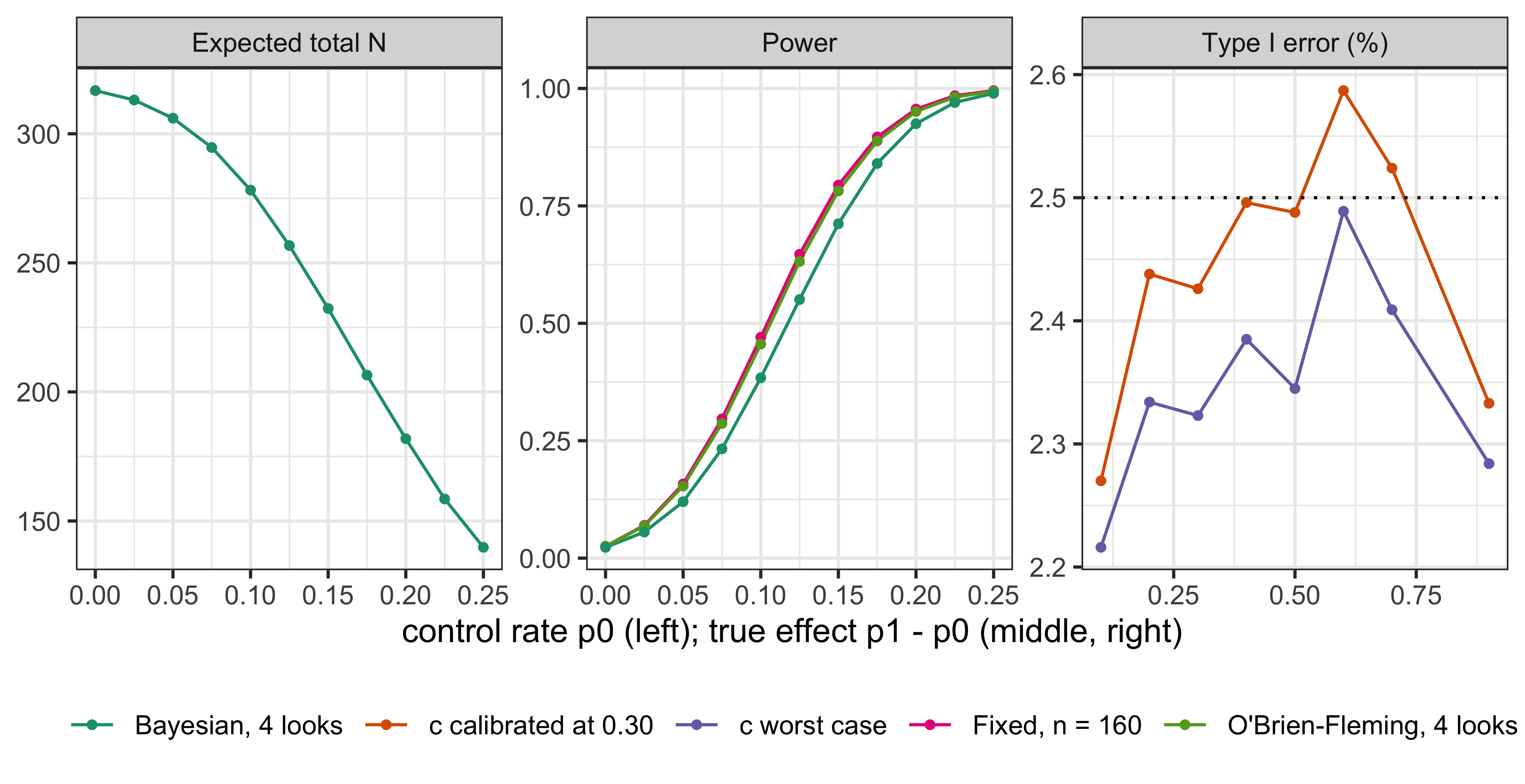
The three panels of Figure 14.1 show the null grid, the power curves and the expected sample size.
Show the R code
ds <-seq(0, 0.25, length.out =11)bay <-lapply(ds, function(d) oc_summarize(oc_simulate(0.3, 0.3+ d, looks, nsim =2e4, seed =7), c0))dr <-function(d) d /sqrt(2* (0.3+ d /2) * (0.7- d /2) /160)L <-rbind(data.frame(panel ="Type I error (%)", x = grid, y = null_tab$error, design ="c calibrated at 0.30"),data.frame(panel ="Type I error (%)", x = grid, y =sapply(nulls, function(s) 100*oc_summarize(s, c_wc)$reject), design ="c worst case"),data.frame(panel ="Power", x = ds, y =sapply(ds, function(d) exact(0.3, 0.3+ d)), design ="Fixed, n = 160"),data.frame(panel ="Power", x = ds, y =sapply(ds, function(d) gs_power(tt, bound, drift =dr(d))), design ="O'Brien-Fleming, 4 looks"),data.frame(panel ="Power", x = ds, y =sapply(bay, `[[`, "reject"), design ="Bayesian, 4 looks"),data.frame(panel ="Expected total N", x = ds, y =sapply(bay, `[[`, "EN"), design ="Bayesian, 4 looks"))L$panel <-factor(L$panel, c("Type I error (%)", "Power", "Expected total N"))ggplot(L, aes(x, y, colour = design)) +geom_line() +geom_point(size =1) +facet_wrap(~panel, scales ="free") +geom_hline(data =data.frame(panel ="Type I error (%)", y =2.5), aes(yintercept = y), linetype =3, inherit.aes =FALSE) +scale_colour_brewer(palette ="Dark2") +labs(x ="control rate p0 (left); true effect p1 - p0 (middle, right)", y =NULL, colour =NULL) +theme_bw() +theme(legend.position ="bottom")
Figure 14.1: Left: type I error across control rates, with the threshold calibrated at p0 = 0.30 and with the worst-case threshold; dotted line at 2.5 percent. Middle: power of the fixed design, the O’Brien-Fleming design (analytic) and the four-look Bayesian design (simulated) against the true effect. Right: expected total sample size of the Bayesian design.
The worst-case threshold moves \(c\) by only \(0.0003\), so its effect on power is negligible, and it pulls the null curve down toward the line. In the middle panel the Bayesian design has power 0.713 at an effect of 0.15, below the fixed design’s 0.794 and the O’Brien-Fleming design’s 0.782; the right panel shows the expected sample size, which falls from 317 at the null to 140 at an effect of 0.25. In this example the Bayesian design is a group sequential design with a particular boundary: nothing about the posterior probability makes it more efficient than a well-chosen frequentist boundary, and the benefits that come from Bayesian adaptive designs in later chapters (borrowing, predictive stopping, dose selection, response-adaptive allocation) come from structure that a group sequential design does not have. The agreement of the single-look case with the exact enumeration is itself a check on the code (Section 14.9).
14.6 Scenario grids, the worst case, and what the grid must span
A simulation study is a set of scenarios, and the scenarios decide whether the report convinces. The FDA’s 2019 guidance asks for a range of plausible parameter values, including the null space; the Bayesian draft asks that the operating characteristics be shown across the effect sizes of interest, and, for designs that are not calibrated to type I error, that the probability of a positive conclusion be reported over the range (U.S. Food and Drug Administration 2019, 2026). The following structure covers what reviewers usually need.
Efficacy scenarios. The global null; the design alternative; an intermediate alternative (half of the design effect is the convention); a small-effect alternative close to the minimum clinically relevant effect \(a\); and a large effect. For multi-arm designs add: one effective arm among several, a monotone dose response, a peaked dose response, and several near-maximal arms. A table of power and the probability of incorrect selection (choosing a wrong arm) by scenario is the standard report.
Nuisance scenarios. For a binary endpoint, the control rate (as in the null grid above); for a continuous endpoint, the standard deviation; for time-to-event, the control hazard and accrual pattern. These are the parameters that the type I error must be robust to, and where the “worst case null” is found: the supremum of the error over the nuisance space under the null. A grid is a pragmatic search, and one reports the grid spacing and where the maximum fell. If the maximum falls at the edge of the grid, the grid was too small.
Operational scenarios. Accrual rate (slow, expected, fast), dropout, outcome delay, site activation, and, for platform trials, arm arrival. A phase 2 platform screening design with fixed-size arms and a limit on concurrent arms can fail in this way: a single effective arm that arrives late may never be started, a failure of operations and not of statistics, visible only in a simulation that models arrivals. Operational assumptions can dominate the efficacy assumptions.
Misspecification scenarios. Time trends in the control rate (when non-concurrent controls are used), prior-data conflict (when a prior from external data is used), non-proportional hazards, and heterogeneity. The point of these is to show how the operating characteristics degrade when the model is wrong, and what the monitoring plan does about it. The draft guidance’s emphasis on a prespecified prior and on the effect of the prior on the operating characteristics is, in simulation terms, a request for a prior-conflict scenario grid (Chapter 8).
Sampled-effect scenarios. When the sponsor has a prior over effects, as in a portfolio or a phase 2 program, the true effect may be sampled from it, and the report gives probabilities by the true class of the effect (null, mediocre, good) in addition to the overall rates. This gives the assurance-style number (the probability of success averaged over the prior, Chapter 9), but the report must also give the rates conditional on the true state, because the type I error is a statement about the null only.
For each of these, the design is fixed first, then run across all scenarios without modification. Tuning a design to make the scenario table look good and then reporting the table is legitimate, if the final design is then frozen and revalidated on fresh seeds; the report should say that the tuning happened and which scenarios drove it. The “worst case” of the type I error is not itself a probability under a model: it is the maximum over a set of models the sponsor decides to consider, and the report should state what set that is.
14.7 The Goldilocks design
The industrial practice of Bayesian adaptive design (associated with Berry Consultants and the simulator FACTS) has one organizing principle: the design is chosen by simulation rather than derived in closed form. It describes its own method as flight-simulating a trial: a structure is specified, many assumed truths are simulated, and the design is judged by how it behaves across all of them (Polson and Sokolov 2026; S. M. Berry et al. 2010). The operating characteristics reported are power, type I error, expected sample size, expected duration, assurance and the probability of correct selection. The published comparison with conventional packages is explicit about the division of labor: those packages are built for analytic type I error control and closed-form sample size, while the simulator is built for structures that have no closed form, with conventional group sequential and promising-zone designs available as special cases.
The idea is older than the industry, and its history explains why a Bayesian design is judged by frequentist operating characteristics. Lewis and Berry’s classical evaluation of Bayesian decision-theoretic designs (Lewis and Berry 1994) illustrates the operating-characteristic perspective used here; Section 1.9 and Section 15.6 give the historical development and backward-induction construction. Thall and Simon (1994) chose Bayesian phase 2 stopping rules by their frequentist operating characteristics. Müller et al. (2007) formalized simulation-based sequential Bayesian design, the approach of the adaptive dose-ranging designs of D. A. Berry et al. (2002). The principle that a Bayesian procedure should be calibrated to long-run frequency behavior is stated by Rubin (1984), Spiegelhalter, Freedman, and Parmar (1994) and Little (2006), and the calibration of this chapter is that principle applied to a posterior threshold.
The signature construction is the Goldilocks sample size design of Broglio, Connor and Berry (Broglio, Connor, and Berry 2014): a trial that does not fix its sample size but lets accrual run until the data say the sample is “not too big, not too small.” At each look it computes two predictive probabilities, \(\mathrm{PP}_{\text{stop}}\) (success if enrollment stops now and the pending outcomes are completed) and \(\mathrm{PP}_{\max}\) (success at the maximum sample size). It stops enrolling for expected success when the first is high and stops for futility when the second is low; the construction and a worked example are in Section 15.5. The full design of Broglio and colleagues also has an immediate-success rule, a higher threshold on \(\mathrm{PP}_{\text{stop}}\) at which success is declared without following the pending patients; it is not used here, where outcomes are immediate. The sample size is an output, bounded by \(N_{\max}\), not a design input, and the thresholds are calibrated by simulating type I error, not derived. Where this construction sits among the calibration devices, relative to the spending boundary and the moderate-deviation boundary of the working paper, is an open question there: the working paper conjectures a moderate-deviation rule with a data-dependent constant, and does not claim a proof. Predictive probabilities, the choice of thresholds, and the delayed-outcome model are developed in Chapter 15.
For a trial with immediate outcomes, as in the example, \(\mathrm{PP}_{\text{stop}}\) collapses to an indicator of whether the posterior rule is already met, and what is left of Goldilocks is the futility rule based on \(\mathrm{PP}_{\max}\). The chunk below uses the exact beta-binomial predictive probability of the posterior rule being met at 160 per arm, stops for futility if it falls below \(F = 0.05\) at any of the first three looks, and recalibrates \(c\) by iteration, because \(c\) appears both in the success rule and inside the predictive probability.
Table 14.7: Goldilocks-style futility (stop if the predictive probability of success at 160 per arm is below 0.05) against efficacy-only stopping, four looks, flat priors, c recalibrated to 2.5 percent. 40,000 trials per row for the null and 40,000 per alternative (SE at most 0.0025).
Effect
Power, efficacy only
E[N]
Power, with P_max futility
E[N]
P(futility stop)
0.00
0.026
316
0.026
150
0.902
0.05
0.124
305
0.121
189
0.691
0.10
0.384
277
0.371
213
0.401
0.15
0.715
232
0.694
206
0.164
0.20
0.926
182
0.911
173
0.047
Under the null the predictive futility rule stops \(90\) percent of trials before the end and cuts the expected sample size from \(316\) to \(150\), more than half. It does this at a price in power of up to \(2.2\) percentage points, largest at the design alternative \(0.15\) (\(0.715\) falls to \(0.694\)), where a trial with a true moderate benefit has a real chance of looking hopeless at 40 or 80 per arm. That price is the cost of the futility rule, and the table shows it. A sponsor who chooses \(F\) by looking at this table is choosing a point on the frontier between expected sample size under the null and power against modest effects, which is the decision that the Goldilocks name refers to.
The Goldilocks sketch above omits the part that needs a delayed-outcome model (the stop-accrual rule and the completion of follow-up), and the design in a real FACTS project would add arms, longitudinal models for early outcomes, and a different success rule. DAWN’s analysis plan is a trial-sized version of this construction, with predictive-probability stopping thresholds that fall with sample size and a success threshold that rises when the population is enriched (Section 14.11).
The same practice has built platform trials: I-SPY 2, a breast cancer platform enrolling since 2010 that shares controls, drops arms early for futility or efficacy, reinvests freed resources in new agents and uses longitudinal imaging to predict its pathologic response endpoint; GBM AGILE, a glioblastoma platform; and the critical care and pandemic platforms including REMAP-CAP and the ACTIV family. Basket designs include a nine-cancer study of a combination in rare mutation-defined tumors whose primary analysis borrows across the nine groups, and which supported a pan-tumor approval in 2022 (Polson and Sokolov 2026). These are the trials in which simulation is the only available route, and they are the subject of Chapter 20 and Chapter 19 (the I-SPY 2 and GBM AGILE decision rules are in Section 15.10). One caution in the same source: the public material contains no measured efficiency claims. The benefits asserted (smaller samples, fewer patients on placebo, lower cost and shorter timelines) have no quantity attached to them, which is why the numbers in this chapter are computed, not quoted.
14.8 What the simulation report must contain
The FDA’s adaptive designs guidance, the Bayesian draft and ICH E20 differ in detail and agree in substance. Section VI of the 2019 guidance treats simulation as the way to estimate the operating characteristics of designs that have no analytic solution and says what a submission should document: the simulation plan, the software or code, the number of replicates and the results, across a range of plausible values that includes the null space (U.S. Food and Drug Administration 2019). The Bayesian draft separates designs calibrated to type I error control (for which the key characteristic is the type I error, controlled at a given level, typically 0.025 one-sided) from designs that are not (where the sponsor reports the probability of a positive conclusion across effect sizes, along with the bias and variability of the estimates), and asks for extensive documentation of simulations, code and software, and for the effect of the prior on the operating characteristics (U.S. Food and Drug Administration 2026). ICH E20 defines a simulation as “the repeated execution of a large number of hypothetical clinical trials” in Section 5.2 and, in Section 5.3, says that Bayesian adaptive designs must show targeted operating characteristics and maintain type I error control (International Council for Harmonisation 2025). The three documents are drafts or guidance, not law, and a sponsor can propose another approach; but a submission that omits what they list is unlikely to survive review without a good reason.
A structure that satisfies all three is the ADEMP framework of Morris, White and Crowther: aims, data-generating mechanisms, estimands, methods and performance measures (Morris, White, and Crowther 2019). Table 14.8 maps the elements of a simulation report to it and to the source of each requirement.
Table 14.8: Contents of a simulation report.
Element
What the report states
Where it comes from
Aims
The decisions the design supports; the target operating characteristics (\(\alpha\), power, maximum \(N\))
FDA 2019 Section III; E20 Section 5.2
Design as simulated
Every rule: priors, success criterion \((a, c)\), looks (by information, events or calendar), futility, allocation, selection; binding or non-binding futility
FDA Bayesian IV.A; E20 Section 5.2
Calibration
How \(c\) (and \(a\)) were chosen; the null scenario used; the worst-case search over nuisance parameters; the grid
FDA Bayesian IV.A.1
Scenarios
All data-generating parameters of each scenario, and why chosen; null space, misspecification, operational
FDA 2019 Section VI.A
Estimand
The primary estimand per hypothesis and how intercurrent events are simulated
ICH E9(R1)
Performance measures
Type I error (per hypothesis and familywise); power by scenario; expected and maximum \(N\) (enrolled, not only completers); probability of stopping at each look and why; bias, variability, coverage of the estimates at stopping
FDA 2019 Section III; FDA Bayesian
Monte Carlo error
Number of replicates and the standard error of every reported rate
FDA 2019 Section VI
Prior
The prior, its justification and a sensitivity analysis of the operating characteristics to it
FDA Bayesian draft, Section V
Software and reproducibility
Program, version, random number generator, seeds, MCMC settings if any, the code itself
FDA 2019 Section VI; FDA Bayesian
Example trials
A handful of individual simulated trials plotted, so that a reader can see how the rules behave
Practice (Berry Consultants), E20
Traceability
The simulated design is the protocol and SAP design, line by line, with a change log
E20 Section 5.2
Three items in this table are where reports most often fall short. The first is the enrolled-versus-completed distinction. A trial with a 24-week endpoint that stops when 80 patients have completed has probably enrolled more: the analytic expected sample size of a group sequential design counts completers, while a simulation that models accrual counts everyone enrolled, which is larger because patients still in the pipeline count when the trial stops. The second is binding and non-binding futility: if the data monitoring committee can ignore a futility recommendation, the type I error must be calibrated with the futility rule ignored. The third is traceability: the code that was simulated and the rules in the protocol must be the same rules, and the easiest way to ensure this is to generate both from one specification.
Two practice sources complement the regulatory documents. Mayer et al. (2019) survey simulation practices for adaptive designs in drug and device development, the practitioner counterpart of Table 14.8. And when the trial itself is reported, the CONSORT extension for adaptive designs (ACE) of Dimairo et al. (2020) is the checklist that journals ask for: its items on the pre-specified adaptations and on how they can affect the estimates correspond to the rows “Design as simulated” and “Performance measures” above, so the simulation report supports ACE reporting of design properties and estimation methods. ACE additionally calls for reporting the adaptations actually made, departures from planned rules, participant flow and arrangements protecting trial integrity.
TipIn the protocol: language for the simulation section
[Template: bracketed values, Table X and Appendix Y are placeholders to be completed by the sponsor.] “The success criterion is \(\Pr(p_1 - p_0 > 0 \mid \text{data}) > c\) at any of four looks (40, 80, 120 and 160 patients per arm), with independent Beta(1,1) priors. The threshold \(c\) was calibrated by simulation so that the familywise one-sided type I error rate is at most 0.025 across a grid of control rates (0.1 to 0.7 in steps of 0.1, and 0.9) and under all null hypotheses \(p_1 \le p_0\), using \(10^5\) simulated trials per scenario; the resulting \(c\) is [value], and the type I error was verified on an independent run of \(4 \times 10^5\) trials with a different seed (maximum observed error [value], Monte Carlo SE 0.00025). Operating characteristics for the scenarios in Table X are in the simulation report (version, date, SHA of the code), which is part of this protocol. The simulation code, random seeds and software versions are provided in Appendix Y.”
14.9 Software, reproducibility and what to submit
Four kinds of software appear in submissions. Commercial design packages include FACTS (Berry Consultants), which has core engines for continuous, dichotomous and time-to-event endpoints, dose-finding and staged designs, and a platform-trial engine, and East (Cytel), the industry standard for group sequential and frequentist adaptive designs. Analytic open-source packages such as rpact and gsDesign in R compute group sequential boundaries, power and sample size reassessment without simulation, and are the right tool for the traditional half of a design (Wassmer and Brannath 2016; Jennison and Turnbull 2000). Open-source simulation packages for Bayesian adaptive designs exist in R (adaptr, and the bayestrials package used in this book, for example) and are validated by their users. Custom code in R, Python or Stan is needed for bespoke platforms or borrowing, and with custom code the sponsor owns the verification. The regulator asks for the code.
Whichever is used, verification is the sponsor’s job, and there are three cheap tests. Reproduce a known analytic result: with one look and \(c = 0.975\) the simulator’s type I error should be close to the exact enumeration of the fixed design (0.0252 above; the check below gives a little under that, because the Bayesian rule and the pooled \(z\) test differ slightly at discrete counts), and a Bayesian rule with a boundary borrowed from a group sequential design should reproduce the analytic rejection probability, so the code is checked at the points where the answer is known. Check invariances: the type I error should not depend on the label of the arms, and a design with \(K = 1\) should be the fixed design. Run the simulation twice with different seeds and compare: the difference should be of the size of the Monte Carlo error. Never leave debug settings in a final run (one burn-in sample to speed up a Markov chain Monte Carlo fit makes every Bayesian output meaningless while the frequentist outputs look fine).
Show the R code
one <-oc_simulate(0.3, 0.3, 160, nsim =4e5, seed =3) # K = 1 must reproduce the fixed designw1 <-unlist(oc_summarize(one, 0.975))[c("reject", "se_reject")]knitr::kable(data.frame(Quantity =c("Type I error", "Monte Carlo SE"), Value =round(unname(w1), 5)))
Quantity
Value
Type I error
0.02456
Monte Carlo SE
0.00024
Reproducibility means fixing the random number generator and the seed, recording the software and package versions, and archiving the code and outputs with the report. In this book every simulation passes seed = to oc_simulate, which sets the generator before drawing. Parallel runs should use independent streams, for example L’Ecuyer-CMRG streams from parallel::nextRNGStream, not the same seed on every worker. A one-line record of the environment goes in the report:
The final run that supports the submission should be a clean execution of the frozen code from a frozen specification, not the last of a sequence of exploratory edits.
In submitting, the FDA’s Complex Innovative Trial Design paired meeting program (Chapter 3) expects a simulation report ahead of the meeting; the report is then the object under discussion, and the agency’s comments are on its scenarios and calibration. The practice for a late-phase confirmatory trial is the same: send the simulation plan before the trial starts, send the code if asked, and expect questions about the null space and the prior (Chapter 23). A simulation done after the data are in is not a prespecified operating characteristic, however carefully it is done.
14.10 Traditional and Bayesian side by side
Traditional (fixed or group sequential)
Bayesian adaptive, calibrated
Decision rule
\(Z_k > b_k\) at look \(k\)
\(\Pr(\delta > a \mid \text{data}) > c\) at look \(k\)
Type I error
Computed analytically from the joint normal distribution of the \(Z_k\)
Computed by simulation; \(c\) (and \(a\)) chosen so that it is 0.025 one-sided
Power and expected \(N\)
Analytic for stated alternatives
Simulated across a scenario grid
What the SAP states
Sample size, boundaries or spending function, test
The above, plus the prior, the calibration and the simulation report
What changes under complexity
Closed form fails; simulation is added
Simulation is usually the method (exact recursion for some rules)
Agreement
With a flat prior and a normal likelihood the posterior probability of benefit is \(1 - p\) for the one-sided \(p\)-value at a single look
The same, for a single look; calibration targets the overall probability of any false efficacy conclusion across the looks, and the distribution of that error across looks need not match the traditional design
What the regulator asks
Is the boundary prespecified and the multiplicity handled?
Is the simulation complete, reproducible, and is the null space covered?
Where the traditional design is the better choice, it is for reasons that this chapter makes concrete. When the design is a single look or a standard group sequential design with a known boundary, the analytic computation is exact, cheaper to verify and carries no Monte Carlo error: a reviewer can reproduce it in a minute. A sponsor that cannot commit to the prespecification and the code that a simulation-based design requires should not choose one.
14.11 In practice
Four submissions show what a calibrated posterior threshold looks like in a protocol, a statistical analysis plan or a device summary.
BNT162b2: thresholds chosen for a 2.5 percent overall error
The pivotal phase 2/3 trial of the Pfizer and BioNTech vaccine (protocol C4591001) is described, with its model and clinical result, in Section 21.5, and its posterior computation in Chapter 6. For this chapter only the calibration matters. The analysis plan on ClinicalTrials.gov sets the posterior threshold at 0.995 at an interim analysis and 0.986 at the final analysis (164 first primary cases), chosen so that the overall one-sided type I error is 2.5 percent (Pfizer Inc. 2022). The futility rule of the plan is described in Section 15.10. The lesson for this chapter is the shape of the calibrated rule: a single posterior probability does not control the error across looks, so the threshold is stricter at the interim looks, which spend little of the error, than at the final analysis (0.995 early, 0.986 at the end). The plan posted on ClinicalTrials.gov is one of several amended versions.
REBYOTA: two thresholds, adjusted for the information fraction
The phase 3 trial of RBX2660 for recurrent C. difficile infection (the full case is in Section 19.17.1) chose two posterior thresholds as analogues of one-sided type I error rates of 0.00125 and 0.025 without borrowing, and at study end adjusted them for the information fraction actually reached (0.9993275 and 0.9750338) (U.S. Food and Drug Administration, Center for Biologics Evaluation and Research 2022). The result, a posterior probability of superiority of 0.991, met the second threshold but not the first. The lesson is the one the Lan-DeMets method teaches for \(z\) boundaries: a threshold calibrated for a planned information fraction is recomputed for the realized one, and the rule for doing so belongs in the plan before the data. A posterior of 0.991 is also close to the \(c = 0.9907\) of this chapter’s example, which 0.991 only just clears: a result well above the single-look 0.975 can sit at the edge of a calibrated multi-look bar.
DAWN: a success threshold that moves with the enrichment
The DAWN trial of thrombectomy 6 to 24 hours after stroke used a Bayesian adaptive enrichment design. Its analysis plan takes a baseline success threshold of 0.986 on the posterior probability of superiority, chosen by simulation to control the type I error, and raises it if enrichment occurs: the threshold is \(\Phi\bigl(\sqrt{1 + N_2/(N_1 + N_3)}\;\Phi^{-1}(0.986)\bigr)\), where \(N_1\) patients are in the enriched population at the decision, \(N_2\) outside it and \(N_3\) enrolled after it (Stryker Neurovascular 2017). As an illustration, if the patients outside the enriched population were half of the rest the threshold would be \(0.9964\). The predictive-probability stopping schedule of the plan is in Section 15.10. The trial stopped at the first efficacy look with 206 patients and 49 percent against 13 percent functional independence (Nogueira et al. 2018). The lesson is that calibration extends to adaptations: every branch of the design (enrich or not, stop or not) needs its threshold computed so that the error is controlled on all of them.
Superion: a device threshold of 0.958
The Superion interspinous spacer trial (PMA P140004) randomized against a comparator device with a Bayesian adaptive sample size of 250 to 350 evaluable patients, a non-inferiority margin of 10 percent, flat Beta(1,1) priors and success if the posterior probability of non-inferiority was at least 0.958, a value chosen to control the type I error below 0.05; the stated power was 86.3 percent (U.S. Food and Drug Administration, CDRH 2015). The final modified intention-to-treat sample was 190 against 201 patients, and the posterior probability of non-inferiority was 0.9927 (0.9944 per protocol), above the threshold, with approval on 20 May 2015. The lesson is that 0.958 is not a conventional number: it is what a simulation of this particular margin, prior, error budget and adaptive sample size returned, and the device summary reports it as such. The practice of calibrating a Bayesian threshold to a frequentist error rate by simulation is described in the FDA’s 2010 guidance on Bayesian statistics in medical device clinical trials (U.S. Food and Drug Administration 2010), and in the accounts of reviewers who handled such submissions (Pennello and Thompson 2008; Campbell 2011).
TipTry it in the lab
Open the adaptive Bayesian module at https://nytel.ai/testing/09-adaptive-bayesian.html. Before moving the “Bar” slider, predict what happens to the false-positive rate when the trial is allowed to stop at any interim look at the same posterior threshold, then check. Then open the Bayesian trial simulator, module 14, at https://nytel.ai/testing/14-simulator.html: set the null, vary the number of looks and the threshold, and find the threshold that holds the false-positive rate at 2.5 percent, as in Table 14.1. Its group sequential comparison uses Lan-DeMets O’Brien-Fleming-type spending by default (4.333, 2.963, 2.359, 2.014), with the classical boundaries (4.049, 2.863, 2.337, 2.024) as a toggle. The full open simulator is at https://nytel.ai/testing/14-studio.html.
Key points
A traditional SAP states analytic operating characteristics: the type I error follows from the sampling distribution of the test statistic, and power is computed at stated alternatives. Complex adaptations often require simulation, although some posterior and predictive stopping rules permit analytic calculation or exact recursive enumeration (FDA 2019 Section VI.A describes simulation as a major use).
The Bayesian success rule \(\Pr(\delta > a \mid \text{data}) > c\) has no type I error until the whole procedure (priors, looks, \(a\), \(c\)) is fixed. At \(c = 0.975\) with four looks the error in the example is 6.3 percent, and with 32 looks 12.8 percent; the working paper behind this book reports 12.0 percent for continuous monitoring in a SELECT-based setting.
Calibration chooses \(c\) (given \(a\)) as the \((1-\alpha)\) quantile of the maximum posterior probability under the null. In the example \(c = 0.9907\) gives 2.5 percent for four looks, and the worst case over control rates needs about \(0.991\). Real plans state such calibrated thresholds: 0.995 and 0.986 for BNT162b2, 0.9993275 and 0.9750338 for REBYOTA, 0.958 for Superion.
The type I error must hold over the null space, not at one point: report a grid over the nuisance parameters, the location of the maximum, and the boundary \(p_1 < p_0\).
Report power, expected sample size, probability of stopping early, and the bias at stopping. In the example the four-look design stops early for success 57 percent of the time at the design alternative, saves about 28 percent of the sample, loses about 8 points of power against the fixed design, and overstates the effect by about 0.08 among the trials that stop early.
Monte Carlo error is binomial: 0.0016 at 10,000 trials for a rate of 0.025, 0.0005 at 100,000. Calibrate on at least \(10^5\) trials, and validate on a fresh seed.
The Goldilocks design lets the sample size be an output, bounded by \(N_{\max}\), governed by predictive probabilities of success; its thresholds are calibrated by simulation, not derived.
A simulation report states aims, scenarios, every rule, the calibration, performance measures with Monte Carlo errors, the prior sensitivity, software, seeds and code, and it must match the protocol line by line (FDA Bayesian draft IV.A.1; FDA 2019 Section VI; ICH E20 Sections 5.2 and 5.3).
NoteDiscussion questions
The calibrated threshold for four looks is \(c = 0.9907\), which is more demanding than the 0.975 of a one-sided test. A sponsor argues that this makes the Bayesian design “less efficient” than a fixed trial. Using the table of operating characteristics, say what the design buys in return, and under which scenarios it does not pay for itself.
A reviewer finds that the type I error is 2.59 percent at a control rate of 0.60, though the design was calibrated at 0.30. Is this a violation, a Monte Carlo artifact, or both? What would you do to decide, and how many simulated trials would you need?
Choose between \((a, c) = (0, 0.9907)\) and \((0.10, 0.849)\), both of which give 2.5 percent type I error. What clinical and regulatory arguments favor each, and what does the second pair do to power at small effects?
The estimate at stopping is biased upwards among trials that stop early for success. Should the protocol report the naive estimate, a bias-adjusted estimate, or both? What would a regulator accept?
A platform design has no closed-form operating characteristics. List five scenarios you would insist on seeing in the simulation report, including at least one operational and one misspecification scenario.
Berry, Donald A., Peter Müller, Andrew P. Grieve, Michael Smith, Thomas Parke, Robert Blazek, Neil Mitchard, and Martin Krams. 2002. “Adaptive Bayesian Designs for Dose-Ranging Drug Trials.” In Case Studies in Bayesian Statistics v, 162:99–181. Lecture Notes in Statistics. New York: Springer.
Berry, Scott M., Bradley P. Carlin, J. Jack Lee, and Peter Müller. 2010. Bayesian Adaptive Methods for Clinical Trials. Boca Raton: CRC Press.
Broglio, Kristine R., Jason T. Connor, and Scott M. Berry. 2014. “Not Too Big, Not Too Small: A Goldilocks Approach to Sample Size Selection.”Journal of Biopharmaceutical Statistics 24 (3): 685–705. https://doi.org/10.1080/10543406.2014.888569.
Campbell, Gregory. 2011. “Bayesian Statistics in Medical Devices: Innovation Sparked by the FDA.”Journal of Biopharmaceutical Statistics 21 (5): 871–87. https://doi.org/10.1080/10543406.2011.589638.
Dimairo, Munyaradzi, Philip Pallmann, James Wason, Susan Todd, Thomas Jaki, Steven A Julious, Adrian P Mander, et al. 2020. “The Adaptive designs CONSORT Extension (ACE) statement: a checklist with explanation and elaboration guideline for reporting randomised trials that use an adaptive design.”BMJ, m115. https://doi.org/10.1136/bmj.m115.
Jennison, Christopher, and Bruce W. Turnbull. 2000. Group Sequential Methods with Applications to Clinical Trials. Boca Raton, FL: Chapman & Hall/CRC.
Lewis, Roger J., and Donald A. Berry. 1994. “Group Sequential Clinical Trials: A Classical Evaluation of Bayesian Decision-Theoretic Designs.”Journal of the American Statistical Association 89 (428): 1528–34. https://doi.org/10.1080/01621459.1994.10476893.
Mayer, Cristiana, Inna Perevozskaya, Sergei Leonov, Vladimir Dragalin, et al. 2019. “Simulation Practices for Adaptive Trial Designs in Drug and Device Development.”Statistics in Biopharmaceutical Research 11 (4): 325–35. https://doi.org/10.1080/19466315.2018.1560359.
Morris, Tim P., Ian R. White, and Michael J. Crowther. 2019. “Using simulation studies to evaluate statistical methods.”Statistics in Medicine 38 (11): 2074–2102. https://doi.org/10.1002/sim.8086.
Müller, Peter, Donald A. Berry, Andrew P. Grieve, Michael Smith, and Michael Krams. 2007. “Simulation-Based Sequential Bayesian Design.”Journal of Statistical Planning and Inference 137 (10): 3140–50. https://doi.org/10.1016/j.jspi.2006.05.021.
Nogueira, Raul G., Ashutosh P. Jadhav, Diogo C. Haussen, Alain Bonafe, Ronald F. Budzik, Parita Bhuva, Dileep R. Yavagal, et al. 2018. “Thrombectomy 6 to 24 Hours after Stroke with a Mismatch between Deficit and Infarct.”New England Journal of Medicine 378 (1): 11–21. https://doi.org/10.1056/NEJMoa1706442.
O’Brien, Peter C., and Thomas R. Fleming. 1979. “A Multiple Testing Procedure for Clinical Trials.”Biometrics 35 (3): 549–56.
Pennello, Gene, and Laura Thompson. 2008. “Experience with Reviewing Bayesian Medical Device Trials.”Journal of Biopharmaceutical Statistics 18 (1): 81–115. https://doi.org/10.1080/10543400701668274.
Polson, Nicholas G., and Vadim Sokolov. 2026. “Bayesian Versus Standard Clinical Trial Design: Theory, Evidence, and Protocol.”
Rubin, Donald B. 1984. “Bayesianly Justifiable and Relevant Frequency Calculations for the Applied Statistician.”The Annals of Statistics 12 (4): 1151–72. https://doi.org/10.1214/aos/1176346785.
Spiegelhalter, David J., Laurence S. Freedman, and Mahesh K. B. Parmar. 1994. “Bayesian Approaches to Randomized Trials.”Journal of the Royal Statistical Society, Series A 157 (3): 357–416. https://doi.org/10.2307/2983527.
Thall, Peter F., and Richard Simon. 1994. “Practical Bayesian Guidelines for Phase IIB Clinical Trials.”Biometrics 50 (2): 337–49. https://doi.org/10.2307/2533377.
U.S. Food and Drug Administration. 2010. “Guidance for the Use of Bayesian Statistics in Medical Device Clinical Trials.”U.S. Food and Drug Administration. https://www.fda.gov/media/71512/download.
U.S. Food and Drug Administration, Center for Biologics Evaluation and Research. 2022. “FDA Briefing Document, Vaccines and Related Biological Products Advisory Committee Meeting, September 22, 2022: RBX2660 (Fecal Microbiota Suspension for Rectal Enema), Rebiotix, Inc., BLASTN 125739.”https://www.fda.gov/media/161679/download.
Wassmer, Gernot, and Werner Brannath. 2016. Group Sequential and Confirmatory Adaptive Designs in Clinical Trials. Springer. https://doi.org/10.1007/978-3-319-32562-0.