15Predictive Probability, Interim Monitoring, and Stopping
Every interim look asks the same question in different words: given what we have seen, what will happen if we carry on? A data monitoring committee (DMC) that sees a borderline interim result wants to know whether the trial can still succeed, how many more patients it would take, and whether the money and the patients’ time are better spent elsewhere. The traditional trial answers with conditional power, a number computed from the interim data and an assumed effect. The Bayesian trial answers with the predictive probability of success, the same calculation averaged over what the data say about the effect. This chapter builds both, shows that they are close relatives, and then follows the idea to its logical end: a stopping rule that is optimal for a stated loss, found by working backward from the end of the trial.
The chapter uses three tools that appear in the earlier chapters. The beta-binomial posterior is from Chapter 6. The group sequential boundaries and the error-spending logic are from Chapter 11. The simulation report that every design must carry is from Chapter 14.
ImportantRegulatory anchor
The documents below govern interim monitoring and stopping. Chapter 3 describes each one in full and gives its status.
ICH E9, Statistical Principles for Clinical Trials (1998), section 4.5, interim analysis and early stopping. Defines an interim analysis as “any analysis intended to compare treatment arms with respect to efficacy or safety at any time prior to formal completion of a trial”, and requires that “all interim analyses should be carefully planned in advance and described in the protocol” (PDF p23). The statistical methods “should be fully specified in advance of the availability of information on treatment outcomes” (section 3.4, PDF p20).
FDA, Adaptive Designs for Clinical Trials of Drugs and Biologics (final guidance, November 2019). Treats sample size adaptation and futility stopping as adaptations that must be prospectively planned, with type I error control and bias addressed. Notes that adaptive features “can inflate the Type I error probability of a trial” (section III.A, PDF p11), and asks that interim results be walled off from those running the trial (sections III and VII).
ICH E20, Adaptive Designs for Clinical Trials (Step 2 draft, June 2025). Recommends that adaptations be “pre-specified in the clinical trial protocol prior to initiation of the trial” (section 1, PDF p6), warns that “the Type I error probability can be more than doubled” under analysis methods that ignore the adaptation (section 2, PDF p7), and expects simulation of operating characteristics such as “power, expected sample size, reliability of adaptation decisions” (section 2, PDF p8). Section 5.3 says a Bayesian adaptive design must still show targeted operating characteristics “while maintaining Type I error probability control” (PDF p29). A draft, not binding.
FDA, Use of Bayesian Methodology in Clinical Trials of Drug and Biological Products (draft guidance, January 2026). The success criterion is of the form \(\Pr(\delta > a \mid \text{data}) > c\), and, for trials with an overall frequentist statistical analysis plan, familywise type I error is “almost always” held at 0.025 one-sided (section IV.A, PDF p10). The draft also describes direct interpretation of posterior probabilities and decision-theoretic criteria (section IV.A.3), and calibration to error control is this book’s default, not the only route. In this book’s reading (not the draft’s wording), a predictive probability rule is a design component of the same kind: it is acceptable to the extent that its simulated operating characteristics are reported and its thresholds are fixed before the trial. A draft, not binding.
15.1 The traditional interim: conditional power and futility
Conditional power
A trial is designed for a fixed sample size with one-sided \(\alpha = 0.025\) and power \(1-\beta\) at a design alternative \(\xi_a\) (Chapter 9). Partway through, at information fraction \(t\) (the share of planned patients or events observed), the DMC has a standardized statistic \(Z_t\). The question “could this trial still win?” has a precise form. Conditional power is the probability that the final statistic \(Z_1\) exceeds the critical value \(z_\alpha\), given the interim data and an assumed value of the effect.
The calculation uses the independent-increments structure of the test statistic. Write the B-value(Lan and Wittes 1988)\(B_t = Z_t\sqrt{t}\), the cumulative sum of the standardized information. Let \(\xi\) denote the drift, the expected value of the final \(Z_1\), so that under the design alternative \(\xi = z_\alpha + z_\beta\). The symbol \(\theta\) is reserved for the treatment effect; \(\xi = \theta\sqrt{I_{\max}}\) is its standardized final drift. Then the future increment \(B_1 - B_t\) is normal with mean \(\xi(1-t)\) and variance \(1-t\), whatever the past was, and
Everything depends on the choice of \(\xi\), and three choices are in use. Under the design alternative, \(\xi = z_\alpha + z_\beta\): this asks whether the trial can still succeed if the sponsor’s original belief was right. Under the current trend, \(\xi = Z_t/\sqrt{t}\): this asks what happens if the effect seen so far is the true effect. Under the null, \(\xi = 0\): this asks whether the trial can win by luck alone. The first is optimistic after a poor interim, the second is pessimistic after a poor interim and optimistic after a good one, and the third is the floor.
Conditional power is the basis of stochastic curtailment, introduced for clinical trials by Lan, Simon, and Halperin (1982), with the companion conditional-power monitoring tool of Halperin et al. (1982): stop when the outcome is nearly decided one way or the other. Proschan, Lan, and Wittes (2006) give the modern treatment.
Table 15.1: Conditional power at half the information (t = 0.5) of a trial designed with 90 percent power at one-sided 0.025 (design drift 3.24), under the design alternative, the current trend and the null, for five interim z statistics.
Interim z
Design alternative
Current trend
Null
0.0
0.316
0.003
0.003
0.5
0.508
0.038
0.012
1.0
0.699
0.220
0.038
1.5
0.846
0.590
0.102
2.0
0.936
0.890
0.220
Table 15.1 shows what the three choices do at the halfway point of a trial designed with 90% power. A trial that is exactly on the null path (\(Z_t = 0\)) still has conditional power 0.316 under the design alternative, because the design assumes that the effect, not the data so far, is the truth and half the information is still to come. Under the current trend its conditional power is 0.003. The two numbers describe different beliefs, not different data, and a DMC that reports only one of them has made a modeling choice without saying so.
Two further facts about conditional power matter in practice. First, it is a statement about the frequentist test: it treats \(\xi\) as fixed and known, so it gives no credit for uncertainty about \(\xi\). At \(Z_t = 1.0\), the current-trend value is 0.220 and the design-alternative value is 0.699, and the truth is probably between them; there is no principled way to pick a point in between without a prior on \(\xi\). Second, it is a decision tool, not an inferential one. It does not change the final test, and under the usual non-binding rules the type I error of the final test is unaffected by whether the DMC acts on it, a point we return to below.
Futility rules
A futility rule stops the trial when the chance of success is too low to justify continuing. It can be written on any of several scales: a conditional power threshold (stop if \(\mathrm{CP}(\xi_a) < 0.10\) or \(0.20\) are common choices), a lower bound on the interim \(Z\) or \(p\)-value, or a boundary from a group sequential design (the \(\beta\)-spending function of Chapter 11). Futility stopping can only reduce the probability of rejecting the null, so it never inflates the type I error. If the futility boundary is non-binding, meaning that the final test is conducted at the full \(\alpha\) even when the trial continues past a crossing, the type I error is controlled whether or not the DMC follows the rule. The cost is a small loss of power (Lachin (2005) reviews futility rules based on conditional power and what they cost in power), and the benefit is that the sponsor can ignore a futility recommendation for ethical or scientific reasons without invalidating the trial. Non-binding futility boundaries are the usual choice for exactly this reason.
Stopping for efficacy is different. It spends type I error, and the boundary must be set by an alpha spending function or by simulation calibration (Chapter 11, Chapter 14). This chapter concentrates on futility and sample size, where the choice of rule is a design decision rather than a multiplicity problem.
Sample size re-estimation and the promising zone
The sample size of a trial is usually computed from a planning value of the effect and of the variance. When either is wrong the trial is under- or over-powered. There are two traditional responses.
The first is blinded sample size re-estimation: use the pooled (blinded) variance at an interim to update the nuisance parameter, leaving the effect assumption alone. It requires no unblinding and has negligible effect on type I error, and the adaptive designs guidance treats it as the least risky form of adaptation.
The second is unblinded sample size re-estimation based on the interim effect. This is where the danger lies. Suppose the interim effect is smaller than planned and the sponsor increases \(n\) so as to restore the conditional power to 90% under the current trend, then analyses the final data with the ordinary test. The sample size now depends on the data, and the type I error can exceed the nominal level, by more than a factor of two in extreme cases (E20 section 2 makes the same warning in general terms). Two families of remedies exist, both pre-specified. Combination tests compute a \(p\)-value from each stage and combine them with weights fixed in advance (Bauer and Kohne 1994; Cui, Hung, and Wang 1999; Lehmacher and Wassmer 1999). The conditional error principle (Proschan and Hunsberger 1995), generalized by H.-H. Müller and Schäfer (2001), permits any redesign of the second stage whose conditional type I error, given the interim data, is no larger than the original design’s. In both, the price is that patients enrolled after the increase may count for less than the original ones, so the extra patients buy less power than a fixed trial of the same size.
The promising zone design of Mehta and Pocock (2011), which names the zone and gives the practical guide to an idea of Chen, DeMets, and Lan (2004) and Gao, Ware, and Mehta (2008) (raise the sample size when conditional power is intermediate and leave the final test unadjusted), restricts the increase to the interim results where it is most useful. If conditional power at the current estimate lies below a futility limit, the trial continues unchanged (or stops); if it lies above a favorable limit, the trial continues unchanged because it is already on track; if it lies in between, in the promising zone, the sample size is increased by a pre-specified rule up to a pre-specified cap, for example, to restore a target conditional power with the cap at twice the original size. The attraction is that the increase is made where the data suggest it will most likely turn a near-miss into a success. Comparative work (Jennison and Turnbull 2015) shows that a group sequential design with a futility boundary, planned for the larger sample size from the start, can match or beat a promising zone design in power and average sample size. The same conclusion follows from Tsiatis and Mehta (2003), who showed that the efficiency of an adaptive sample size rule can be matched or exceeded by a group sequential design. The adaptive design buys insurance against a misjudged effect, not free efficiency. Whether the unadjusted final test remains valid depends on how the zone is defined and capped; that has to be established for the design in question, by theory or by simulation, and not assumed.
A protocol that says “the DMC may recommend an increase of up to 50%” without a formula and a cap has not specified an adaptation in the sense of E20. One that gives the zone limits, the rule and the cap, and shows by simulation that the type I error is controlled, has.
15.2 Predictive probability of success
From conditional power to predictive probability
Conditional power fixes \(\xi\). The Bayesian replaces the fixed value by the posterior distribution of \(\xi\) given the interim data and averages. The result is the predictive probability of success:
where \(\pi(\xi \mid y_{1:n})\) is the posterior at the interim (Chapter 6) and the second equality is the definition: the probability, over the posterior predictive distribution of the data still to come, that the trial’s final success criterion is met. Predictive probability is conditional power averaged over what we have learned about the effect. Spiegelhalter, Freedman, and Blackburn (1986) compared the two quantities for monitoring, and called the Bayesian one predictive power; Dmitrienko and Wang (2006) use the same name, and the phase 2 literature below says predictive probability of success. Predictive probability accounts for uncertainty in the effect and conditional power does not. Platform trials use it as their routine decision quantity: I-SPY 2 graduates an arm on predictive probability, and GBM AGILE stops an arm for limited efficacy on a predictive power below 25% (Section 15.10).
The final success criterion in the definition is whatever the protocol says it is: a frequentist test rejecting at 0.025, or a Bayesian rule such as \(\Pr(\delta > a \mid \text{data}) > c\) at the final analysis, as in the FDA draft. The predictive probability depends on that criterion, and the two worlds have different answers, so the criterion must be named when the number is reported.
The normal case
For the normal-drift model of Equation 15.1 with a normal prior on the drift, \(\xi \sim N(\mu_0, \sigma_0^2)\), the posterior is normal and the integral has a closed form. After seeing \(B_t\) the posterior precision on \(\xi\) is \(t + 1/\sigma_0^2\), the final statistic is normal given the data, and
with \(\mu_t\) and \(\sigma_t^2\) the predictive mean and variance of \(Z_1\) (pp_normal in the package computes it). For a flat prior the result simplifies to \(\mathrm{PP} = \Phi\big((Z_t/\sqrt{t} - z_\alpha)/\sqrt{(1-t)/t}\big)\). The predictive distribution of \(Z_1\) is wider than the conditional distribution, because it carries both the sampling variation of the future data and the posterior uncertainty about \(\xi\).
Show the R code
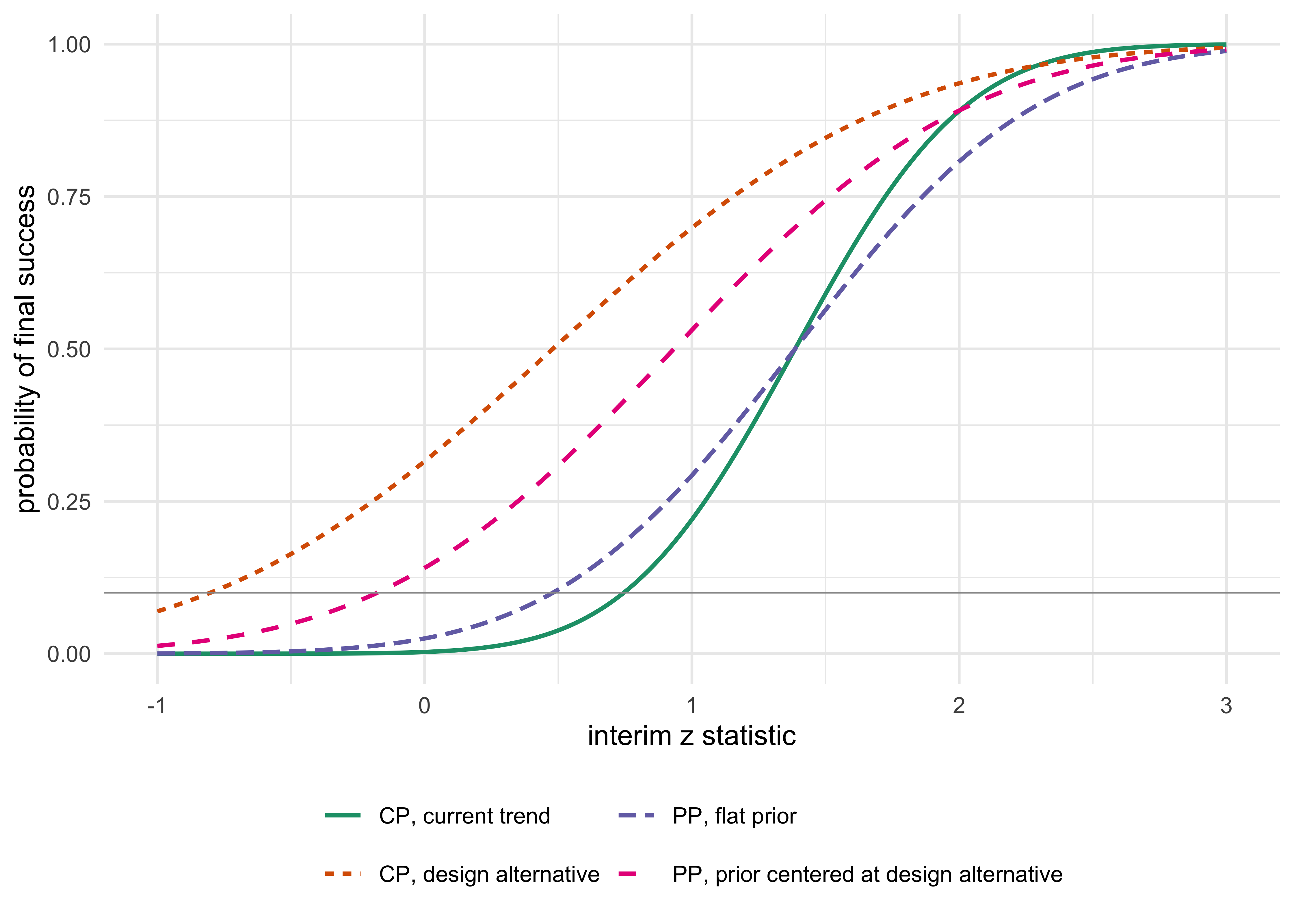
z <-seq(-1, 3, length.out =201)d <-rbind(data.frame(z, p =cond_power(z, t, xi_a), what ="CP, design alternative"),data.frame(z, p =cond_power(z, t, z /sqrt(t)), what ="CP, current trend"),data.frame(z, p =pp_normal(z, t), what ="PP, flat prior"),data.frame(z, p =pp_normal(z, t, xi_a, 1), what ="PP, prior centered at design alternative"))ggplot(d, aes(z, p, colour = what, linetype = what)) +geom_line(linewidth =0.8) +geom_hline(yintercept =0.10, colour ="grey60", linewidth =0.3) +scale_colour_brewer(palette ="Dark2") +labs(x ="interim z statistic", y ="probability of final success", colour =NULL, linetype =NULL) +theme_minimal() +theme(legend.position ="bottom") +guides(colour =guide_legend(nrow =2))
Figure 15.1: Conditional power under the design alternative, under the current trend, and the predictive probability of success under a flat prior and under a design-alternative prior N(3.24, 1), as a function of the interim z statistic at half the information (t = 0.5, one-sided alpha 0.025, design power 90%).
Figure 15.1 and Table 15.1 show the pattern. At \(Z_t = 1.0\) the flat-prior predictive probability is 0.293, between the two conditional power values (0.220 and 0.699, but nearer the trend) and a good deal more cautious than the design-alternative version. With a prior centered on the design alternative and unit variance (a prior worth as much information as the whole trial, which is a strong prior), the interim data at \(Z_t = 1.0\) give 0.531: the prior pulls the effect estimate up and the predictive probability with it. Neither number is the “right” one. They answer the question under different priors, which is why the prior must be pre-specified (Chapter 8) and why the sensitivity of the stopping decision to the prior belongs in the simulation report.
NoteTechnical note: the predictive distribution of the final statistic
Let \(B_t = Z_t\sqrt{t}\) be the interim B-value, with \(B_1 - B_t \mid \xi \sim N(\xi(1-t), 1-t)\) independent of \(B_t\). With prior \(\xi \sim N(\mu_0, \sigma_0^2)\) and \(B_t \mid \xi \sim N(\xi t, t)\), the posterior is \(\xi \mid B_t \sim N(\mu_p, v_p)\) with \(v_p = (t + 1/\sigma_0^2)^{-1}\) and \(\mu_p = v_p(B_t + \mu_0/\sigma_0^2)\). Then \(Z_1 = B_t + (B_1 - B_t)\) has predictive law \(N\big(B_t + (1-t)\mu_p,\; (1-t) + (1-t)^2 v_p\big)\). A flat prior (\(\sigma_0^2 = \infty\)) gives \(v_p = 1/t\), \(\mu_p = B_t/t\), and predictive mean \(B_t/t = Z_t/\sqrt{t}\) with variance \((1-t)/t\). The flat-prior predictive probability exceeds the current-trend conditional power when \(Z_t\) is below \(z_\alpha\sqrt t\) and falls short of it above, because the added variance helps when the trend is below the target and hurts when it is above.
The exact beta-binomial computation
For a binary endpoint no normal approximation is needed. Suppose \(n\) of the planned \(N\) patients are observed, with \(s\) responders, and the prior on the response probability is \(\mathrm{Beta}(a_0,b_0)\). The posterior is \(\mathrm{Beta}(a_0+s, b_0+n-s)\), and the number of responders \(X\) among the \(m = N-n\) remaining patients has the beta-binomial predictive distribution
\[
\Pr(X = x \mid s, n) = \binom{m}{x}\frac{B(a_0+s+x,\; b_0+n-s+m-x)}{B(a_0+s,\; b_0+n-s)}, \qquad x = 0,\dots,m,
\tag{15.3}\]
with \(B(\cdot,\cdot)\) the beta function. Each value of \(x\) completes a data set of \(N\) patients, to which the final success criterion can be applied directly, so the predictive probability is the sum of the beta-binomial probabilities of the \(x\) for which the criterion is met:
There is no integration and no simulation. The same construction for two arms takes a double sum over the future counts in each arm, with the posterior probability of superiority computed for each pair by adaptive numerical integration on the rank scale, cached across states (pp_two_arm in bayestrials); the predictive sum itself is exact.
A single-arm phase 2 example, with a fixed design first. The control response rate is \(p_0 = 0.20\), the target is \(p_1 = 0.40\), and the trial enrolls \(N = 40\) patients. With a \(\mathrm{Beta}(1,1)\) prior, the final criterion is \(\Pr(p > 0.20 \mid \text{data}) > 0.95\), which here works out to at least 13 responders of 40.
Show the R code
N <-40; p0 <-0.20; eta <-0.95succ <-pbeta(p0, 1+0:N, 1+ N -0:N, lower.tail =FALSE) > eta # succ[x + 1]: success with x respondersps <-c(0.20, 0.30, 0.40)knitr::kable(data.frame(p = ps, P =sapply(ps, function(p) sum(dbinom(0:N, N, p)[succ]))), digits =3,col.names =c("True response rate", "P(success)"))
Table 15.2: Probability of success of the fixed single-arm design (N = 40, criterion Pr(p > 0.20 | data) > 0.95, Beta(1,1) prior) at three true response rates.
True response rate
P(success)
0.2
0.043
0.3
0.423
0.4
0.871
The fixed design (Table 15.2) has type I error 0.043 and 87% power at \(p = 0.40\), which is a conventional phase 2 operating profile. The predictive probability at the interim answers a different question: after, say, 20 patients with 6 responders, how likely is the criterion to be met at 40?
Table 15.3: Predictive probability of meeting the final criterion (at least 13 responders of N = 40) for selected interim outcomes of the single-arm example.
Patients observed
Responders
Predictive probability
10
3
0.513
10
5
0.934
20
5
0.219
20
6
0.457
20
7
0.713
30
8
0.150
30
10
0.692
In Table 15.3, twenty patients with six responders (30%) gives a predictive probability of 0.457: a trial that is on course for an observed rate of 30% needs 13 of 40, and the remaining 20 patients have to deliver 7 more. Twenty patients with 5 responders gives 0.219; with 7 it gives 0.713. The predictive probability moves fast near the middle, and a single responder changes the picture at an interim of 20.
A time-to-event example
The normal-case formulas apply directly to an event-driven trial, where total information is \(D/4\) for \(D\) events (so the information fraction is \(D/D_{\max}\)) and the log hazard ratio has variance about \(4/D\). The worked example, with the predictive probability and the conditional power under the design effect and under the current trend side by side for four interim states, is in Section 18.4. The three summaries condition on different things (a fixed design effect, a fixed current estimate, and a posterior that averages over the effect), and which is more useful depends on how much the interim estimate is trusted against the design assumption; none is wrong, and the table there shows where they differ.
The same logic applies when the interim is combined with an earlier trial. In a continuous-endpoint program (an invented example), a skeptical posterior from phase 2 of mean 0.20 and standard deviation 0.115 is combined with a half-information interim of a pivotal trial (300 patients per arm at the interim, 600 per arm at the final analysis) that reports \(\hat\theta_1 = 0.15\) with standard error \(\sqrt{2/300}\).
Show the R code
w <-c(1/0.115^2, 300/2) # precisions: phase 2 posterior, interim datam2 <-sum(w *c(0.20, 0.15)) /sum(w); s2 <-1/sqrt(sum(w))# final estimate = (theta1 + theta2)/2, need z >= 2.02 at SE sqrt(2/600)thr <-2*2.02*sqrt(2/600) -0.15# required value of the second-half estimatepp_prog <-pnorm((m2 - thr) /sqrt(s2^2+2/300))
The combined posterior has mean 0.167 and standard deviation 0.067, and the predictive probability of crossing the final boundary of 2.02 is 0.79, high enough to continue. An interim estimate near zero would have started a futility discussion, and the predictive probability, not the conditional power at the design effect, would have been the quantity to discuss. The regulator analyzes the pivotal trial on its own data, so the type I error is controlled by that analysis; the sponsor deciding whether to continue may use everything it knows. These are different decisions, and they can use different priors.
15.3 The traditional phase 2 design, and where Bayesian monitoring started
The single-arm phase 2 trial is a widely used early efficacy design in oncology, and its traditional form is older than the predictive probability designs that follow. A response rate \(p\) is judged against an uninteresting rate \(p_0\) and a target rate \(p_1\). Gehan (1961) proposed a first stage that stops when there are no responses, and Fleming (1982) a one-sample multiple testing procedure with early stopping. The design most protocols use is the two-stage design of Simon (1989): enroll \(n_1\) patients and stop for futility if at most \(r_1\) respond; otherwise enroll to a total of \(n\) and declare the drug promising if more than \(r\) respond. Among the pairs of stages that meet the stated type I error and power, the optimal design is the one with the smallest expected sample size under \(p_0\). Both error rates are exact binomial sums, so the design is computed, not simulated.
Show the R code
s1 <-simon_optimal(0.2, 0.4, 0.05, 0.80)tb3 <-lee_liu_table(N, p0, c(10, 20, 30), th_fut =0.05, th_eff =0.95, eta = eta)ll0 <-lee_liu_oc(N, 0.2, tb3, p0, eta); ll1 <-lee_liu_oc(N, 0.4, tb3, p0, eta)s2 <-simon_optimal(0.2, 0.4, ll0[[1]], ll1[[1]])oc_row <-function(s) c(simon_oc(s$n1, s$r1, s$n, s$r, 0.2)[[1]], simon_oc(s$n1, s$r1, s$n, s$r, 0.4)[[1]], s$EN, simon_oc(s$n1, s$r1, s$n, s$r, 0.4)[[2]], s$n)ph2 <-rbind(c(sum(dbinom(0:N, N, 0.2)[succ]), sum(dbinom(0:N, N, 0.4)[succ]), N, N, N),oc_row(s1), oc_row(s2), c(ll0[[1]], ll1[[1]], ll0[[2]], ll1[[2]], N))knitr::kable(data.frame(design =c(paste0("Fixed, ", which(succ)[1] -1, " or more of ", N), "Simon optimal, alpha 0.05, power 0.80", "Simon optimal, matched to the three-look design", "Predictive probability, three looks (next section)"), ph2),digits =c(0, 3, 3, 1, 1, 0), col.names =c("Design", "Type I error", "Power", "Expected N at p0", "Expected N at p1", "Maximum N"))
Table 15.4: Single-arm phase 2 designs for p0 = 0.20 and p1 = 0.40, with exact type I error (at p0), power (at p1) and expected sample size at p0 and at p1. Simon’s optimal two-stage design is shown at the conventional error rates (0.05, 0.80) and at the error rates of the three-look predictive probability design of the next section.
Design
Type I error
Power
Expected N at p0
Expected N at p1
Maximum N
Fixed, 13 or more of 40
0.043
0.871
40.0
40.0
40
Simon optimal, alpha 0.05, power 0.80
0.050
0.800
20.6
37.9
43
Simon optimal, matched to the three-look design
0.048
0.870
26.8
43.6
46
Predictive probability, three looks (next section)
0.048
0.867
26.6
27.2
40
At the conventional error rates the optimal Simon design stops after 13 patients if at most 3 respond and otherwise continues to 43, declaring the drug promising if more than 12 respond; its type I error is 0.050, its power 0.800, and its expected sample size under \(p_0\) is 20.6 (Table 15.4), which reproduces the published table of Simon (1989). It has a single look and stops for futility only. Matched to the error rates of the three-look predictive probability design of Section 15.4, the optimal Simon design is 5/21 and 13/46, with expected sample size 26.8 under \(p_0\), against 26.6 for the three-look design: the two are close. Under \(p_1\) the expected sample size is 27.2 for the three-look design against 43.6 for the matched Simon design, and that is the main gain: the possibility of stopping for efficacy. The other gain is a smaller maximum sample size (40 against 46). Under the null the reduction in the expected sample size is small.
The Bayesian single-arm designs came in two steps. Herson (1979) proposed stopping on the predictive probability of a positive final result. Thall and Simon (1994) monitored on the posterior probability that the response rate exceeds a target and chose the thresholds by their frequentist operating characteristics; Thall, Simon, and Estey (1995) extended the idea to several outcomes, and Heitjan (1997), Tan and Machin (2002) and the BOP2 design of Zhou, Lee, and Yuan (2017) are later versions. The next section is the predictive probability form of the same idea.
15.4 Predictive probability monitoring for phase 2
Lee and Liu (2008) turned the predictive probability of success into a two-threshold monitoring design for phase 2 with a printed stopping table. Related treatments include Johns and Andersen (1999) (phase 2 and 3), Dmitrienko and Wang (2006) (normal and time-to-event endpoints, with the link to conditional power) and Saville et al. (2014) (practical interim use). The idea is the same as the predictive probability futility rule of Section 15.2, written in the units a phase 2 clinician uses: after each cohort, compute the predictive probability that the trial will end in success. Stop for futility if it is below a lower threshold \(\eta_L\), stop for efficacy if it is above an upper threshold \(\eta_U\), and otherwise continue. At the maximum sample size the trial declares success if the posterior probability criterion \(\Pr(p > p_0 \mid \text{data}) > \eta\) is met. Because the rule is a function of \((n, s)\) only, the decision for every possible interim outcome can be tabulated before the trial begins and printed in the protocol. Real trials use the same logic: the BNT162b2 trial planned to stop for futility if the predictive probability of success fell to 5% or less, and the DAWN stroke trial used predictive probability for both futility and expected success (Section 15.10).
For the example above with \(\eta_L = 0.05\), \(\eta_U = 0.95\), and final threshold \(\eta = 0.95\), and with looks after 10, 20 and 30 patients:
Show the R code
tab <-lee_liu_table(N, p0, c(10, 20, 30), th_fut =0.05, th_eff =0.95, eta = eta)knitr::kable(tab, col.names =c("Patients observed", "Stop for futility if responders at most", "Stop for efficacy if responders at least"))
Table 15.5: Stopping table of the three-look predictive probability design (N = 40, p0 = 0.20): stop for futility at or below the first number of responders, and for efficacy at or above the second.
Table 15.6: Exact operating characteristics of the three-look design and of the same design with looks every five patients: probability of declaring success and expected sample size.
True response rate
Looks
P(success)
Expected N
0.2
Three
0.048
26.6
0.2
Seven
0.057
22.6
0.4
Three
0.867
27.2
0.4
Seven
0.862
23.2
This is the table a protocol prints. The three-look design stops for futility after 10 patients only if there are no responders, after 20 if there are three or fewer, and after 30 if there are seven or fewer; it stops for success after 10 with six or more responders, after 20 with nine or more, and after 30 with twelve or more. The operating characteristics follow from exact enumeration of all paths, not from simulation: the probability of declaring success is 0.048 under the null rate (compared with 0.043 for the fixed design) and 0.867 at \(p = 0.40\) (0.871 for the fixed design), with an expected sample size of about 27 patients under either, against 40 for the fixed design.
Three observations. First, power is essentially unchanged and the sample size falls by roughly a third. Second, the expected sample size is almost the same under the null and the alternative (26.6 and 27.2), because efficacy stops under the alternative offset futility stops under the null. Third, the type I error is not guaranteed to stay at the fixed-design value once efficacy stopping is allowed: with looks every five patients the null success probability rises to 0.057 (power 0.862, expected \(N\) 22.6 to 23.2), above 0.043, so the thresholds have to be recalibrated by exact enumeration or simulation (Chapter 14). Phase 2 trials often accept a type I error of 0.05 to 0.10 by design; a confirmatory trial targets 0.025 one-sided.
What the predictive probability design is, and is not
Predictive probability monitoring is a Bayesian way of computing a stopping boundary and a frequentist way of judging it. The decisions are made on a Bayesian quantity. The design is accepted or rejected on its operating characteristics under simulated truth. For a trial that adapts only by stopping, the realized design is a group sequential design with an unusual, data-driven boundary shape, and its probability of success under any true \(p\) is exact. This is how the FDA Bayesian draft expects a Bayesian design to be defended, and it is why the draft’s demand for pre-specified thresholds and simulation is no obstacle: the table above is the pre-specification.
The approximation of Marion et al. (2025) shows that the exact calculation can be avoided in normal-approximation settings. If \(q_n\) is the current posterior probability of superiority, \(r\) the information fraction and \(\eta\) the final threshold, then
which needs only the current posterior probability and the information fraction. The approximation assumes a Gaussian posterior and test statistic, and with a flat prior \(r\) is the share of the final information accrued, \(I_n/I_N\). With an informative normal prior of precision \(J_0\) the fraction for the posterior-threshold formula is \((J_0 + I_n)/(J_0 + I_N)\) rather than \(I_n/I_N\), and with longitudinal outcomes \(r\) is the fraction of final information carried by the observed data, not the fraction of patients enrolled (Marion et al. 2025). In the binary example of the working paper by Polson and Sokolov (cited below as SIM) (Polson and Sokolov 2026), with ten looks, thresholds 0.95 and 0.05 and final threshold 0.975, the approximation and the exact computation differ by 0.013 in mean absolute error across all interim states, and at most 9.0% of states receive different monitoring actions. Run through the full trial, the two give null success probabilities of 0.042 and 0.041, powers of 0.932 and 0.928, and expected sample sizes of 48.2 and 47.6 per arm. The approximation is good enough for planning, but the numbers also show that it is a design component to validate rather than an identity: where the final decision depends on a fine threshold, use the exact calculation.
The economic threshold \(PP^*\)
The thresholds 0.05 and 0.95 are conventions. A decision-theoretic reading ties the futility threshold to money. Suppose a false go costs \(c_3\), the expected cost of a failed phase 3, and a missed active drug forfeits \(V\), its expected net value if developed. Continuing from the interim costs the remaining patients, \(m c_2\), and \(\rho\) is the probability that phase 3 succeeds given a phase 2 success. The myopic rule continues if \(\mathrm{PP}\,[\rho V - (1-\rho) c_3] > m c_2\), so the continuation threshold is
\[
\mathrm{PP}^* = \frac{m c_2}{\rho V - (1-\rho) c_3},
\tag{15.6}\]
which is small when the drug is valuable and the remaining phase 2 is cheap. The numbers below are invented for teaching, not taken from a real program.
Table 15.7: Economic futility threshold PP* for two invented drugs (values in millions of dollars): a valuable drug and a drug in a crowded indication. A negative denominator means a phase 2 success does not justify going on to phase 3.
V
rho
c3
m c2
rho V - (1 - rho) c3
PP*
Viable
500
0.5
150
2
175
0.011
TRUE
100
0.5
150
2
-25
-0.080
FALSE
For the valuable drug, \(\mathrm{PP}^* =\) 0.011, so the conventional 0.05 is more aggressive than the economics justify: a sponsor following expected value would keep enrolling at an interim where the predictive probability is 0.02. For the crowded indication the denominator is negative, -25, which means a phase 2 success leads to a phase 3 of negative expected value and the trial should not be running at all. The lesson is not that 0.011 is the right number but that the futility threshold is a consequence of the economics and should be derived from them, then judged by operating characteristics like any other threshold (Chapter 14). The toxicity counterpart, a continuous Bayesian stopping rule for excess toxicity, is in Chapter 13.
15.5 The Goldilocks design: two predictive probabilities
Phase 2 monitoring asks one question: will the trial succeed at its maximum size? A confirmatory trial with a long follow-up asks two, and the Goldilocks sample size design of Broglio, Connor, and Berry (2014) separates them (Section 14.7 introduces it as a design chosen by simulation; this section gives the construction). The trial has a maximum sample size \(N_{\max}\) per arm and enrolls continuously. Because the primary endpoint is observed after a delay (say at week 12), at an interim look some enrolled patients have outcomes and some are still pending. At each look the design computes two predictive probabilities, both for the final success criterion, say \(\Pr(p_1 - p_0 > 0 \mid \text{data}) > 0.975\):
\(\mathrm{PP}_{\text{stop}}\): the probability of success if enrollment stops now and the pending patients are followed to complete their outcomes. Only the pending outcomes are unknown.
\(\mathrm{PP}_{\max}\): the probability of success if the trial continues to the maximum sample size, where every patient not yet observed (pending or not yet enrolled) is unknown.
The decisions are: stop enrolling for expected success if \(\mathrm{PP}_{\text{stop}}\) is high (the trial has already answered the question, and the pending patients will confirm it); stop for futility if \(\mathrm{PP}_{\max}\) is low (even the full sample is unlikely to succeed); otherwise, keep enrolling. The “not too big, not too small” name refers to the sample size that the data pick, between the two limits. The two probabilities are different questions with different thresholds, and the design adjusts the sample size to both. The full design of Broglio and colleagues, as summarized in Section 14.7, also has an immediate-success rule that declares success without following the pending patients when \(\mathrm{PP}_{\text{stop}}\) passes a higher threshold; this chapter includes only the stop-enrollment rule above.
Show the R code
# Two arms, Nmax = 100 per arm. At the look: 60 enrolled per arm, 50 with outcomes, 10 pending.sc <-data.frame(label =c("treatment ahead", "modest lead", "narrow lead", "no difference"),s1 =c(30, 24, 22, 18), s0 =c(15, 15, 19, 18))sc$post <-with(sc, prob_superior(1+ s1, 51- s1, 1+ s0, 51- s0))sc$PP_stop <-with(sc, mapply(pp_two_arm, s1, 50, s0, 50, 10, 10, 0.975)) # only the 10 pending per arm unknownsc$PP_max <-with(sc, mapply(pp_two_arm, s1, 50, s0, 50, 50, 50, 0.975)) # 10 pending + 40 unenrolled unknownsc$action <-with(sc, ifelse(PP_stop >0.95, "stop enrolling", ifelse(PP_max <0.05, "stop for futility", "continue")))knitr::kable(sc, digits =3, col.names =c("Scenario", "Treatment responders", "Control responders", "Posterior P(superior)", "PP stop", "PP max", "Action"))
Table 15.8: Goldilocks decision at the look (60 enrolled per arm, 50 with outcomes, maximum 100 per arm) for four interim scenarios: responders in each arm, posterior probability of superiority, the two predictive probabilities and the resulting action.
Scenario
Treatment responders
Control responders
Posterior P(superior)
PP stop
PP max
Action
treatment ahead
30
15
0.999
0.999
0.990
stop enrolling
modest lead
24
15
0.966
0.545
0.735
continue
narrow lead
22
19
0.727
0.001
0.133
continue
no difference
18
18
0.500
0.000
0.022
stop for futility
The four rows of Table 15.8 show the logic. With 30 of 50 against 15 of 50 the posterior probability of superiority is already 0.999, \(\mathrm{PP}_{\text{stop}}\) is 0.999, and the design stops enrolling; completion is predicted to meet the success criterion with probability about 0.999, although unfavorable pending outcomes could reverse the decision. The modest lead (24 against 15, posterior probability 0.966) is not yet there: \(\mathrm{PP}_{\text{stop}}\) is 0.545, \(\mathrm{PP}_{\max}\) is 0.735, and the design keeps enrolling. The narrow lead of 22 against 19 gives \(\mathrm{PP}_{\max} = 0.133\), above the futility floor of 0.05, so the trial continues but is in trouble. Equal rates at 18 of 50 give \(\mathrm{PP}_{\max} = 0.022\) and the design stops for futility.
Two cautions, both of the kind a regulator raises. The thresholds (0.95 and 0.05 here are illustrative) must be calibrated by simulation so that the overall type I error is controlled (Section 14.4 shows this for the four-look example of Chapter 14, where the flat posterior threshold of 0.975 becomes \(c = 0.9907\)), and the look frequency and the delay length change the calibration. And stopping enrollment when the predictive probability of success is high is an efficacy decision: it spends type I error just as a group sequential efficacy boundary does (Chapter 14).
The same two questions run through the DAWN stroke trial (Section 15.10); I-SPY 2 uses a single predictive probability, that of success in a follow-on phase 3 trial. The Goldilocks design replaces three separate traditional elements (an interim efficacy boundary, a futility boundary, and a sample size re-estimation) with one pre-specified rule, and its operating characteristics are what justify it. It also has a price: the sample size is random, so budgets and supply have to be planned for the maximum and the expected sample size reported alongside it.
15.6 Backward induction: the Bayes-optimal stopping rule
Predictive probability monitoring is a rule with thresholds that the designer chooses and calibrates. A natural question is whether a best rule exists, for a stated loss. For a sequential decision problem with a finite horizon the answer is yes, and it can be found by working backward from the end. The method is backward induction, or dynamic programming (Bellman 1957). Sequential analysis itself goes back to Wald (1947), and Bayes sequential solutions by backward induction to Arrow, Blackwell, and Girshick (1949). Anscombe (1963) and Colton (1963) cast the trial as a Bayesian decision problem over a patient horizon, and Berry and Ho (1988) derived clinical-trial stopping boundaries by backward induction; Lewis and Berry (1994) evaluated such designs by their frequentist operating characteristics, the stance of this book. Later work includes Carlin, Kadane, and Gelfand (1998), Cheng and Shen (2005) and P. Müller et al. (2007) for sequential trials with a sufficient statistic; Brockwell and Kadane (2003) gave a gridding method for the normal model and Jiang, Lee, and Müller (2013) combined it with response-adaptive randomization. The presentation below follows SIM (Polson and Sokolov 2026).
The decision problem
A two-arm trial with binary outcomes enrolls one pair of patients at a time, one per arm, up to a maximum of \(T\) pairs. After \(k\) pairs, the trial can stop and declare a winner, or pay a cost \(\kappa\) for one more pair. A stopping loss records the consequences of the terminal decision, and the continuation cost records the consequences of waiting. Two stopping losses are useful.
The utility version stops for treatment when the posterior mean effect \(\hat\theta_k\) is positive and for control otherwise, with stopping value \(h_k = -\max(0, \hat\theta_k)\), the negative of the expected benefit of the chosen arm. It has no separate cost for a false positive, so it is a decision rule for patient benefit, not an evidence rule, and it is deliberately aggressive under the null.
The classification version fixes the losses \(L_{\mathrm{FP}}\) for declaring superiority when it is absent and \(L_{\mathrm{FN}}\) for failing to declare it when it is present. With \(q_k = \Pr(p_1 > p_0 \mid \text{data}_k)\), \(\gamma = L_{\mathrm{FP}}/(L_{\mathrm{FP}}+L_{\mathrm{FN}})\) and \(\kappa\) the cost per pair normalized by \(L_{\mathrm{FP}}+L_{\mathrm{FN}}\), the Bayes stopping loss and action are
A loss ratio of \(L_{\mathrm{FP}} : L_{\mathrm{FN}} = 39 : 1\) gives \(\gamma = 0.975\), which is the Bayesian reading of one-sided 0.025: a false positive is 39 times worse than a false negative. This ratio is illustrative; the elicitation of the real ratio is the part of the design that belongs to clinicians, sponsors and regulators, not to the statistician.
The sufficient-statistic reduction
The data history up to pair \(k\) is a sequence of \(4^k\) possible outcome patterns. The posterior depends on the history only through the success counts \((s_1, s_0)\) and \(k\), because the beta-binomial model has sufficient statistics. With the prior \(\mathrm{Beta}(a_{0i}, b_{0i})\) in arm \(i\), the predictive probability of the next outcome in that arm is
so the future depends on the past only through \((s_1, s_0, k)\). This is the sufficient-statistic reduction: the decision tree, which grows exponentially, collapses to a lattice with \((k+1)^2\) states at stage \(k\), and the trial’s whole future is a function of where on the lattice it stands.
With \(V_k(s_1, s_0)\) the minimum expected loss from state \((s_1, s_0)\) at stage \(k\) onward, the Bellman equation is
for \(0 \le k < T\), with \(V_T = h_T\) at the horizon (the trial is forced to decide). The first term is the loss from stopping now. The second is the cost of one more pair plus the expected loss at the next stage, averaged over the four outcomes of the next pair with the predictive probabilities of Equation 15.8. The minimum of the two is the best that can be done from here, and the argument that achieves it is the optimal action. One computes \(V_T\) first, then \(V_{T-1}\) from it, and so on back to \(V_0\): backward induction.
NoteTechnical note: why the optimal policy is a function of the lattice state, and its cost
Proposition (SIM, Appendix). For fixed prior parameters and horizon \(T\), the optimal policy at stage \(k\) is a function of \((s_1, s_0, k)\) only, and the recursion in Equation 15.9 evaluates \(\sum_{k=0}^{T}(k+1)^2 = (T+1)(T+2)(2T+3)/6 = O(T^3)\) states, each in constant time.
Proof sketch. By conjugacy the posterior at stage \(k\) is \(\mathrm{Beta}(a_{0i} + s_i, b_{0i} + k - s_i)\) in each arm, so \((s_1, s_0, k)\) is a Markov sufficient state for the future. The one-step predictive probabilities of Equation 15.8 depend on no other feature of the history, so the continuation value is a function of the state, and so is the minimum over the two actions. Each update is the arithmetic of four lookups of \(V_{k+1}\). Summing the number of states over stages gives the cubic count. For \(T = 200\) pairs, about 2.7 million states. \(\square\)
For normal data with known variance the same argument holds with the posterior mean as the scalar state, and the lattice is replaced by a grid of the posterior mean; Brockwell and Kadane (2003) used 12,000 grid points on \([-6, 6]\).
The result is exact for the binary endpoint: no simulation, no approximation, no quadrature. The only approximation in the classification version is numerical, the computation of \(q_k\) for each state, which is a one-dimensional integral that bayestrials evaluates by the same adaptive rank-scale integration, with caching. The classification-loss version is implemented in backward_induction of the bayestrials package, together with an exact forward propagation (forward_oc) that returns the probability of declaring superiority and the expected sample size under any true pair \((p_1, p_0)\).
Show the R code
nT <-60; gamma <-0.975scen <-list(null =c(0.30, 0.30), target =c(0.55, 0.30), small =c(0.45, 0.30))policies <-lapply(c(`0.0001`=1e-4, `2e-05`=2e-5), backward_induction, T = nT, loss ="class", gamma = gamma)fx <-sapply(scen, function(p) fixed_oc(nT, gamma, p[1], p[2]))bi <-do.call(rbind, lapply(names(policies), function(nm) { o <-sapply(scen, function(p) forward_oc(policies[[nm]], p[1], p[2]))data.frame(design =paste("Bayes-optimal, kappa =", nm), quantity =c("P(declare treatment)", "E[N per arm]"), o, check.names =FALSE)}))tabbi <-rbind(data.frame(design ="Fixed, 60 per arm", quantity ="P(declare treatment)", t(fx), row.names =NULL), bi)knitr::kable(tabbi, digits =3, row.names =FALSE, col.names =c("Design", "Quantity", "Null", "Target", "Small effect"))
Table 15.9: Operating characteristics of the fixed 60-per-arm design and of two Bayes-optimal classification-loss policies (gamma = 0.975, cost kappa per pair) under the null (0.30, 0.30), the target (0.55, 0.30) and a small effect (0.45, 0.30): probability of declaring treatment better and expected sample size per arm.
Design
Quantity
Null
Target
Small effect
Fixed, 60 per arm
P(declare treatment)
0.024
0.806
0.393
Bayes-optimal, kappa = 0.0001
P(declare treatment)
0.023
0.708
0.335
Bayes-optimal, kappa = 0.0001
E[N per arm]
19.388
34.996
33.370
Bayes-optimal, kappa = 2e-05
P(declare treatment)
0.024
0.790
0.384
Bayes-optimal, kappa = 2e-05
E[N per arm]
30.237
45.880
46.147
In Table 15.9, at a cost of \(2\times10^{-5}\) per pair, the classification-loss policy declares superiority with probability 0.024 under the null (the fixed design: 0.024), 0.790 at (0.55, 0.30) (fixed: 0.806), and 0.384 at (0.45, 0.30) (fixed: 0.393). Its expected sample size under the target alternative is 45.9 pairs, against 60 for the fixed design. At the target alternative the Bayes policy gives power 0.790 against 0.806 for the fixed design, at 24% fewer patients on average: a small loss of power for a substantial saving, not equal operating characteristics. Raising the cost to \(10^{-4}\) makes continuation more expensive: power at the target falls to 0.708 and expected sample size to 35.0 pairs. This is the power frontier, the trade-off between the expected number of patients and the probability of a correct declaration, indexed by the cost \(\kappa\). A designer calibrates \(\kappa\) so that the frontier passes through the operating characteristics the protocol promises: that paper does this for a maximum of 100 per arm and finds the cost at which the null declaration probability is held below 0.05 over a grid of 99 equal-rate scenarios and the power at (0.55, 0.30) is at least 0.90 (Polson and Sokolov 2026). That calibrated policy has a largest null declaration probability of 0.026 (slightly above 0.025, because the SIM calibration holds it below 0.05 over the grid), target power 0.903 and expected sample size 54.3 pairs, against 100 for the fixed design with 100 per arm.
Show the R code
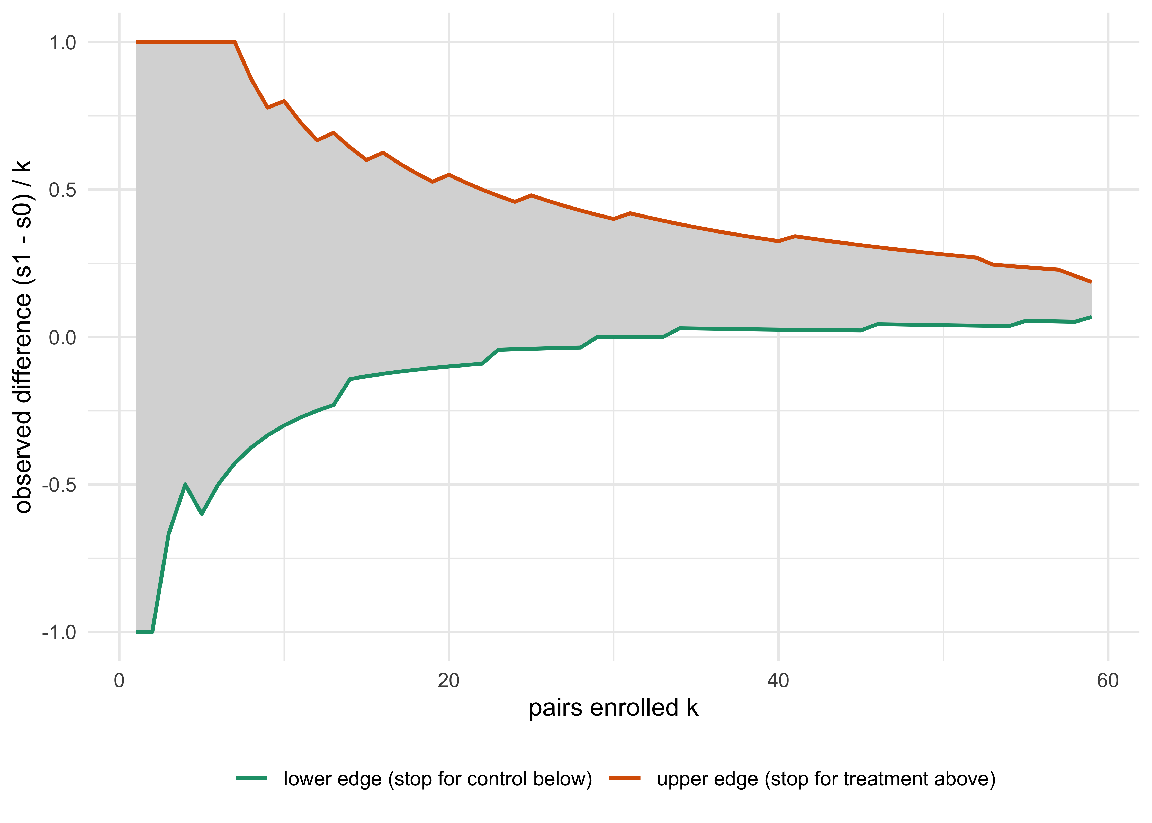
st <- policies[["2e-05"]]$stopreg <-do.call(rbind, lapply(1:(nT -1), function(k) { w <-which(!st[[k +1]], arr.ind =TRUE)if (nrow(w) ==0) return(NULL) d <- (w[, 1] - w[, 2]) / k; data.frame(k = k, lo =min(d), hi =max(d)) }))ggplot(reg, aes(k)) +geom_ribbon(aes(ymin = lo, ymax = hi), fill ="grey85") +geom_line(aes(y = hi, colour ="upper edge (stop for treatment above)"), linewidth =0.8) +geom_line(aes(y = lo, colour ="lower edge (stop for control below)"), linewidth =0.8) +scale_colour_brewer(palette ="Dark2") +labs(x ="pairs enrolled k", y ="observed difference (s1 - s0) / k", colour =NULL) +theme_minimal() +theme(legend.position ="bottom")
Figure 15.2: Continuation region of the Bayes-optimal classification-loss policy (T = 60 pairs, gamma = 0.975, cost 2e-5 per pair), shown as the range of the observed difference in success proportions among continuation states at each stage (a projection: the full policy is indexed by the pair of success counts, and states with the same difference can have different actions). Continuation states lie within the shaded envelope between the two edges; the action at a particular point requires both success counts. Above the upper edge the trial stops for treatment, below the lower edge for control.
Figure 15.2 shows the familiar funnel. Early in the trial a large observed difference is needed to stop for treatment (0.8 after 10 pairs, 0.55 after 20, 0.4 after 30, 0.28 after 50), because a few patients say little; the trial stops for control once the observed difference falls to about 0 after 30 pairs. The region closes as \(k\) approaches the horizon, because the trial is forced to decide at \(T\) whatever happens. The optimal rule has the shape of a group sequential boundary, with efficacy and futility stopping, but it is derived from a loss and a cost, not from an error-spending function. The projection onto the observed difference is only a summary: the full policy is indexed by \((s_1, s_0, k)\), and states with the same difference can have different decisions.
What backward induction does and does not do
Three honest limits. First, a Bayes-optimal rule is optimal for the stated loss under the stated prior, and the loss ratio and cost are inputs somebody has to choose. A decision-theoretic submission should justify its loss function, prior, success criterion, and operating characteristics. For the error-calibrated approach used in this book, the route from one to the other is the calibration above: choose \(\gamma\) and \(\kappa\), compute the policy, simulate (or enumerate) its operating characteristics under the full range of scenarios, and adjust until they meet the protocol targets. The decision-theoretic framing is a way of generating a good design; the frequentist operating characteristics are how it is judged (Chapter 14).
Second, the utility-only version shows what happens when a loss does not penalize false positives. In SIM’s calculation, with \(\kappa = 0.0005\) and a maximum of 100 per arm, utility-only backward induction declares treatment better with probability 0.513 under the null (Monte Carlo standard error 0.005) and 0.98 at the large effect, with an expected sample size of only 14.4 per arm. It is a good rule for choosing the arm that gives patients the best outcomes, and a useless rule for a confirmatory claim: its “null error” is a treatment-choice probability, not a type I error. The classification version, with \(\gamma = 0.975\), has a null declaration probability of 0.026, and its expected sample size at the large effect is 54.3 per arm with power 0.903. The loss function is the design.
Third, the lattice assumes that outcomes are observed before the next decision, balanced allocation, and no pending patients. Delayed outcomes enlarge the state to include the pending counts, which is the setting of the Goldilocks design above, and response-adaptive allocation adds the allocation decision to the action set (Chapter 16). Those extensions are what make exact dynamic programming harder; the sufficient-statistic reduction is what makes it feasible at all.
A single-arm example
The two-arm lattice above has a one-arm counterpart that can be printed as a table. A single-arm trial enrolls patients one at a time, up to 60, with a Beta(3, 7) prior on the response rate \(p\), centered at a standard-of-care rate \(p_0 = 0.3\). Each patient costs \(c = 0.002\) in utility units. When the trial stops at \(n\) patients with \(x\) responders it adopts the drug if the posterior mean exceeds \(p_0\), earning \(M(\hat p - p_0)\) with \(M = 10\) standing for the population of future patients, and abandons it otherwise. With \(\hat p_n = (3 + x)/(10 + n)\), the value \(V_n(x)\) of state \((n, x)\) satisfies
solved backward from \(V_{60}\). This is an invented teaching example with no regulatory standing: it has no type I error target.
Show the R code
st <-decide_stop_single_arm(p =c(0.2, 0.3, 0.45))knitr::kable(st$table, col.names =c("Patients n", "Continue from x =", "Continue to x =", "Adopt if x at least"))
Table 15.10: Optimal stopping of the single-arm problem (Beta(3, 7) prior, horizon 60, M = 10, cost 0.002 per patient): the trial continues while the number of responders lies in the given range, and adopts the drug on stopping at or above the last column.
Table 15.11: Exact operating characteristics of the single-arm optimal stopping rule: probability of adopting the drug and expected number of patients at three true response rates.
True response rate
P(adopt)
Expected N
0.20
0.053
24.8
0.30
0.496
32.3
0.45
0.976
19.1
The continuation region of Table 15.10 is a band around the adoption boundary that narrows as the trial proceeds, because each additional patient moves the posterior less and so is worth less. Outside the band the decision is clear enough that more data cannot pay for themselves. The operating characteristics, computed exactly by forward propagation, are small where the stakes are large and large only where the two actions are nearly equivalent: at \(p = 0.2\) the drug is adopted with probability 0.053 after 24.8 patients on average, at the boundary \(p = 0.3\) with probability 0.50 after 32.3, and at \(p = 0.45\) with probability 0.976 after 19.1. This is the general shape of Bayes sequential designs. The same caveat applies as above: the loss and the cost are inputs, and a regulator reviews the operating characteristics (or, under the other routes of the FDA draft, the posterior or benefit-risk criterion), not the loss.
15.7 Comparing the designs
SIM puts five specifications on a common footing, a two-arm trial with a maximum of 100 patients per arm, \(p_0 = 0.30\) and a large effect of \(\theta = 0.25\), and reports power and expected sample size per arm (Polson and Sokolov 2026). The rows are different specifications, with different objectives and monitoring schedules, so the table is a description of each and not a ranking of methods.
Table 15.12: Power and expected sample size at \(\theta = 0.25\) (SIM, maximum 100 per arm; all rows are 10,000 simulated trials per scenario except the classification-loss row, which is exact enumeration, where SIM’s simulation reports power 0.911. Realized null declaration probabilities: 0.033 for the O’Brien-Fleming-shaped rule (not recalibrated for discrete data), 0.028 for the fixed Wald test, 0.042 for predictive probability monitoring and 0.026 for classification-loss backward induction, but 0.513 for the utility-only rule, which is a treatment-choice probability).
Design
Power at \(\theta = 0.25\)
Expected \(N\) per arm
Fixed sample, one-sided Wald test
0.96
100
O’Brien-Fleming-shaped rule, five looks (efficacy only)
0.96
64.8
Predictive probability monitoring, ten looks (thresholds 0.95 and 0.05, final 0.975)
Three lessons. The traditional group sequential design, fixed at one sample size and efficacy-only, cuts the expected sample size from 100 to 64.8 per arm at this large effect with simulated power unchanged at 0.96: the Bayesian predictive designs are not the first to stop early. That comparator is an approximate O’Brien-Fleming-shaped rule with boundary \(\Phi^{-1}(0.975)\sqrt{5/j}\), not recalibrated for discrete data, and its realized null rejection probability is 0.033 against 0.028 for the fixed Wald test, so the comparison is not calibrated and no claim of a costless saving in power follows. The predictive probability and classification-loss designs go further because they also stop for futility, at a cost in power (0.93 and 0.90 against 0.96) that the calibration can trade back. And the utility-only rule shows that the objective changes everything: a rule that stops after 14 patients per arm and is right 98% of the time at the large effect is also wrong half the time under the null.
The honest reading of Table 15.12 is that backward induction does not “beat” group sequential monitoring. It chooses a rule for a stated loss, and the rule, once calibrated to the same operating characteristics, is in the family of the others. What the decision framing adds is the explicit price: the cost per patient and the loss per error are design parameters, where the group sequential design hides them in the choice of spending function.
15.8 Side by side: what changes in the protocol
Table 15.13: Interim monitoring and stopping, traditional and Bayesian predictive.
Traditional
Bayesian predictive
Interim quantity
Conditional power at the design alternative or the current trend; interim \(Z\) against a boundary
Predictive probability of final success (posterior-averaged), or posterior probability
Treatment of uncertainty in \(\xi\)
None: \(\xi\) is fixed at a chosen value
Averaged over the posterior; requires a prior
Futility
Non-binding boundary or conditional power threshold; adding it to an unchanged success rule cannot inflate the type I error
Threshold on PP (for example 0.05 to 0.10); the same holds when the success rule is unchanged, and the efficacy threshold is calibrated with the futility rule in place
Efficacy stopping
Alpha spending function (O’Brien-Fleming, Lan-DeMets)
Threshold on PP or posterior probability; calibrated by simulation
Sample size change
Blinded re-estimation; combination or conditional-error tests; promising zone
Goldilocks stopping of accrual; sample size is data-driven within a pre-specified maximum
Optimal rule
Group sequential designs optimized for expected sample size
Backward induction for a stated loss and cost
What the regulator asks
Spending function, boundaries, type I error
Thresholds, prior, simulated type I error and power, expected \(N\), sensitivity to prior and delay
What stays the same
The final test criterion, the type I error target (0.025 one-sided), the pre-specification, the walled-off DMC
The two approaches agree numerically in simple cases: with a flat prior and a large trial, the predictive probability of success at an interim is a function of the same \(Z_t\) and \(t\) as conditional power under the current trend, and the flat-prior posterior probability of benefit at the end is approximately one minus the one-sided \(p\)-value (Chapter 7). What the Bayesian design adds is the language, the prior, the forward-looking quantity that clinicians understand, and the framework for optimization. What it does not add is a lower bar.
When is the traditional design the better choice? A single interim for futility with a non-binding rule is simple, well understood by every DMC and regulator, and needs no prior and no simulation beyond the standard group sequential software. If the DMC will take its decision on clinical grounds, the extra machinery of a predictive probability rule has no one to use it. Where the decision is not a single stop-or-go but a sequence (several looks, a pending-outcome structure, a platform with many arms), the predictive design earns its complexity.
TipIn the protocol
A predictive monitoring section should state, before any outcome data are seen:
The final success criterion in full (for example, \(\Pr(p_1 - p_0 > 0 \mid \text{data}) > 0.975\) at \(N_{\max}\)) and the prior used to compute the predictive probability, including its justification.
The look schedule (information fractions or patient numbers) and the quantity used at each look.
The thresholds for futility and for efficacy, and whether the futility threshold is binding. State that the DMC may recommend continuation against a non-binding futility threshold without affecting the final analysis.
The method of computation (exact beta-binomial, or the normal approximation of Equation 15.5, with its validation).
The handling of pending outcomes, if any: whether \(\mathrm{PP}_{\text{stop}}\) and \(\mathrm{PP}_{\max}\) are both used, and how patients enrolled but not yet observed enter the computation.
A pointer to the simulation report: scenarios (null, design alternative, several in-between and adverse), type I error, power, expected and maximum sample size, probability of each stopping reason, and sensitivity to the prior and to delays.
15.9 Regulatory reading of the chapter’s designs
The position on each tool follows from two requirements: pre-specification and operating characteristics. A futility rule is the lowest-risk adaptation, provided it is pre-specified and interim access to comparative data is controlled (ICH E9 4.5; FDA 2019), and non-binding is the safe default; the new element in a Bayesian version is the prior inside the predictive probability, which has to be defended. Sample size re-estimation divides into blinded (low risk) and unblinded (needs type I error control by design and a prespecified algorithm); E20 says “the number and complexity of adaptations should generally be limited” in confirmatory trials (section 3.2, PDF p9) and requires a “clear and compelling justification” (PDF p8), which a promising zone or Goldilocks design in a pivotal trial must supply. A predictive probability rule inside a design under the January 2026 FDA draft is a stopping rule and needs the report of any adaptive decision rule: simulated type I error and power, expected sample size, prior sensitivity. No guidance mentions backward induction. A decision-theoretic submission should justify its loss function and prior (the FDA draft discusses expected-loss criteria in Section IV.A.3), and document the resulting policy as a table of boundaries for every \((s_1, s_0, k)\) with its operating characteristics. A Bayes-optimal rule is submitted as a pre-specified table and justified by those characteristics, and a novel rule in a pivotal trial is a subject for the CID paired meeting program (Chapter 3, Chapter 23).
15.10 In practice
Five trials show the chapter’s quantities at work: one that stopped on a posterior probability of futility, I-SPY 2 with two arms judged on predictive probability, one stroke trial and one vaccine trial with predictive stopping rules written into the analysis plan, and one platform arm that stopped for limited efficacy.
CALGB 49907: futility stopping in practice
CALGB 49907 compared capecitabine with standard adjuvant chemotherapy in women aged 65 or older with early-stage breast cancer (Muss et al. 2009). The design planned up to 1,800 patients, with a Bayesian monitoring rule on the noninferiority comparison and noninformative priors. At the first interim, after 600 patients, the posterior probability that capecitabine would fail the noninferiority criterion was 96%, over the pre-specified 80% futility boundary. Enrollment stopped at 633 patients, 65% fewer than the planned maximum. After further follow-up the hazard ratio was 2.09 (95% CI 1.38 to 3.17), confirming the superiority of standard chemotherapy (Muss et al. 2009). Berry (2025) describes it as, to his knowledge, the first fully Bayesian randomized trial published in the New England Journal of Medicine.
The case illustrates the value of futility stopping where the new drug is worse, not just no better: the trial spent 633 patients, not 1,800, to learn that capecitabine was inferior in this population. It also illustrates something regulators look for: the criterion was a probability statement with a pre-specified boundary, and the boundary was crossed by the data, not chosen after the fact. Note that the quantity reported at the interim is a posterior probability of failing noninferiority, and the design as described in the primary report did not stop on a conditional power value.
I-SPY 2: predictive probability as the graduation criterion
The original I-SPY 2 trial in neoadjuvant breast cancer (Barker et al. 2009; Berry 2015) tested multiple agents against a shared control. Its decision criteria are written in predictive probability. An agent graduated in a biomarker signature when its Bayesian predictive probability of success in an equally randomized 300-patient phase 3 trial reached at least 85%; it was dropped for futility when that probability fell below 10% in every one of the ten signatures (Berry 2025; Park et al. 2016). This is the Goldilocks logic applied to a platform: the question at each interim is not whether the data already show benefit, but whether a specific follow-on trial would succeed, and the follow-on trial is part of the definition.
Two arms show how the rule behaves. Neratinib (127 randomized, 115 evaluable, against 78 evaluable concurrent controls) graduated only in the HER2-positive, hormone-receptor-negative signature, with an estimated pathologic complete response rate of 56% against 33% for the control and a final predictive probability of phase 3 success of 79%, below the 85% threshold (Park et al. 2016). The drop was anticipated: graduation is declared on interim predictions that use imaging, and the probability is recomputed once all pathology is in, which is why the authors set the threshold high at 85%. Pembrolizumab with chemotherapy (69 patients against 181 controls) reached the threshold in all three signatures it was tested in and randomization was halted; the final predictive probabilities were 98.5% (HER2-negative), 99.6% (hormone-receptor-positive, HER2-negative) and 83.4% (triple negative) (Nanda et al. 2020). The triple-negative value is also under 85%, and the arm still counts as graduated.
The lesson is that a predictive probability threshold is a decision rule on partially observed outcomes, and its realized value at the end can fall below the nominal one. A protocol that sets the threshold should say which data enter the calculation and how the final recomputation is treated. The platform structure, the shared control and the arm-level multiplicity are treated in Chapter 20, and the allocation rule in Section 16.9.
DAWN: predictive probability for expected success and futility
DAWN tested thrombectomy with the Trevo device in acute ischemic stroke 6 to 24 hours after onset in patients with a mismatch between clinical deficit and infarct core (Jovin et al. 2017). Its statistical analysis plan (Stryker Neurovascular 2017) makes predictive probability the stopping quantity. From 200 randomized patients, with at least 100 since the last enrichment, the trial stops for expected success if the predictive probability of success exceeds 95% at 200 and 250 patients, 90% at 300 and 350, 85% at 400, and 80% at 450 and 500. It stops for futility if the predictive probability of success, under any enrichment possibility, at the maximum sample size is under 10%. The thresholds fall as the sample grows, so an early stop needs more certainty than a late one. The final success criterion and its adjustment for enrichment are in Section 14.11.
This is the Goldilocks structure of Section 15.5 with a schedule of thresholds, and it shows what a regulator reads in such a design: not the decision theory but the table of looks and thresholds and the simulation that calibrates the final criterion.
BNT162b2: a futility rule in a vaccine efficacy trial
The pivotal phase 2/3 trial of the Pfizer and BioNTech vaccine declared efficacy on a posterior probability with calibrated thresholds (the model and prior are in Chapter 6, the thresholds and their calibration in Section 14.11), and added a futility rule that is predictive: stop if the posterior predictive probability of success at the final analysis is 5% or less, with non-binding boundaries (for example, 27.8% observed efficacy at 62 cases and 38.6% at 92 cases). The first interim analysis planned at 32 cases was not performed, the thresholds were unchanged and the type I error stayed at 2.5% (Pfizer Inc. 2022).
The lesson is the one of the section on futility rules: a predictive futility boundary that is non-binding costs nothing in type I error, and a sponsor can pre-specify it as a table of case splits that a monitoring committee can read without a computer.
GBM AGILE: predictive power as the futility quantity
GBM AGILE is a Bayesian adaptive platform for glioblastoma with a screening stage and a confirmatory stage (Alexander et al. 2018). The first arm to finish was regorafenib, equally randomized against control in newly diagnosed MGMT-unmethylated (temozolomide plus radiotherapy control) and recurrent (lomustine control) disease. Efficacy would be declared at a Bayesian probability of benefit (hazard ratio below 1) of at least 98%. Analyses ran monthly, and the arm stopped enrolling for limited efficacy when the Bayesian predictive power was below 25% in all signatures (Wen et al. 2026). It did: the median hazard ratios were 1.05, 1.07 and 1.07 (newly diagnosed, recurrent, all) with probabilities of benefit of 0.421, 0.312 and 0.296, and the drug had more toxicity than control (Wen et al. 2026). An erratum to the regorafenib report has been published (Wen, Berry, et al. 2026).
The stopping rule needed no unblinded judgment: the threshold was in the design and the data crossed it. The lesson for this chapter is the choice of threshold. A 25% limit on predictive power is far more aggressive than the 5% or 10% limits above, and the loss in power that it causes has to be paid for in the simulation report.
15.11 Summary
Conditional power, predictive probability, the Lee-Liu design, the Goldilocks design and the backward induction policy are one idea at increasing ambition: conditional power fixes the effect, predictive probability averages over it, and backward induction derives the rule from a loss. All are judged by the operating characteristics of Chapter 14.
TipTry it in the lab
Open module 09 (Adaptive Bayesian) at https://nytel.ai/testing/09-adaptive-bayesian.html. Before moving the sampling-cost control, predict what happens to the expected sample size and to the probability that the rule says “better” when the drug does nothing; then check. The module’s CALGB 49907 example (a planned 1,800 patients, stopped at 633) is the case of this chapter. Then open the simulator at https://nytel.ai/testing/14-simulator.html (the full version is 14-studio.html) and set a futility threshold on predictive probability: predict how much the expected sample size falls under the null, then run it.
Key points
Conditional power depends on an assumed effect: under the design alternative it is optimistic after a poor interim, under the current trend it is pessimistic. Report which, and do not mix them.
Predictive probability of success is conditional power averaged over the posterior of the effect. It needs a prior, and the prior has to be pre-specified and stress-tested.
For binary endpoints the predictive probability is exact: a beta-binomial sum over the future responder counts, with no integration or simulation.
Futility stopping cannot inflate the type I error, and a non-binding rule keeps the final test valid even if the DMC does not follow it. Efficacy stopping spends error and requires calibration.
Lee and Liu’s predictive probability design tabulates, before the trial, the responder counts that stop for futility or success at each look, and its operating characteristics can be computed exactly. In the worked example, three looks cut the expected sample size from 40 to about 27 with power 0.867 against 0.871.
The Goldilocks design uses two predictive probabilities: success if enrollment stops now (\(\mathrm{PP}_{\text{stop}}\)) and success at the maximum size (\(\mathrm{PP}_{\max}\)). Stopping accrual for expected success spends type I error.
Backward induction gives the optimal stopping rule for a stated loss and cost per patient. The sufficient-statistic reduction makes it exact and cheap for binary endpoints: \(O(T^3)\) states.
The optimal rule is only as good as its loss. A utility-only rule chooses the better arm quickly and says “better” half the time under the null; it is not a confirmatory rule. In the 60-pair example, at the target alternative the classification version uses about 24% fewer patients on average, with power 0.790 rather than 0.806; the null rejection probabilities both round to 0.024.
Regulators judge all of these by simulated or exact operating characteristics under a pre-specified design (E20 section 5, FDA Bayesian draft), not by the elegance of the decision theory.
NoteDiscussion questions
A DMC meets at 50% information and the interim \(Z\) is 1.0. The sponsor reports conditional power of 0.70, the DMC statistician reports 0.22. Which assumptions produce each number, and what additional information would you ask for before recommending that the trial continue?
A futility rule is declared non-binding. The DMC recommends stopping, the sponsor continues, and the final \(p\)-value is 0.04 two-sided. Is the trial positive? What does your answer depend on in the protocol and the SAP?
In the Lee-Liu example, seven looks every five patients raised the null success probability from 0.043 to 0.057 at the same thresholds. List the ways to restore it to 0.043 or below, and say what each costs in power and expected sample size.
A Goldilocks design stops enrollment when \(\mathrm{PP}_{\text{stop}} > 0.95\), with ten patients per arm pending. Why can this be an efficacy decision in disguise, and what would you check in the simulation report to show that it is controlled?
Backward induction with a loss ratio of 39 to 1 and a cost per pair produces a stopping table. A regulator asks you to justify the loss ratio. What do you say, and what do you submit instead?
Alexander, Brian M., Sujuan Ba, Mitchel S. Berger, Donald A. Berry, Webster K. Cavenee, Susan M. Chang, Timothy F. Cloughesy, et al. 2018. “Adaptive Global Innovative Learning Environment for Glioblastoma: GBM AGILE.”Clinical Cancer Research 24 (4): 737–43. https://doi.org/10.1158/1078-0432.CCR-17-0764.
Arrow, K. J., D. Blackwell, and M. A. Girshick. 1949. “Bayes and Minimax Solutions of Sequential Decision Problems.”Econometrica 17 (3/4): 213–44. https://doi.org/10.2307/1905525.
Barker, Ann D., Carolyn C. Sigman, Gary J. Kelloff, Nola M. Hylton, Donald A. Berry, and Laura J. Esserman. 2009. “I-SPY 2: An Adaptive Breast Cancer Trial Design in the Setting of Neoadjuvant Chemotherapy.”Clinical Pharmacology & Therapeutics 86 (1): 97–100.
Bauer, P., and K. Kohne. 1994. “Evaluation of Experiments with Adaptive Interim Analyses.”Biometrics 50 (4): 1029. https://doi.org/10.2307/2533441.
Bellman, Richard. 1957. Dynamic Programming. Princeton University Press.
Berry, Donald A. 2015. “The Brave New World of Clinical Cancer Research: Adaptive Biomarker-Driven Trials Integrating Clinical Practice with Clinical Research.”Molecular Oncology 9 (5): 951–59. https://doi.org/10.1016/j.molonc.2015.02.011.
———. 2025. “Adaptive Bayesian Clinical Trials: The Past, Present, and Future of Clinical Research.”Journal of Clinical Medicine 14 (15): 5267. https://doi.org/10.3390/jcm14155267.
Berry, Donald A., and Chih-Hsiang Ho. 1988. “One-Sided Sequential Stopping Boundaries for Clinical Trials: A Decision-Theoretic Approach.”Biometrics 44 (1): 219–27. https://doi.org/10.2307/2531909.
Brockwell, Anthony E., and Joseph B. Kadane. 2003. “A Gridding Method for Bayesian Sequential Decision Problems.”Journal of Computational and Graphical Statistics 12 (3): 566–84.
Broglio, Kristine R., Jason T. Connor, and Scott M. Berry. 2014. “Not Too Big, Not Too Small: A Goldilocks Approach to Sample Size Selection.”Journal of Biopharmaceutical Statistics 24 (3): 685–705. https://doi.org/10.1080/10543406.2014.888569.
Carlin, Bradley P., Joseph B. Kadane, and Alan E. Gelfand. 1998. “Approaches for Optimal Sequential Decision Analysis in Clinical Trials.”Biometrics 54: 964–75.
Chen, Yi-Hui J., David L. DeMets, and K. K. Gordon Lan. 2004. “Increasing the Sample Size When the Unblinded Interim Result Is Promising.”Statistics in Medicine 23 (7): 1023–38. https://doi.org/10.1002/sim.1688.
Colton, Theodore. 1963. “A Model for Selecting One of Two Medical Treatments.”Journal of the American Statistical Association 58 (302): 388–400. https://doi.org/10.1080/01621459.1963.10500853.
Cui, Lu, H. M. James Hung, and Sue-Jane Wang. 1999. “Modification of Sample Size in Group Sequential Clinical Trials.”Biometrics 55 (3): 853–57. https://doi.org/10.1111/j.0006-341X.1999.00853.x.
Dmitrienko, Alex, and Ming-Dauh Wang. 2006. “Bayesian Predictive Approach to Interim Monitoring in Clinical Trials.”Statistics in Medicine 25 (13): 2178–95. https://doi.org/10.1002/sim.2204.
Fleming, Thomas R. 1982. “One-Sample Multiple Testing Procedure for Phase II Clinical Trials.”Biometrics 38 (1): 143–51. https://doi.org/10.2307/2530297.
Gao, Ping, James H. Ware, and Cyrus Mehta. 2008. “Sample Size Re-Estimation for Adaptive Sequential Design in Clinical Trials.”Journal of Biopharmaceutical Statistics 18 (6): 1184–96. https://doi.org/10.1080/10543400802369053.
Gehan, Edmund A. 1961. “The Determination of the Number of Patients Required in a Preliminary and a Follow-up Trial of a New Chemotherapeutic Agent.”Journal of Chronic Diseases 13 (4): 346–53. https://doi.org/10.1016/0021-9681(61)90060-1.
Halperin, Max, K. K. Gordon Lan, James H. Ware, Nancy J. Johnson, and David L. DeMets. 1982. “An Aid to Data Monitoring in Long-Term Clinical Trials.”Controlled Clinical Trials 3 (4): 311–23. https://doi.org/10.1016/0197-2456(82)90022-8.
Herson, Jay. 1979. “Predictive Probability Early Termination Plans for Phase II Clinical Trials.”Biometrics 35 (4): 775–83. https://doi.org/10.2307/2530109.
Jennison, Christopher, and Bruce W. Turnbull. 2015. “Adaptive Sample Size Modification in Clinical Trials: Start Small Then Ask for More?”Statistics in Medicine 34 (29): 3793–3810. https://doi.org/10.1002/sim.6575.
Jiang, Fei, J. Jack Lee, and Peter Müller. 2013. “A Bayesian Decision-Theoretic Sequential Response-Adaptive Randomization Design.”Statistics in Medicine 32 (12): 1975–94. https://doi.org/10.1002/sim.5735.
Johns, Dan, and J. Scott Andersen. 1999. “Use of Predictive Probabilities in Phase II and Phase III Clinical Trials.”Journal of Biopharmaceutical Statistics 9 (1): 67–79. https://doi.org/10.1081/BIP-100101000.
Jovin, Tudor G. et al. 2017. “Diffusion-Weighted Imaging or Computerized Tomography Perfusion Assessment with Clinical Mismatch in the Triage of Wake up and Late Presenting Strokes Undergoing Neurointervention with Trevo (DAWN) Trial Methods.”International Journal of Stroke. https://doi.org/10.1177/1747493017710341.
Lachin, John M. 2005. “A Review of Methods for Futility Stopping Based on Conditional Power.”Statistics in Medicine 24 (18): 2747–64. https://doi.org/10.1002/sim.2151.
Lan, K. K. Gordon, Richard Simon, and Max Halperin. 1982. “Stochastically Curtailed Tests in Long-Term Clinical Trials.”Communications in Statistics. Part C: Sequential Analysis 1 (3): 207–19. https://doi.org/10.1080/07474948208836014.
Lan, K. K. Gordon, and Janet Wittes. 1988. “The B-Value: A Tool for Monitoring Data.”Biometrics 44 (2): 579–85. https://doi.org/10.2307/2531870.
Lee, J. Jack, and Diane D. Liu. 2008. “A Predictive Probability Design for Phase II Cancer Clinical Trials.”Clinical Trials 5 (2): 93–106. https://doi.org/10.1177/1740774508089279.
Lewis, Roger J., and Donald A. Berry. 1994. “Group Sequential Clinical Trials: A Classical Evaluation of Bayesian Decision-Theoretic Designs.”Journal of the American Statistical Association 89 (428): 1528–34. https://doi.org/10.1080/01621459.1994.10476893.
Marion, Joe, Elizabeth Lorenzi, Cora Allen-Savietta, Scott Berry, and Kert Viele. 2025. “Predictive Probabilities Made Simple: A Fast and Accurate Method for Clinical Trial Decision-Making.”Statistics in Medicine 44 (13–14): e70120. https://doi.org/10.1002/sim.70120.
Mehta, Cyrus R., and Stuart J. Pocock. 2011. “Adaptive Increase in Sample Size When Interim Results Are Promising: A Practical Guide with Examples.”Statistics in Medicine 30 (28): 3267–84. https://doi.org/10.1002/sim.4102.
Müller, Hans-Helge, and Helmut Schäfer. 2001. “Adaptive Group Sequential Designs for Clinical Trials: Combining the Advantages of Adaptive and of Classical Group Sequential Approaches.”Biometrics 57 (3): 886–91. https://doi.org/10.1111/j.0006-341X.2001.00886.x.
Müller, Peter, Donald A. Berry, Andrew P. Grieve, Michael Smith, and Michael Krams. 2007. “Simulation-Based Sequential Bayesian Design.”Journal of Statistical Planning and Inference 137 (10): 3140–50. https://doi.org/10.1016/j.jspi.2006.05.021.
Muss, Hyman B., Donald A. Berry, Constance T. Cirrincione, Maria Theodoulou, Ann M. Mauer, Alice B. Kornblith, Ann H. Partridge, Lynn G. Dressler, Harvey J. Cohen, et al. 2009. “Adjuvant Chemotherapy in Older Women with Early-Stage Breast Cancer.”New England Journal of Medicine 360 (20): 2055–65. https://doi.org/10.1056/NEJMoa0810266.
Nanda, Rita, Minetta C. Liu, Christina Yau, Rebecca Shatsky, Lajos Pusztai, Anne Wallace, A. Jo Chien, et al. 2020. “Effect of Pembrolizumab Plus Neoadjuvant Chemotherapy on Pathologic Complete Response in Women With Early-Stage Breast Cancer.”JAMA Oncology 6 (5): 676. https://doi.org/10.1001/jamaoncol.2019.6650.
Park, John W., Minetta C. Liu, Douglas Yee, Christina Yau, Laura J. van ’t Veer, W. Fraser Symmans, Melissa Paoloni, et al. 2016. “Adaptive Randomization of Neratinib in Early Breast Cancer.”New England Journal of Medicine 375 (1): 11–22. https://doi.org/10.1056/NEJMoa1513750.
Polson, Nicholas G., and Vadim Sokolov. 2026. “Bayesian Adaptive Clinical Trials: Priors, Thompson Sampling, Predictive Stopping and Backward Induction.”
Proschan, Michael A., and Sally A. Hunsberger. 1995. “Designed Extension of Studies Based on Conditional Power.”Biometrics 51 (4): 1315. https://doi.org/10.2307/2533262.
Proschan, Michael A., K. K. Gordon Lan, and Janet Turk Wittes. 2006. Statistical Monitoring of Clinical Trials: A Unified Approach. New York: Springer. https://doi.org/10.1007/978-0-387-44970-8.
Saville, Benjamin R., Jason T. Connor, Gregory D. Ayers, and JoAnn Alvarez. 2014. “The Utility of Bayesian Predictive Probabilities for Interim Monitoring of Clinical Trials.”Clinical Trials 11 (4): 485–93. https://doi.org/10.1177/1740774514531352.
Spiegelhalter, David J., Laurence S. Freedman, and Patricia R. Blackburn. 1986. “Monitoring Clinical Trials: Conditional or Predictive Power?”Controlled Clinical Trials 7 (1): 8–17. https://doi.org/10.1016/0197-2456(86)90003-6.
Tan, Say-Beng, and David Machin. 2002. “Bayesian Two-Stage Designs for Phase II Clinical Trials.”Statistics in Medicine 21 (14): 1991–2012. https://doi.org/10.1002/sim.1176.
Thall, Peter F., and Richard Simon. 1994. “Practical Bayesian Guidelines for Phase IIB Clinical Trials.”Biometrics 50 (2): 337–49. https://doi.org/10.2307/2533377.
Thall, Peter F., Richard M. Simon, and Elihu H. Estey. 1995. “Bayesian Sequential Monitoring Designs for Single-Arm Clinical Trials with Multiple Outcomes.”Statistics in Medicine 14 (4): 357–79. https://doi.org/10.1002/sim.4780140404.
Tsiatis, Anastasios A., and Cyrus Mehta. 2003. “On the Inefficiency of the Adaptive Design for Monitoring Clinical Trials.”Biometrika 90 (2): 367–78. https://doi.org/10.1093/biomet/90.2.367.
Wald, Abraham. 1947. Sequential Analysis. New York: John Wiley & Sons.
Wen, Patrick Y., Donald A. Berry, et al. 2026. “Erratum: Evaluation of Regorafenib in Newly Diagnosed and Recurrent Glioblastoma: GBM AGILE Phase II/IIIBayesian Randomized Platform Trial.”Journal of Clinical Oncology 44 (17): 1655. https://doi.org/10.1200/jco-26-01027.
Wen, Patrick Y., Donald A. Berry, Meredith B. Buxton, Howard Colman, John de Groot, Michael Lim, Ingo Mellinghoff, James R. Perry, Michael Weller, et al. 2026. “Evaluation of Regorafenib in Newly Diagnosed and Recurrent Glioblastoma: GBM AGILE Phase II/IIIBayesian Randomized Platform Trial.”Journal of Clinical Oncology 44 (18): 1676–86. https://doi.org/10.1200/jco-25-01137.
Zhou, Heng, J. Jack Lee, and Ying Yuan. 2017. “BOP2: Bayesian Optimal Design for Phase II Clinical Trials with Simple and Complex Endpoints.”Statistics in Medicine 36 (21): 3302–14. https://doi.org/10.1002/sim.7338.