17  Dose Finding and Dose Optimization

Every drug that reaches a confirmatory trial has already been given a dose, and that dose was chosen on very little data. A first-in-human trial may enroll twelve to thirty patients, and the dose that comes out of it is carried into trials of hundreds or thousands. If the dose is too high, patients are harmed and the product may be approved at a dose that later has to be reduced. If it is too low, an effective drug is lost. The statistical problem is small in sample size and large in consequence, which is where a Bayesian design has its clearest case: the data are scarce, the decisions are sequential, and the regulator has long expected, and in its August 2024 oncology guidance restated, that the dose be chosen on more than the highest tolerable level.

This chapter starts with the design most clinicians have actually run, the 3+3, and simulates it so that its operating characteristics are on the table rather than in folklore. It then introduces the model-based and model-assisted designs one at a time (the continual reassessment method, the Bayesian optimal interval design, escalation with overdose control), each as a change to the same trial and judged on the same scenarios. It moves from toxicity-only designs to designs that weigh efficacy against toxicity, which is where the regulatory conversation has gone, and it ends with seamless designs that carry the dose decision into the confirmatory stage, a comparison of the designs, and five real development programs. Chapter 14 supplies the general simulation discipline used here, and Chapter 16 treats response-adaptive randomization, which dose-finding designs resemble but do not copy.

ImportantRegulatory anchor
  • FDA, Optimizing the Dosage of Human Prescription Drugs and Biological Products for the Treatment of Oncologic Diseases (final guidance, August 2024) (U.S. Food and Drug Administration 2024). Recommends that sponsors of oncology products compare multiple dosages, using pharmacokinetic, pharmacodynamic, safety and efficacy information, rather than defaulting to the maximum tolerated dose. This is the guidance behind FDA’s Project Optimus (U.S. Food and Drug Administration 2021). It is a guidance: it states FDA’s current thinking and recommends, it does not bind.
  • ICH E4, Dose-Response Information to Support Drug Registration (1994) (U.S. Food and Drug Administration 1994). The long-standing statement that dose-response information should be collected during development, and that the dose-response relationship is a property to be characterized, not assumed.
  • FDA, Use of Bayesian Methodology in Clinical Trials of Drug and Biological Products (draft guidance, January 2026) (U.S. Food and Drug Administration 2026). Recommends the Bayesian operating characteristics, priors and simulation report that a sponsor should supply when a design, including a model-based dose-finding design, rests on a Bayesian primary analysis. A draft, not binding.
  • ICH M15, General Principles for Model-Informed Drug Development (Step 4, January 2026; FDA version printed June 2026) (International Council for Harmonisation 2026). The framework for exposure-response and other models used to support dose selection: define the question of interest and context of use, then assess model influence and the consequence of a wrong decision.
  • FDA Drug Development Tools Fit-for-Purpose Initiative (U.S. Food and Drug Administration 2025). Lists dose-finding methods that FDA has reviewed for a stated context of use. The list as printed (current as of 10 January 2025) includes the Bayesian optimal interval (BOIN) design, determination issued 10 December 2021, and MCP-Mod, issued 26 May 2016.
  • FDA, Adaptive Designs for Clinical Trials of Drugs and Biologics (final, November 2019) (U.S. Food and Drug Administration 2019). Covers the seamless and dose-selecting designs of the later sections. See Chapter 3 for the map of these documents.

17.1 The traditional approach: the 3+3 design

What a phase 1 trial in oncology is for

A phase 1 trial of a cytotoxic cancer drug answers a narrow question. Doses of the drug are fixed in advance on an ascending ladder, say six levels. Patients are enrolled in small cohorts. At each dose, a patient either does or does not experience a dose-limiting toxicity (DLT), a prespecified adverse event within a prespecified window, usually the first cycle. The goal is to find the maximum tolerated dose (MTD), the highest dose whose DLT probability is acceptable. The acceptable level is a target toxicity rate, commonly 0.20 to 0.33. This chapter uses \(\Gamma = 0.25\) for the target and writes \(p_d\) for the true DLT probability at dose level \(d\). The reasoning behind the aim is old. For cytotoxic drugs, both efficacy and toxicity were expected to increase with dose, so the highest tolerable dose was expected to be the most active one.

The rule

The 3+3 design is the rule-based method that grew out of this setting, and it is still the most commonly used phase 1 design (Le Tourneau, Lee, and Siu 2009). It has no model. A dose-escalation rule, with no probability anywhere in it, tells the investigator what to do.

  1. Treat three patients at the current dose.
  2. If none of the three has a DLT, move to the next higher dose.
  3. If one of the three has a DLT, treat three more at the same dose. If at most one of the six has a DLT, move up. If two or more of the six have a DLT, stop.
  4. If two or more of the first three have a DLT, stop.
  5. When the trial stops at dose \(d\), the MTD is declared to be the dose below, \(d-1\). If it stops at the lowest dose, no dose is declared tolerable. If the highest dose is cleared by rule 2 or 3, it is recommended.

This is the variant simulated here. It has no step in which three or more additional patients are treated at the dose below the stopping dose to confirm it, and variants that add one (to have at least six patients at the declared MTD) will select somewhat differently.

The up-and-down idea behind the rule goes back to Dixon and Mood (1948), and Storer (1989) formalized and analyzed the traditional algorithm-based designs and proposed alternatives. The accelerated titration designs of Simon et al. (1997) initially used single-patient cohorts, reverting to conventional cohorts after one DLT or two grade 2 toxicities, with the assessment period depending on the variant. Their simulations showed fewer patients treated at low doses. The 3+3 design is attractive for good reasons. It is easy to explain to a clinical team and an ethics committee. Nobody needs software. It never escalates after seeing two DLTs in a cohort.

Operating characteristics, by simulation

The rule has no stated target toxicity rate. We can, however, ask what target it implies and what it does in practice. Operating characteristics are the currency of this book, and for the 3+3 they are most easily found by simulation (exact enumeration of the rule is also possible (Reiner, Paoletti, and O’Quigley 1999; Y. Lin and Shih 2001)), which is a few lines of code (the package functions dose_three_plus_three() and dose_simulate() do the work, and the rule itself is a short function).

We use the three scenarios with six dose levels shown in Table 17.1. In each, the true DLT probabilities are fixed, and the true MTD is the highest dose with \(p_d \le 0.25\). In scenario A the MTD is dose 3. In scenario B toxicity is low until late and the MTD is dose 5. In scenario C the MTD is dose 2. We run 2,000 simulated trials per design and scenario (the 3+3 check below uses 5,000 trials in scenario A alone).

Show the R code
tab <- data.frame(Scenario = names(S), do.call(rbind, S), MTD = sapply(S, dose_true_mtd))
names(tab)[2:7] <- paste("Dose", 1:6)
knitr::kable(tab, row.names = FALSE, digits = 2)
Table 17.1: Three true toxicity scenarios used in this chapter (target DLT rate 0.25). The true MTD is the highest dose with DLT probability at most 0.25.
Scenario Dose 1 Dose 2 Dose 3 Dose 4 Dose 5 Dose 6 MTD
A 0.05 0.10 0.25 0.40 0.55 0.70 3
B 0.02 0.05 0.08 0.12 0.25 0.45 5
C 0.10 0.25 0.45 0.60 0.70 0.80 2
Show the R code
set.seed(15)
runs <- lapply(1:5000, function(i) dose_three_plus_three(S$A))
sel <- tabulate(sapply(runs, `[[`, "selected") + 1, 7) / 5000
res <- c(setNames(sel, c("No dose", paste("Dose", 1:6))), `Mean patients` = mean(sapply(runs, function(r) sum(r$n))))
knitr::kable(data.frame(Outcome = names(res), Value = round(res, 2)), row.names = FALSE, caption = "Scenario A, 3+3: probability of selecting each dose, and mean sample size.")
Scenario A, 3+3: probability of selecting each dose, and mean sample size.
Outcome Value
No dose 0.03
Dose 1 0.09
Dose 2 0.35
Dose 3 0.37
Dose 4 0.14
Dose 5 0.02
Dose 6 0.00
Mean patients 13.75

Table 17.2 sets the 3+3 beside two Bayesian designs (CRM and BOIN) introduced below, on the same scenarios. The columns are the probability of selecting the true MTD, the probability of selecting a dose above it (overdose selection), the mean number of patients, the mean number treated at doses whose true DLT rate exceeds 0.35, and the mean number of DLTs observed.

Show the R code
designs <- list("3+3" = dose_three_plus_three, "CRM (n=30)" = dose_crm, "BOIN (n=30)" = dose_boin)
g <- expand.grid(Design = names(designs), Scen = names(S), stringsAsFactors = FALSE)
rs <- Map(function(d, s) dose_simulate(designs[[d]], S[[s]], 2000, 1), g$Design, g$Scen)
ops <- data.frame(Scen. = g$Scen, Design = g$Design, check.names = FALSE,
  `P(correct MTD)` = sapply(rs, `[[`, "p_correct"), `P(overdose)` = sapply(rs, `[[`, "p_over"),
  `Mean n` = sapply(rs, `[[`, "n"), `n toxic` = sapply(rs, `[[`, "n_toxic"), `Mean DLTs` = sapply(rs, `[[`, "dlts"))
knitr::kable(ops[order(ops$Scen.), ], row.names = FALSE, digits = 2)
pr <- function(d) { v <- 100 * ops$`P(correct MTD)`[startsWith(ops$Design, d)]; sprintf("%.0f to %.0f percent", min(v), max(v)) }
rg <- function(v) { v <- round(range(v)); if (v[1] == v[2]) as.character(v[1]) else paste(v, collapse = " to ") }
tx <- function() rg(ops$`n toxic`[ops$Scen. %in% c("A", "C") & !startsWith(ops$Design, "3+3")])
tx3 <- function() rg(ops$`n toxic`[ops$Scen. %in% c("A", "C") & startsWith(ops$Design, "3+3")])
Table 17.2: Operating characteristics of three designs over 2,000 simulated trials per cell. 3+3 stops by its own rule (mean sample size shown); CRM and BOIN use 30 patients in cohorts of 3. ‘Toxic’ means patients treated at doses with true DLT probability above 0.35.
Scen. Design P(correct MTD) P(overdose) Mean n n toxic Mean DLTs
A 3+3 0.38 0.15 13.82 2.98 2.80
A CRM (n=30) 0.66 0.19 30.00 4.97 6.37
A BOIN (n=30) 0.58 0.18 30.00 4.87 5.89
B 3+3 0.36 0.11 18.98 2.03 2.71
B CRM (n=30) 0.52 0.08 30.00 1.73 4.31
B BOIN (n=30) 0.52 0.11 30.00 2.53 4.32
C 3+3 0.41 0.13 10.35 2.78 2.69
C CRM (n=30) 0.71 0.14 29.92 5.87 7.49
C BOIN (n=30) 0.69 0.11 29.93 5.21 7.01

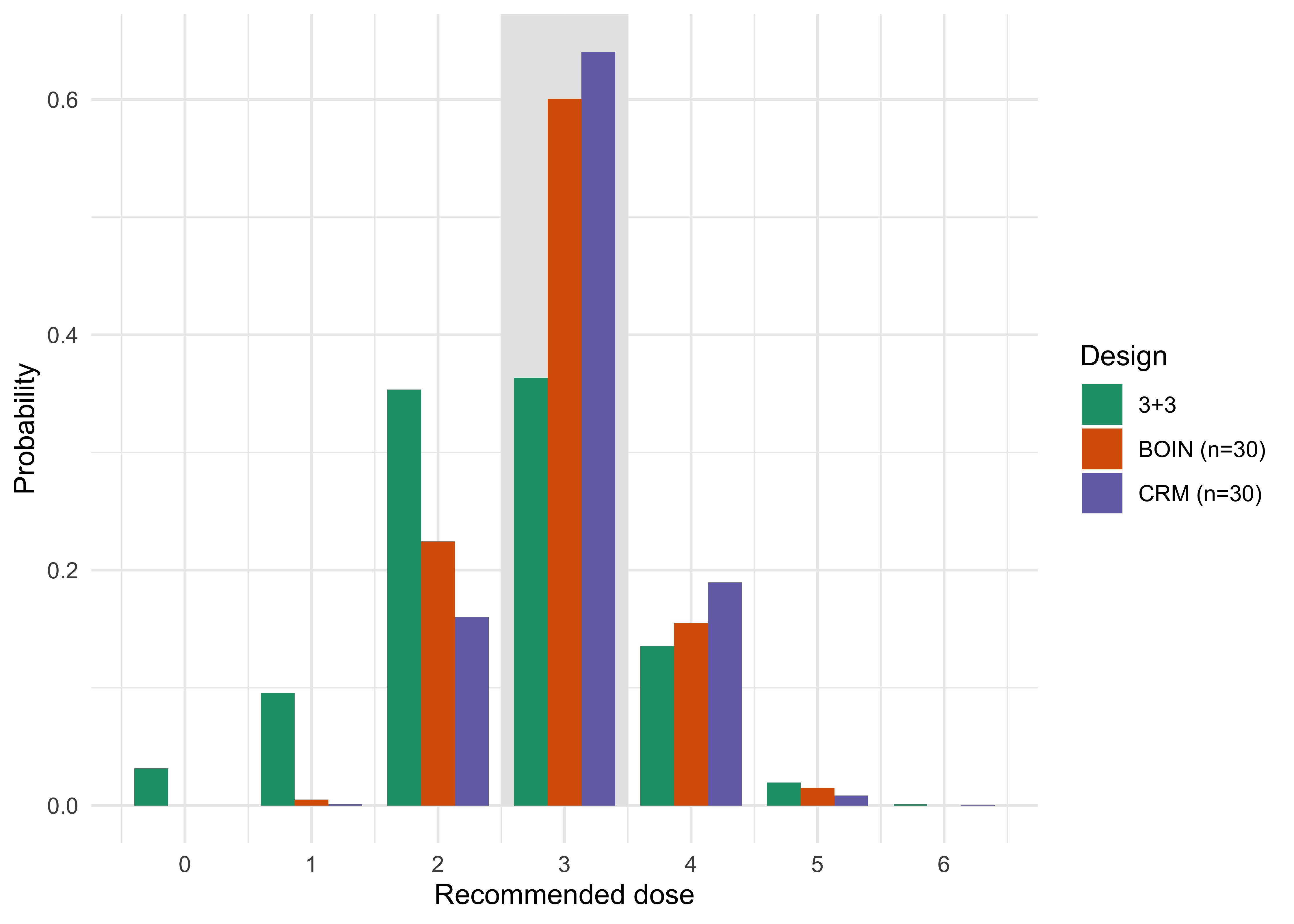
Two things stand out. First, the 3+3 finds the true MTD in only about 36 to 41 percent of trials across the three scenarios, and in roughly half of trials it recommends a dose below the MTD (for example 47 percent in scenario A, 53 percent in scenario B). The rule is conservative by construction: it stops as soon as a cohort of six shows two DLTs, and two DLTs in six is far from impossible at doses whose true DLT rate is well below the target. Second, its mean sample size is small, between about 10 and 19 patients. That is its virtue and its limitation: few patients are exposed at toxic doses (about three or fewer, on average, in every scenario), and little information is gathered at the recommended dose.

Figure 17.1 shows the distribution of the selected dose in scenario A for the three designs.

Show the R code
d <- do.call(rbind, lapply(names(designs), function(n)
  data.frame(Design = n, Dose = 0:6, Prob = dose_simulate(designs[[n]], S$A, 2000, 2)$sel)))
ggplot(d, aes(Dose, Prob, fill = Design)) +
  annotate("rect", xmin = 2.5, xmax = 3.5, ymin = 0, ymax = Inf, fill = "grey90") +
  geom_col(position = "dodge", width = 0.8) + scale_x_continuous(breaks = 0:6) +
  scale_fill_brewer(palette = "Dark2") + labs(x = "Recommended dose", y = "Probability") + theme_minimal()
Figure 17.1: Distribution of the dose recommended as the MTD in scenario A (true MTD is dose 3, shaded). 0 means no dose was judged tolerable.

What six patients can tell you

Most of the cost of the 3+3 is not in the rule but in the information it leaves behind. A trial that ends with one DLT in six patients at the recommended dose is described in the protocol as showing a “tolerable” dose. The thinness of what a 3+3 trial learns has been shown by exact enumeration of the rule (Reiner, Paoletti, and O’Quigley 1999; Y. Lin and Shih 2001) and in comparison with the CRM (Iasonos et al. 2008), and is discussed in our working paper (Polson and Sokolov 2026b); the arithmetic below is a Bayesian version of the same point. Take the prior on the DLT probability to be Beta(0.25, 0.75) (a weakly informative prior with prior mean 0.25 and the weight of one prior patient). One DLT in six patients gives a Beta(1.25, 5.75) posterior.

Show the R code
a <- 0.25 + 1; b <- 0.75 + 5
ci <- qbeta(c(0.025, 0.975), a, b)
post <- c(`Posterior mean` = a / (a + b), `Lower 95%` = ci[1], `Upper 95%` = ci[2],
  `P(DLT rate > 0.33)` = pbeta(0.33, a, b, lower.tail = FALSE))
knitr::kable(data.frame(Quantity = names(post), Value = round(post, 3)), row.names = FALSE)
Quantity Value
Posterior mean 0.179
Lower 95% 0.010
Upper 95% 0.511
P(DLT rate > 0.33) 0.141

The 95 percent posterior interval runs from 0.01 to 0.51. The same trial that is reported as having “found” a dose with a one-in-six observed DLT rate is compatible, at that level, with a DLT rate that is half. A frequentist exact (Clopper-Pearson) interval for one in six is wider still (roughly 0.004 to 0.64), so the problem is the sample size and not the Bayesian treatment of it. The designs below do not repair this by magic. They do three things: they use every patient treated at every dose (the 3+3 forgets all previous doses when it moves), they state the target toxicity rate, and they let the sample size be chosen deliberately instead of by the stopping rule.

What stays the same

A fair summary of the 3+3: it is simple, transparent and safe in the sense that few patients are exposed to high doses, at the price of a low chance of finding the MTD and a poor estimate of the DLT rate at the dose it recommends. For a trial of a drug with a well-understood toxicity profile and a small number of doses, a team may reasonably choose it. Simulation makes the consequences of choosing the 3+3 explicit and supports the design justification, because the simulation above is exactly the evidence on which it should be judged.

17.2 The Bayesian version: model-based and model-assisted designs

Chapter 6 updated a belief about a probability with data. A dose-finding design is that same update, repeated after every cohort and used to choose the next dose. The Bayesian designs differ from the 3+3 in two ways. They name a target toxicity rate \(\Gamma\). And they assume that the DLT probability increases with dose, so information at one dose informs the neighboring ones. They differ from one another in how much of that structure they use.

The continual reassessment method

The continual reassessment method (CRM) of O’Quigley, Pepe and Fisher (O’Quigley, Pepe, and Fisher 1990) was the first Bayesian design in phase 1 and remains the reference model-based design. In its simplest form it posits a one-parameter curve through \(K\) doses, \[ p_d(a) = \pi_d^{\exp(a)}, \qquad d = 1, \dots, K, \] where \(\pi_1 < \dots < \pi_K\) is a prespecified skeleton (a set of guessed DLT probabilities, one per dose) and \(a\) is an unknown parameter with a prior, here \(a \sim N(0, 1.34)\). After each cohort, the posterior of \(a\) is computed from the data at all doses, and the next cohort is given the dose whose posterior mean DLT probability is closest to \(\Gamma\). Two safety rules are standard: no skipping a dose when escalating, and a stopping rule if the lowest dose is judged too toxic. The original proposal treats one patient at a time; the version in use adds cohorts, no skipping of untried doses and a start at the lowest dose (Goodman, Zahurak, and Piantadosi 1995). The likelihood version (O’Quigley and Shen 1996) and the book of Cheung (2011) popularized the power working model used here, and Garrett-Mayer (2006) is a tutorial.

The consequence for the protocol is that the sponsor now writes down a skeleton and a prior, which the 3+3 never needed. The skeleton is not the truth; it is a shape. The design uses the data to move the whole curve up or down. In our simulation the skeleton (0.05, 0.12, 0.25, 0.40, 0.55, 0.70) is close to the truth in scenario A (it differs only at dose 2) and wrong in scenarios B and C; a real simulation report should include scenarios in which the skeleton is badly wrong.

With \(y_d\) DLTs among \(n_d\) patients at dose \(d\), the likelihood of \(a\) is \(\prod_d p_d(a)^{y_d}\{1-p_d(a)\}^{n_d - y_d}\). The posterior \(\pi(a \mid y) \propto \pi(a) \prod_d p_d(a)^{y_d}\{1-p_d(a)\}^{n_d-y_d}\) is one-dimensional, so it is computed on a grid of a few hundred points (as dose_crm() does) and the posterior mean of each \(p_d(a)\) is a weighted sum over the grid. No MCMC is needed. The one-parameter form is deliberately rigid: it is well-behaved with few patients because it cannot fit anything but a monotone curve. Richer two-parameter logistic models, such as the Bayesian logistic regression model used with escalation with overdose control (Neuenschwander, Branson, and Gsponer 2008), estimate the slope too and need informative priors to behave.

The chapter’s code uses dose_crm() from the book’s package bayestrials, which is written for teaching and for the simulations here. For production work the maintained CRAN packages are the tools to use: dfcrm and trialr for CRM and related Bayesian designs, and BOIN for the Bayesian optimal interval designs below (the boundaries computed by dose_boin_bounds() agree with BOIN::get.boundary). A sponsor’s statistical analysis plan should name the software and version that generated the simulation report.

The Bayesian optimal interval design

The Bayesian optimal interval (BOIN) design of Liu and Yuan (Liu and Yuan 2015) is a model-assisted design. It is derived from a Bayesian argument, but at the bedside it is a table. For each dose, the observed DLT rate \(\hat p_d = y_d/n_d\) is compared with two fixed boundaries. If \(\hat p_d \le \lambda_e\), escalate; if \(\hat p_d \ge \lambda_d\), de-escalate; otherwise stay. The boundaries are chosen to minimize the probability of a wrong decision between three simple hypotheses: the dose is at the target, it is below the target toxicity rate, at \(0.6\,\Gamma\), or it is overly toxic at \(1.4\,\Gamma\). The boundaries do not depend on the dose or on the number of patients treated.

Show the R code
bd <- dose_boin_bounds(0.25)
n <- c(3, 6, 9)
knitr::kable(data.frame(Patients = n, `Escalate if DLTs at most` = floor(bd[["escalate"]] * n + 1e-9),
  `De-escalate if DLTs at least` = ceiling(bd[["deescalate"]] * n - 1e-9), check.names = FALSE), align = "ccc")
Patients Escalate if DLTs at most De-escalate if DLTs at least
3 0 1
6 1 2
9 1 3

With cohorts of three, this rule says escalate on zero DLTs and de-escalate on one or more, which is more cautious than the 3+3 in the first cohort. A dose is eliminated, together with all higher ones, if the posterior probability that its DLT rate exceeds \(\Gamma\) exceeds 0.95 (with a uniform prior and at least three patients treated). At the end, the MTD is chosen as the dose whose isotonically smoothed DLT rate is closest to \(\Gamma\). The smoothing follows the reference implementation (BOIN::select.mtd): isotonic regression with inverse posterior-variance weights, and, when two doses are equally close with rates below the target, the higher one.

The practical appeal is that the protocol contains the same kind of table as the 3+3: a grid of numbers of DLTs and numbers of patients. A clinician needs no software on the day. The statistician has the operating characteristics, by simulation, in the design report. The FDA’s Drug Development Tools Fit-for-Purpose Initiative lists the BOIN design for dose finding, with a determination issued on 10 December 2021 (U.S. Food and Drug Administration 2025). That is a statement about a context of use (phase 1 dose finding with a toxicity endpoint) and does not exempt a sponsor from providing simulations for its own trial. A practical overview for oncology trialists is in Yuan et al. (2016), and an extension to drug combinations in R. Lin and Yin (2017).

The other interval designs: mTPI, mTPI-2 and Keyboard

BOIN is not the only design whose decisions are printed as a table. The toxicity probability interval designs divide the DLT-rate axis into an underdosing interval, an equivalence interval around the target and an overdosing interval. The first version is Ji, Li, and Bekele (2007), and its modified form (mTPI) (Ji et al. 2010) computes the posterior probability mass of each interval divided by the interval’s width and moves toward the interval with the largest value. The mTPI-2 design (Guo et al. 2017) changes how the intervals are formed, in response to a weakness of mTPI that its authors frame as an Ockham’s razor problem. The Keyboard design (Yan, Mandrekar, and Yuan 2017) lays equal-width keys, each as wide as the target interval, over the DLT-rate axis, and recommends the move toward the key with the highest posterior probability. As with BOIN, the protocol carries a table of decisions by number of DLTs and number treated, and the logic can be checked by hand.

Which to choose is an empirical question, and the evidence is simulation. Horton, Wages, and Conaway (2017) compared the CRM, mTPI and BOIN on the percentage of correct selection of the true MTD, patient allocation near it and an accuracy index, and Zhou, Yuan, and Nie (2018) compared several newer phase 1 designs on accuracy, safety and reliability. Those are comparisons in stated scenarios at stated sample sizes, like the comparison of this chapter, and the lesson is the same as for CRM and BOIN: the protocol should report the chosen design’s own operating characteristics in scenarios that include a badly placed target.

Comparing the designs

Back to Table 17.2. With 30 patients in cohorts of three, CRM selects the true MTD in about 52 to 71 percent of trials and BOIN in about 52 to 69 percent, against 36 to 41 percent for the 3+3. CRM and BOIN also make fewer under-selection errors, which is where the 3+3 loses most. But the table is honest in the other direction too. CRM and BOIN treat 30 patients, the 3+3 about 10 to 19. They therefore treat more patients at toxic doses in absolute terms (about 5 to 6 for CRM and BOIN against about 3 for the 3+3 in scenarios A and C) and see more DLTs. (Section 17.8 reports how rarely model-based designs have been used, and what happened when published 3+3 trials were re-run with them.)

Show the R code
small <- list("3+3" = dose_three_plus_three, "CRM (n=15)" = function(p) dose_crm(p, N = 15),
              "BOIN (n=15)" = function(p) dose_boin(p, N = 15))
g <- expand.grid(Design = names(small), Scen. = c("A", "B"), stringsAsFactors = FALSE)
r <- Map(function(d, s) dose_simulate(small[[d]], S[[s]], 2000, 1), g$Design, g$Scen.)
g$`P(correct MTD)` <- sapply(r, `[[`, "p_correct"); g$`Mean n` <- sapply(r, `[[`, "n")
g$`n toxic` <- sapply(r, `[[`, "n_toxic"); g$`Mean DLTs` <- sapply(r, `[[`, "dlts")
knitr::kable(g[order(g$Scen.), c(2, 1, 3:6)], row.names = FALSE, digits = 2)
sm <- function(d, s) sprintf("%.0f", 100 * g$`P(correct MTD)`[g$Design == d & g$Scen. == s])
Table 17.3: CRM and BOIN at a small sample size (n = 15, cohorts of 3), compared with the 3+3, scenarios A and B, 2,000 simulated trials per cell.
Scen. Design P(correct MTD) Mean n n toxic Mean DLTs
A 3+3 0.38 13.82 2.98 2.80
A CRM (n=15) 0.51 15.00 1.68 2.53
A BOIN (n=15) 0.46 15.00 1.11 2.25
B 3+3 0.36 18.98 2.03 2.71
B CRM (n=15) 0.28 15.00 0.00 1.25
B BOIN (n=15) 0.35 15.00 0.00 1.18

The comparison is not like for like, since a model-based design spends more patients to find the dose more reliably. Cutting the sample size to 15 (Table 17.3), a size comparable with the 3+3, the probability of selecting the MTD falls in scenario A to about 51 percent for CRM and 46 percent for BOIN (and in scenario B to 28 and 35 percent), against 38 and 36 percent for the 3+3. Both are then better than the 3+3 in scenario A. In scenario B CRM is worse and BOIN about level with the 3+3, with fewer patients at toxic doses in both. The result is a design-time choice that the protocol should make explicitly: how many patients is the MTD worth?

These are results for particular scenarios, a particular skeleton, a particular prior and a particular cohort size. They do not rank the designs in general, and the literature shows both CRM and BOIN performing well when properly calibrated. The point for the protocol is that a design can be judged only by running it, and that the simulation must include scenarios in which the skeleton is wrong, the MTD is at the top or bottom of the range, and every dose is too toxic.

Escalation with overdose control

Escalation with overdose control (EWOC) (Babb, Rogatko, and Zacks 1998) changes the criterion for the next dose. Instead of the dose whose estimated DLT rate is closest to \(\Gamma\), EWOC chooses the highest dose for which the posterior probability of overdosing (exceeding the MTD) does not exceed a feasibility bound \(\eta\) (several doses may satisfy the constraint), often starting at 0.25 and raised as the trial proceeds. A dose that has some chance of being too toxic is therefore not the one most likely to be chosen. This builds a patient-safety constraint into the decision itself, which is one reason EWOC was an early attempt to give ethical control a formal expression. The Bayesian logistic regression model (BLRM) of Neuenschwander, Branson, and Gsponer (2008) applies the same overdose-control idea to interval probabilities of the DLT rate under a two-parameter logistic model with informative priors, and with either design the dose-escalation decisions then rest on a posterior that depends strongly on the prior, which the FDA draft on Bayesian methodology says should be justified and subjected to sensitivity analysis (see Chapter 8).

A worked escalation decision with the logistic model

To see what the posterior looks like at a decision point, take doses of 1, 2, 4, 8 and 16 mg with reference dose 8 mg, and the two-parameter logistic model \(\mathrm{logit}\,p(d) = \log\alpha + \beta \log(d/8)\) with \(\beta = e^{\log\beta}\). The prior is \(\log\alpha \sim N(\mathrm{logit}\,0.25, 2^2)\), which centers the toxicity rate at the reference dose on the target of 0.25 with wide uncertainty, and \(\log\beta \sim N(0, 1)\). Four cohorts have been treated: 0 of 3 DLTs at 1 mg, 0 of 3 at 2 mg, 1 of 3 at 4 mg and 1 of 6 at 8 mg. Each dose is classified by its true DLT rate: underdosing below 0.16, target from 0.16 to 0.33, overdosing at 0.33 or above. Table 17.4 gives the posterior probability of each interval, computed on a grid.

Show the R code
B <- dose_blrm_table()
knitr::kable(data.frame(`Dose (mg)` = B$dose, `Mean DLT rate` = B$mean_tox, Under = B$p_under, Target = B$p_target, Over = B$p_over, Admissible = ifelse(B$admissible, "yes", "no"), check.names = FALSE), digits = c(0, 3, 2, 2, 2, 0))
Table 17.4: Posterior mean DLT rate and posterior probability that the DLT rate lies in the underdosing (below 0.16), target (0.16 to 0.33) or overdosing (0.33 or above) interval, after four cohorts. A dose is admissible if the probability of overdosing is at most 0.25.
Dose (mg) Mean DLT rate Under Target Over Admissible
1 0.049 0.95 0.05 0.00 yes
2 0.074 0.90 0.10 0.00 yes
4 0.123 0.73 0.25 0.02 yes
8 0.223 0.36 0.45 0.19 yes
16 0.375 0.17 0.32 0.51 no

The 16 mg dose is excluded, since its probability of overdosing is 0.51, above the bound of 0.25. Among the admissible doses, 8 mg has the highest probability of lying in the target interval (0.45, with 0.36 under and 0.19 over), so the next cohort receives 8 mg. The single DLT at 4 mg did not stop escalation: the model weighs it against the absence of toxicity at the lower doses and one in six at 8 mg, which is the use of all the data that the 3+3 rule forgoes. The result depends on the prior, as the text above says: rerun the table with a different prior_sd before trusting it.

Protocol language

TipIn the protocol: a model-based dose-escalation design

State the target toxicity rate \(\Gamma\) and the DLT definition and window. State the dose ladder, the starting dose, the cohort size and the maximum sample size. For CRM, give the skeleton and the prior on its parameter, with the reason for each. For BOIN, give the escalation and de-escalation boundaries and the elimination rule. State the no-skipping rule and the stopping rule for an overly toxic lowest dose. Attach a simulation report with at least five scenarios (including a flat-toxic scenario and one where the MTD is the top dose) with the probability of correct selection, the probability of overdose selection, the number of patients at doses above the target, and the sensitivity of each to the skeleton or prior. Specify who can override the design’s recommendation (usually a safety review committee) and in what circumstances, for example when late toxicities, or toxicities after the DLT window, appear. See Chapter 23 for the general protocol table.

17.3 Beyond the MTD: efficacy, toxicity and dose optimization

Why the MTD is a poor target for modern agents

The MTD paradigm assumes that more is better until it hurts. That was a reasonable working belief for cytotoxic chemotherapy, and it was written into the designs above, which look only at toxicity. It is a poor assumption for targeted therapies, immunotherapies and antibody-drug conjugates. For such agents the dose-response curve for efficacy may reach a plateau well below the MTD, a drug may be taken for months or years rather than for a few cycles, and chronic low-grade toxicity may lead to dose reductions and discontinuations that cannot be seen in a short DLT window. A dose chosen as the MTD can then be both more toxic and no more effective than a lower one. The FDA’s stated concern is that choosing the dose this way can leave patients on doses with more toxicity and no more benefit than a lower dose (U.S. Food and Drug Administration 2024). The rationale for the initiative is set out by FDA authors in Shah et al. (2021), and the statistical principles, with a review of FDA initial approvals of small molecules and antibody-drug conjugates in 2019 to 2021, in Fourie Zirkelbach et al. (2022).

What the FDA guidance asks

The final guidance of August 2024 (docket FDA-2022-D-2827, Oncology Center of Excellence with CDER and CBER) has a stated scope. The guidance does not address first-in-human starting-dose selection. It does not specifically address dosage optimization for radiopharmaceuticals, cellular and gene therapies, oncolytic viruses, microbiota or cancer vaccines, or pediatric development, although some recommendations may apply to these settings. Developed through Project Optimus, launched in 2021 (U.S. Food and Drug Administration 2021, 2024), the guidance recommends that sponsors of oncology products take a dose selection approach different from that of the 3+3. In paraphrase, and the guidance should be consulted for the precise wording, it recommends the following.

  • Doses to be taken to registrational trials should be chosen on a broader basis than the MTD alone: pharmacokinetics, pharmacodynamics, exposure-response for efficacy and safety, and clinical safety, tolerability and activity, including late and low-grade toxicities.
  • Dose-ranging in the clinic should compare several dosages, and where feasible with randomization, rather than rely on a single-arm escalation to one dose. The comparison is intended to characterize the dose-response and dose-toxicity relationships, not to establish superiority or noninferiority of one dose over another at registrational error rates.
  • Model-based and model-informed methods, including Bayesian ones, are expected to be useful in this process, and sponsors should discuss the design with FDA early. The guidance does not require a specific design, and neither does it exclude the 3+3.
  • Dose selection should be explained in the context of the intended population and the treatment’s schedule.

ICH E4 (U.S. Food and Drug Administration 1994) already established these principles: the dose-response relationship should be characterized during development, several dose-response designs (including Bayesian and pharmacometric methods) are discussed, prospective randomized multidose studies are recommended, and the highest tolerated dose need not be optimal even in life-threatening disease. The August 2024 guidance gives them a focused application to contemporary oncology dosage optimization. For the exposure-response models that support the choice, ICH M15 (International Council for Harmonisation 2026) is the framework. A sponsor who uses a model to select between two doses has to state the question of interest and the context of use, and assess how much weight the model carries in the decision and how costly a wrong decision would be.

A Bayesian formulation: utility

A Bayesian can state the dose problem directly. Let \(\pi_E(x)\) be the probability of a favorable efficacy outcome at dose \(x\) and \(\pi_T(x)\) the probability of a toxicity. Elicit a utility for each of the four joint outcomes, as in the utility-based designs described in our working paper (Polson and Sokolov 2026a): efficacy without toxicity is the best, no efficacy and toxicity the worst, with efficacy and toxicity together somewhere in between. The expected utility of a dose is the average of these utilities under the posterior. A design chooses the dose that maximizes it, among those that are acceptable: meeting a minimum efficacy and a maximum toxicity bound at a stated posterior probability.

Show the R code
x <- 1:6; pE <- plogis(-2.5 + 1.6 * (x - 1) - 0.2 * (x - 1)^2); pT <- S$B
u <- 100 * pE * (1 - pT) + 40 * pE * pT - 60 * (1 - pE) * pT
d <- data.frame(Dose = x, Panel = rep(c("Probability", "Expected utility"), c(12, 6)),
  Series = c(rep(c("efficacy", "toxicity"), each = 6), rep("utility", 6)), Value = c(pE, pT, u))
ggplot(d, aes(Dose, Value, colour = Series, linetype = Series)) + geom_line() + geom_point() +
  geom_vline(data = data.frame(Panel = "Expected utility", x = which.max(u)), aes(xintercept = x), linetype = 3) +
  facet_wrap(~ Panel, scales = "free_y") + scale_colour_brewer(palette = "Dark2") + theme_minimal() +
  labs(x = "Dose level", y = NULL)
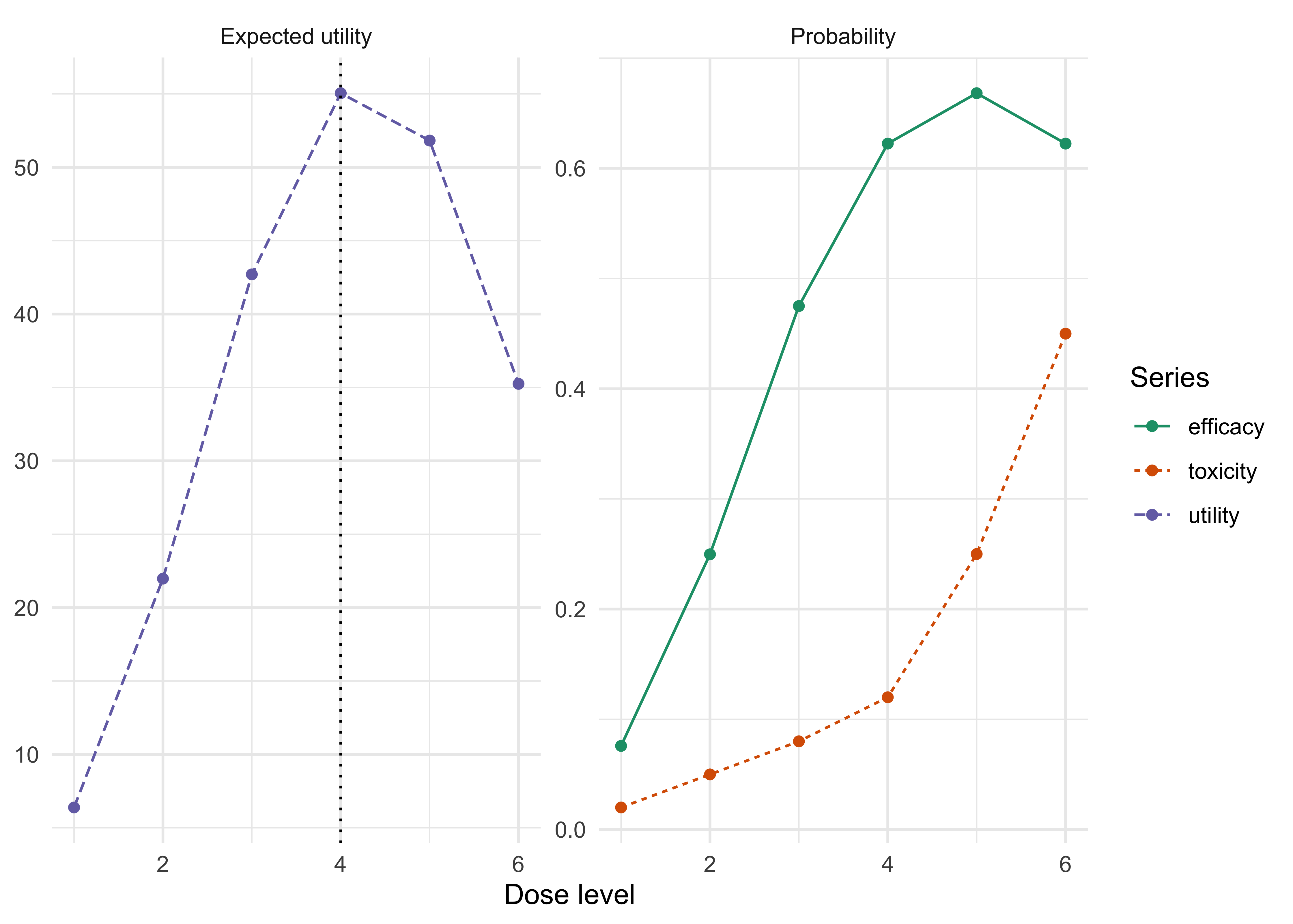
Figure 17.2: Illustrative true curves. Toxicity (scenario B) reaches 0.25 at dose 5, so the MTD is dose 5. Efficacy is non-monotone and plateaus at dose 4 to 5. The dose that maximizes expected utility is dose 4, below the MTD.

In Figure 17.2 the dose with the largest expected utility is dose 4, one level below the MTD, because the efficacy gain from dose 4 to dose 5 is small and the toxicity cost is not. The utilities are the price of the method. They are an elicited, subjective choice, and the dose that wins depends on them. The protocol should record who elicited them, from whom, on what basis, and how the result changes if they change (see the sensitivity analysis in Chapter 8 for the same point about priors). The numbers 100, 40, 0 and -60 above are illustrative, not clinical.

EffTox and phase 1/2 designs

The EffTox design of Thall and Cook (Thall and Cook 2004) formalizes this. It models efficacy and toxicity probabilities as functions of dose, with a quadratic logistic form for efficacy so that the dose-efficacy curve can turn down, a monotone logistic form for toxicity, and a copula for the association between the two outcomes in the same patient (Polson and Sokolov 2026a). Rather than ask for utilities for four outcomes, the original EffTox design elicits a trade-off contour in the plane of \((\pi_T, \pi_E)\): the investigator names several pairs of efficacy and toxicity probabilities that are equally desirable. A dose is acceptable if its posterior probabilities satisfy the minimum efficacy and maximum toxicity constraints, and the next cohort receives the acceptable dose with the highest desirability. Early phase 1/2 designs of this kind are described in Thall and Russell (1998). Later work extends the utility approach to ordinal efficacy and toxicity outcomes and combinations of agents, including the utility-based combination design of Houede and colleagues (Houédé et al. 2010) and an adaptive-randomization version for bivariate ordinal outcomes (Thall et al. 2015). Book-length treatments are Yuan, Nguyen, and Thall (2016) and Thall (2024).

Three things are different from the toxicity-only designs. The trial needs a probabilistic model for efficacy, so it needs an efficacy endpoint that can be observed quickly enough to be used during the trial (a response, a biomarker, a PD measure). Early efficacy readouts that are only surrogate for the clinical endpoint bring a surrogacy question into the dose decision. The designs need larger samples, usually 40 to a few hundred. And the elicitation of the contour or utility is an extra step that must be defended. In return the trial can state what it says about the dose-response, and the dose that it picks is accompanied by a distribution of efficacy and toxicity at that dose.

Late-onset toxicity and utility-based interval designs

The phase 1/2 designs above need the outcome of each cohort before the next one is dosed, which is the logistic problem of late-onset toxicity. The time-to-event CRM of Cheung and Chappell (2000) incorporates incomplete follow-up from patients without an observed DLT, commonly using the fraction of the observation window completed, while observed DLTs contribute full event information, so that enrollment need not pause while earlier patients are followed. Yuan et al. (2018) built the same idea into the interval design: TITE-BOIN allows real-time dose assignment for new patients while some enrolled patients’ toxicity data are still pending, and so addresses both late-onset toxicity, which is common for targeted agents and immunotherapy, and rapid accrual. For the efficacy-toxicity trade-off, BOIN12 of R. Lin et al. (2020) targets the optimal biologic dose that optimizes the risk-benefit trade-off, for agents whose efficacy does not necessarily increase with dose, and is built to be simple enough that its decision rules can be tabulated in the protocol as BOIN’s are. In the setting of Figure 17.2, where efficacy plateaus below the MTD, for the illustrative true curves the MTD is dose 5 and expected utility is highest at dose 4. Yuan, Zhou, and Liu (2024) review the design strategies for dose-optimization trials and the practical considerations in planning them, including the randomized comparison the FDA guidance recommends.

Randomized dose comparison, and what a regulator will ask

The guidance recommends comparing dosages directly, and a randomized comparison of two or three candidate doses after the escalation phase is the common implementation. The trial need not be powered for formal superiority or noninferiority between doses at registrational error rates. Its size should support sufficiently precise assessments of safety and antitumor activity at each dosage, and the doses are not expected to differ by much in efficacy, which is why the evidence is expected to include PK/PD, safety and tolerability, and modeling. A Bayesian formulation is to compute the posterior probability that each dose’s efficacy is within a prespecified margin of the best dose and the posterior probability that its tolerability is better, and to select the lowest dose that meets both, with simulated operating characteristics. The chapter on simulation (Chapter 14) describes the report. For a design of this kind a reviewer is likely to ask the following.

  1. What are the operating characteristics for choosing a dose that is not the one that maximizes efficacy: the probability of selecting a dose that is too low or too toxic under each scenario?
  2. How were the utility, trade-off contour or margins elicited, and what changes if they are altered?
  3. What priors were used for the efficacy and toxicity models, and how much do they affect the dose choice?
  4. How are late toxicities and dose reductions after cycle 1 handled in the dose decision?
  5. What is the role of the exposure-response model (Section 17.3) and how was its risk assessed under M15?

17.4 Dose-response estimation outside oncology: MCP-Mod

Most of this chapter concerns oncology, where the dose question is how much toxicity to accept. Most other programs run a phase 2 dose-ranging study whose question is the shape of the dose-response curve and which dose to take to phase 3. The traditional method that regulators know best here is MCP-Mod, which combines a multiple comparison step with a modeling step (Bretz, Pinheiro, and Branson 2005; Pinheiro et al. 2014). It is on FDA’s fit-for-purpose list with a determination of 26 May 2016 (U.S. Food and Drug Administration 2025), and it is the dose-finding method on that list that belongs to the frequentist tradition.

The method has two steps. First, before the data, the protocol names a candidate set of dose-response shapes (for example linear, Emax, exponential and umbrella) with guessed parameters, and from each shape computes the contrast of the dose means that has the most power if that shape is true. The test of “no dose-response” is the maximum of these contrast statistics, and its critical value comes from their joint (multivariate normal or \(t\)) distribution, so the familywise type I error over the candidate shapes is held at one-sided 0.025 when there is no dose-response at all. Second, if the test finds a signal, the models that passed are fitted, and the dose-response curve and a target dose (for example the smallest dose with a clinically relevant effect) are estimated, by selecting a model or by averaging. The chunk below shows the first step for five doses and 40 patients per dose with a known standard deviation of 1 and candidate shapes that never fall below placebo, and compares it with two traditional analyses of the same data: the top dose against placebo, and the best of four pairwise comparisons with a Bonferroni correction.

Show the R code
doses <- c(0, 10, 25, 50, 100); n <- 40
shapes <- cbind(linear = doses / 100, emax = doses / (doses + 15), exponential = (exp(doses / 50) - 1) / (exp(2) - 1),
                umbrella = 1 - (doses / 50 - 1)^2)          # candidate shapes, none below placebo
mcp <- mcp_contrasts(shapes)                                 # optimal contrasts and the critical value
truth <- list(Flat = rep(0, 5), `Emax with plateau` = 0.5 * doses / (doses + 10), Linear = 0.5 * doses / 100,
              Umbrella = 0.5 * (1 - (doses / 50 - 1)^2), `Harmful, linear decline` = -0.5 * doses / 100)
mcp_tab <- t(sapply(truth, mcp_power, contrasts = mcp$contrasts, crit = mcp$crit, n = n, seed = 1))
knitr::kable(mcp_tab, digits = 3, col.names = c("MCP-Mod contrast test", "Top dose vs placebo", "Bonferroni, four doses"))
Table 17.5: Probability of a one-sided 0.025 dose-response signal under five true dose-response shapes (flat, an Emax shape with a plateau, a linear shape, an umbrella shape that returns to the placebo mean at the top dose, and a harmful linear decline) for the MCP-Mod multiple contrast test, the top dose against placebo, and the best of four Bonferroni-adjusted pairwise comparisons. Candidate shapes: linear, Emax, exponential and umbrella, all at or above placebo. Five doses, 40 patients per dose, standard deviation 1, 20,000 simulated trials per cell.
MCP-Mod contrast test Top dose vs placebo Bonferroni, four doses
Flat 0.024 0.025 0.022
Emax with plateau 0.523 0.527 0.493
Linear 0.617 0.609 0.424
Umbrella 0.686 0.025 0.471
Harmful, linear decline 0.015 0.000 0.004

With four candidate shapes the critical value of the maximum contrast statistic is 2.37, against 1.96 for one test and 2.50 for a Bonferroni correction over four comparisons, because the contrasts are positively correlated for the monotone shapes. The type I error is held at the flat truth (0.024), which is where the familywise guarantee applies, and the power of the contrast test is similar to the best traditional test when the true shape is monotone (Table 17.5). Its advantage is visible when the true curve is not monotone: when the top dose returns to the placebo mean the top-dose comparison has only its type I error rate (0.025), the Bonferroni comparison has 0.47, and the contrast test with an umbrella among the candidates has 0.69. The test detects a non-flat dose-response in the directions of the candidates, not benefit at some dose. A declining truth can still trigger a contrast when the candidates allow declines, which is why the candidates are chosen as benefit shapes (Bretz, Pinheiro, and Branson 2005); with the candidates here a harmful linear decline signals in only 0.015 of trials. The price is that the candidate set is a pre-specified list, and a truth outside it loses power; this is the dose-response counterpart of the skeleton choice for the CRM.

The Bayesian designs in this chapter allocate and decide adaptively: ASTIN (Grieve and Krams 2005; Krams et al. 2003) and the Bayesian dose selection in the lecanemab and AWARD-5 examples (Section 17.8). The operating characteristics of MCP-Mod, like those of any other design, are found by simulation in the scenarios the protocol names.

17.5 Adaptive enrichment and subgroup-specific doses

When benefit, or the best dose, differs by a biomarker-defined subgroup, broad enrollment can dilute the effect estimates, and a single dose may be wrong for part of the population. An enrichment design starts with broad enrollment and restricts to responsive subgroups as data accumulate (Polson and Sokolov 2026a). At each interim analysis, subgroup-specific posterior probabilities of benefit, \(\Pr(\theta_g > 0 \mid \text{data})\) for subgroup \(g\), map to one of three actions: continue broadly, restrict enrollment to the promising subgroups, or stop. The thresholds that govern these actions are calibrated by simulation, which is exactly the procedure the FDA draft Bayesian guidance asks for (U.S. Food and Drug Administration 2026). The multiplicity cost is real: subgroup-by-interim looks multiply the number of opportunities for a chance finding, and Chapter 10 describes the shrinkage and error-control tools that apply. Hierarchical models that borrow strength across subgroups (Chapter 19) are the Bayesian answer to the same problem. For a dose-finding trial the usual practice is to treat the dose-selection and the enrichment decisions separately unless the trial is built for both.

17.6 Seamless designs: carrying the dose decision forward

Phase 2/3

A conventional program has a phase 2 dose-finding trial, a gap in which the sponsor analyzes the data, writes a new protocol and opens new sites, and a phase 3 trial. A seamless phase 2/3 design merges the two. A first stage compares several doses or regimens with a control and selects one or two on interim data, and a second stage continues into confirmation under a prespecified rule. The statistical machinery is older than the guidance: Thall, Simon, and Ellenberg (1988) proposed two-stage designs that select among treatments and then test, Stallard and Todd (2003) gave sequential phase III designs that select the most promising treatment at the first interim analysis, and Bretz et al. (2009) review confirmatory adaptive designs, including combined phase II/III studies with treatment selection at an interim. The common structure is selection at the interim followed by a pre-specified final test that accounts for the selection. In an inferentially seamless design, data from the first stage for the selected dose are used in the final test, so the analysis has to account for the fact that the dose was selected because it looked good. In an operationally seamless design, the stages run under a single protocol but the final analysis uses second-stage data only. The motivation is the elimination of the “dead time” between phases, and the use of the trial’s own data to choose a dose rather than committing to a weak one. The price is complexity in the design, a need for a pre-specified selection rule, and the inferential adjustment. FDA’s adaptive design guidance (U.S. Food and Drug Administration 2019) expects the selection rule, the control of the type I error probability, and the firewall that protects the unblinded interim data to be written down in advance, and treats seamless designs under the same principles as other adaptive designs.

A simulation study of the inferentially seamless case in which one arm is selected at the end of the first stage found that pooling the two stages and using an adjusted final alpha, as in a group sequential design, does better than analyzing the second stage alone at full alpha, and slightly better than a combination test. It also found that putting roughly 30 to 50 percent of the patients in the first stage is close to optimal across a range of dose-response shapes (L. R. Berry et al. 2024). Two cautions apply to sizing. The power calculated for the arm that is eventually selected overstates the power of the design, because the first stage sometimes advances the wrong arm, so the true power must be found by simulating the selection. And when the first-stage endpoint is delayed, the patients enrolled while it matures belong to the cost of the first stage and the planned split should count them.

The two best-documented cases of Bayesian dose finding that continues into later stages, dulaglutide (AWARD-5) and lecanemab, are described in Section 17.8.

17.7 Side by side: what changes in the protocol

3+3 CRM / BOIN (toxicity-only) EffTox, utility, randomized dose comparison
Target None stated (implies a DLT rate near 0.2 or below) Target DLT rate \(\Gamma\) Dose with best benefit-risk trade-off, subject to acceptability bounds
Uses data from other doses No Yes (model, or isotonic smoothing) Yes
What goes in the protocol The rule Target, skeleton and prior (CRM) or boundaries (BOIN), cohort size, maximum n, stopping rules Models for efficacy and toxicity, priors, utilities or contour, acceptability bounds, selection rule
Typical n 10 to 25 (rule-determined) 20 to 40, fixed 40 to a few hundred
Evidence the regulator expects Rationale for the DLT definition and doses Simulated operating characteristics in several scenarios Same, plus elicitation record, sensitivity to utilities and priors, PK/PD and exposure-response support
Where it is the better choice Familiar agent, few doses, no model support available Most phase 1 trials with a toxicity endpoint Targeted, immunotherapy and ADC agents where the MTD is not the target (see the FDA 2024 guidance)
Main risk Under-dosing, poor estimate at the recommended dose More patients, a model-dependent answer if the skeleton or prior is poor Utility elicitation, surrogate efficacy endpoint, larger sample

What stays the same is that a dose-escalation design is a decision rule fixed before the first patient and judged by its operating characteristics, and that safety oversight by a committee with the power to override stays in place for every design. What changes is that the rule can use all the data, that the question can be about the benefit-risk trade-off, and that the evidence offered to the regulator is a simulation report and a model assessment, not an appeal to convention.

17.8 In practice

How often are model-based designs used, and does it matter?

The 3+3 survives mostly out of habit. Model-based designs were used in 1.6 percent of phase 1 trials published from 1991 to 2006 and in 6.4 percent of those published from 2012 to 2014, according to the figures reported by Love et al. (2017) (who cite an earlier survey for them). Their review and survey of investigators named the barriers: a lack of training, investigators’ preference for the 3+3, and limited design resources available before a trial is funded. Rogatko et al. (2007) is the earlier paper that documented the gap between published methods and the designs that trials used. The other side of the record is reassuring on safety: a review of 53 completed phase 1 cancer trials published from 2003 to 2013 that used the CRM or a variant concluded that the model-guided escalation was safe and generalizable (Iasonos and O’Quigley 2014).

The most direct evidence of what the 3+3 costs is a re-analysis. Silva et al. (2021) sampled 60 published dose-finding trials, took the 22 that had used the 3+3, and re-applied the CRM and BOIN to the published data, at target toxicity rates of 0.25 and 0.30 and without the expansion cohorts. The model-based designs recommended a different dose from the published MTD in a number of trials, treated fewer patients at suboptimal doses and escalated faster. Lesson. The reanalysis shows that alternative designs can recommend different doses. Because the true MTDs were unknown and some outcomes were simulated, it does not establish their real-world correct-selection probabilities. The obstacle to adoption is not statistical but organizational, and a protocol that offers a one-page table (BOIN) removes part of it.

BOIN and FDA’s fit-for-purpose determination

The BOIN design of Liu and Yuan (2015) is the one model-assisted design for which FDA has issued a determination: the Drug Development Tools Fit-for-Purpose list records a determination for BOIN dose finding dated 10 December 2021 (U.S. Food and Drug Administration 2025). What was reviewed was the method for a stated context of use (phase 1 dose finding with a toxicity endpoint). Lesson. The regulator’s acceptance attaches to a method and a context of use, and a sponsor still has to supply its own simulations and a protocol-specific justification. Chapter 3 places the fit-for-purpose initiative among FDA’s other tools.

Sotorasib and the dose that was not optimized

Sotorasib, a KRAS G12C inhibitor for non-small-cell lung cancer, is the case most often cited for Project Optimus. The pivotal single-arm trial (Skoulidis et al. 2021) used the 960 mg dose, and the accelerated approval of May 2021 came with a postmarketing requirement to compare that dose with a lower one. The randomized comparison of 960 mg and 240 mg was run only after approval. Lesson. This is the situation the August 2024 guidance (U.S. Food and Drug Administration 2024) was written for: a dose chosen without a randomized comparison of lower doses, with the evidence for a lower dose collected only after approval. The cost of the dose question is then borne by patients and by a postmarketing study, rather than by a randomized comparison in phase 1/2.

Dulaglutide (AWARD-5): seamless dose finding

The best-documented example of a Bayesian seamless dose-finding design is the AWARD-5 trial of dulaglutide in type 2 diabetes, which started in 2008 with seven doses and two controls (Geiger et al. 2012; D. A. Berry 2025). Stage 1 used response-adaptive randomization with interim analyses every two weeks, scored by a composite clinical utility index combining HbA1c, weight, heart rate and blood pressure. Longitudinal modeling predicted the 12-month outcome from early data, so that doses could be chosen before anyone reached the primary endpoint. The algorithm selected two non-adjacent doses (0.75 and 1.50 mg) at the earliest permitted time and the trial moved to stage 2, fixed randomization against the controls. The dose-finding results are reported in Skrivanek et al. (2014), and the design in Geiger et al. (2012). The data monitoring board could depart from the algorithm only on safety, and did so: in April 2009 randomization to the 3.0 mg dose was stopped on its recommendation after increases in heart rate and concerns about pancreatic safety (European Medicines Agency 2014). Both doses were approved by FDA in 2014. By Berry’s estimate the seamless design saved at least a year compared with separate phase 2 and phase 3 trials (D. A. Berry 2025).

Lesson. This is a utility-based design in the sense of the previous section, and it shows the pattern of regulation that has to be in place: a prespecified algorithm, an agreed role for the DMC, and a simulated operating-characteristics report. A sponsor of such a design today would seek agreement with the regulator in advance, by the routes described in Chapter 3.

Lecanemab: Bayesian dose finding in phase 2b

Study 201 of lecanemab in early Alzheimer’s disease was a Bayesian phase 2b trial with five dose regimens and placebo, with response-adaptive allocation and interim analyses beginning after 196 patients and every 50 patients thereafter (Swanson et al. 2021; D. A. Berry 2025). It identified 10 mg/kg biweekly as the estimated 90 percent effective dose (the dose achieving 90 percent of the modeled maximum effect). The trial did not meet its prespecified 12-month primary success criterion: the posterior probability of at least a 25 percent reduction in decline was 0.64, short of the required 0.80 (D. A. Berry et al. 2023). The prespecified 18-month clinical and biomarker results were part of the broader evidence package, and the selected regimen was carried into the subsequent phase 3 program. Lesson. The case shows two things relevant to a dose-optimization protocol. A design can fail its primary criterion and still produce the right dose, which is why the protocol should say in advance how the dose-selection evidence will be read in that event. And a prespecified Bayesian criterion that is not met is a result, to be reported as one.

ASTIN: a Bayesian adaptive dose-response trial in stroke

NoteASTIN (Krams et al. 2003)

The Acute Stroke Therapy by Inhibition of Neutrophils (ASTIN) trial was a Bayesian adaptive dose-response study of a neutrophil inhibitor in acute ischemic stroke (Krams et al. 2003). Rather than assign patients to a few fixed doses, it modeled the dose-response curve over a wide dose range with a smoothing model, so that the response at each dose borrowed strength from its neighbors, and used the accumulating posterior to choose the doses of later patients, to target the dose giving close to the maximum effect, and to stop early for efficacy or futility under prespecified rules. The trial stopped for futility at an interim analysis. The design paper is Grieve and Krams (2005). The point for this chapter is that the dose-finding model, the allocation rule and the stopping rule were all specified in advance and evaluated by simulation, as the 2026 FDA draft expects for a Bayesian design. We keep the description general: the exact dynamic linear model and allocation criterion should be taken from the original papers, not from this summary.

TipTry it in the lab

The open simulator at https://nytel.ai/testing/14-studio.html lets you set doses, adaptive allocation and scenarios and read off operating characteristics tables. Before opening it, predict how a design that updates after every cohort should behave when the true dose-response is flat across the top two doses, then change the true curves in the scenarios of this chapter (dose_scenarios()) and check your prediction.

Key points

  • The 3+3 is simple and exposes few patients to toxic doses, but in our simulations it selects the true MTD in only about 36 to 41 percent of trials, and under-selection is its most common selection error in these scenarios. Its operating characteristics can be obtained by exact enumeration or simulation, and they should be reported.
  • One DLT in six patients with a Beta(0.25, 0.75) prior leaves a 95 percent posterior interval for the DLT probability of 0.01 to 0.51. Small phase 1 trials identify a dose much less precisely than their rule suggests (see Reiner, Paoletti, and O’Quigley (1999) and Polson and Sokolov (2026b)).
  • CRM and BOIN name a target toxicity rate and use the data from all doses. In our scenarios, with 30 patients, they select the true MTD more often than the 3+3, at the price of more patients, and a design must be compared at a stated sample size. BOIN is listed in FDA’s fit-for-purpose initiative (determination of 10 December 2021) for a defined context of use (U.S. Food and Drug Administration 2025).
  • The MTD is the wrong target for many modern agents. The August 2024 FDA guidance recommends choosing the dosage on pharmacokinetic, pharmacodynamic, safety and efficacy evidence, preferably with a randomized comparison of several dosages (U.S. Food and Drug Administration 2024).
  • Utility-based and EffTox designs make the benefit-risk trade-off explicit. The price is an elicited utility or contour, an efficacy model and endpoint, and a larger sample, all of which a regulator will ask about.
  • Seamless phase 2/3 designs remove the gap between dose selection and confirmation, and require a prespecified selection rule, type I error control that accounts for the selection, and simulated operating characteristics. The AWARD-5 trial (Section 17.8) is the documented precedent.
  • Exposure-response models that support a dose choice fall under ICH M15: state the context of use and assess model influence and the consequence of a wrong decision (International Council for Harmonisation 2026).
NoteDiscussion questions
  1. A sponsor proposes a 3+3 design for a first-in-human trial of a targeted agent with six doses and a target DLT rate of 0.25. Using the simulation in this chapter, what would you ask them to add to the protocol, and what would you accept as a reason to keep the 3+3?
  2. Table 17.2 shows the model-based designs treating more patients at toxic doses than the 3+3. Is that a defect of the designs, of the comparison, or both? How would you set the sample size for a CRM or BOIN trial?
  3. For an antibody-drug conjugate with a plateau in response above dose 3 of 6, and a rising rate of dose reductions, how would you use the 2024 FDA guidance to design the dose-selection stage? What would be the primary decision rule, and what would the simulation report show?
  4. A utility-based design selects a dose below the MTD. Who should provide the utilities, how should the trial record them, and what sensitivity analysis would convince a reviewer?
  5. In a seamless phase 2/3 design with 3 candidate doses, what are the arguments for and against letting the first-stage data count toward the final test?