Most confirmatory trials in cardiology and oncology are event driven. The primary endpoint is the time to death, progression or a major adverse cardiovascular event, the analysis is a log-rank test or a Cox model, and the trial ends not at a fixed sample size but when a target number of events has accrued. SELECT and REWIND (Chapter 21) are both of this kind: SELECT planned 1,225 events and observed 1,270, REWIND observed 1,257. A trial of 17,604 patients is, statistically, a trial of about 1,270 events.
The Bayesian treatment of these trials is simpler than its reputation. For the decisions that matter (whether to stop at an interim analysis, how confident to be in a hazard ratio, whether a promising interim justifies more events) almost everything follows from two facts: the information about a log hazard ratio is proportional to the number of events, and the information about a single hazard is a gamma posterior. The chapter starts with the traditional analysis (log-rank test, Cox model, Schoenfeld’s event formula), then works through both facts with numbers, then turns to the case that breaks the first fact, non-proportional hazards.
ImportantRegulatory anchor
No FDA or ICH document is devoted to the Bayesian analysis of time-to-event data, and, as far as we are aware, none is devoted to non-proportional hazards or to restricted mean survival time. The following documents set the frame; Chapter 3 gives each one’s status.
ICH E9(R1), Addendum on Estimands and Sensitivity Analysis (Step 4, November 2019) (International Council for Harmonisation 2019). For a time-to-event endpoint the estimand must name the population, the variable (time to first event, or a composite), the handling of intercurrent events such as treatment discontinuation, rescue therapy or death before the non-fatal event, and the summary measure. A hazard ratio is one summary measure; the difference in restricted mean survival time or in survival probability at a landmark time are others. The choice is made before the trial, not after the curves are seen.
ICH E9, Statistical Principles for Clinical Trials (1998) (International Council for Harmonisation 1998). Section 3.5 on sample size and section 4.5 on interim analysis apply unchanged to event-driven trials: the number of events, and the assumptions behind it, must be stated in the protocol, and the interim plan must be fixed in advance.
FDA, Use of Bayesian Methodology in Clinical Trials of Drug and Biological Products (draft guidance, January 2026) (U.S. Food and Drug Administration 2026). A draft, which recommends and does not require. Its success criteria are posterior probabilities of the form \(\Pr(\delta > a \mid \text{data}) > c\), and nothing in it is specific to time-to-event data. For a trial with a frequentist statistical analysis plan, the operating characteristics of a Bayesian rule on the hazard ratio are calibrated as in Chapter 14.
FDA, Clinical Trial Endpoints for the Approval of Cancer Drugs and Biologics (final guidance, December 2018) (U.S. Food and Drug Administration 2018). Discusses overall survival, progression-free survival and related endpoints and the biases of each. It is the document sponsors most often cite for oncology time-to-event endpoints; it does not prescribe a method for non-proportional hazards.
18.1 The traditional analysis
Let \(T\) be the event time and \(S(t) = \Pr(T > t)\) the survival function. The hazard is \(h(t) = \lim_{\delta \to 0}\Pr(t \le T < t + \delta \mid T \ge t)/\delta\), and the cumulative hazard is \(H(t) = \int_0^t h(u)\,du\), so that \(S(t) = e^{-H(t)}\). Patients still event-free at the data cutoff, or lost to follow-up, are censored: their event time is only known to exceed the last contact. The Kaplan-Meier estimate of \(S(t)\)(Kaplan and Meier 1958) handles censoring without a model, and it is the curve every trial report draws.
The treatment comparison has two standard forms. The log-rank test (Mantel 1966; Peto and Peto 1972) compares, at each event time, the observed number of events in the treated arm with the number expected if the two arms shared one hazard, and sums the differences. It is the score test of a proportional hazards model. The Cox model (Cox 1972) writes \(h(t \mid z) = h_0(t)e^{-\theta z}\) for a treatment indicator \(z\), leaves the baseline hazard \(h_0(t)\) unspecified, and estimates \(\theta = -\log \mathrm{HR}\) (positive when treatment reduces the hazard, the book’s benefit-positive convention) from the partial likelihood (Cox 1975). Under 1:1 allocation the variance of \(\hat\theta\) is approximately \[
\operatorname{Var}(\hat\theta) \approx \frac{4}{D},
\tag{18.1}\] where \(D\) is the total number of events (D. Schoenfeld 1981; D. A. Schoenfeld 1983). The approximation is accurate when the hazard ratio is not far from one. It carries the whole of the design: the number of patients enters only through the events they produce, which is why an event-driven trial fixes \(D\) and lets the sample size, the accrual period and the follow-up be chosen to deliver it.
When randomization was stratified, the log-rank test and the Cox model should be stratified on the same factors (a stratified log-rank test, or a Cox model with a baseline hazard per stratum), and prognostic baseline covariates can be added for precision, with the caveat that the hazard ratio is non-collapsible and so changes meaning when covariates are added; Section 5.10 sets out the conditional and marginal estimands and the regulatory guidance.
Inverting Equation 18.1 gives the sample size formula of Chapter 9. To detect a hazard ratio \(\mathrm{HR}\) with one-sided level \(\alpha\) and power \(1-\beta\), the trial needs \[
D = \frac{4\,(z_{\alpha} + z_{\beta})^2}{(\log \mathrm{HR})^2}
\tag{18.2}\] events. With \(\theta = -\log \mathrm{HR}\) the information per event is \(I = 1/4\), so Equation 18.2 is Equation 9.2 with \(n\) replaced by \(D\). Freedman’s tables give the same requirement with the factor \((1+\mathrm{HR})^2/(1-\mathrm{HR})^2\) in place of \(4/(\log \mathrm{HR})^2\)(Freedman 1982); the two agree when the hazard ratio is near one. Table 18.1 shows how fast the requirement grows as the target effect shrinks.
Table 18.1: Events required by the Schoenfeld formula, one-sided 0.025, for four design hazard ratios and two levels of power.
Design HR
Events, 80% power
Events, 90% power
0.70
247
331
0.80
631
845
0.83
905
1,211
0.90
2,829
3,787
SELECT was designed for a hazard ratio of 0.83 with 90 percent power and 1,225 events, and the formula gives 1,211, close to the plan (the trial’s group sequential design accounts for the difference). A cardiovascular outcomes trial hoping for a hazard ratio of 0.90 needs 3,787 events, and so tens of thousands of patients followed for years. Oncology trials, with larger effects and higher event rates, need hundreds.
Two cautions belong with the traditional analysis, and a Bayesian analysis inherits both. First, a single hazard ratio is a clean summary under proportional hazards. When the hazard ratio changes over time, the ordinary Cox estimate is a weighted average whose weights depend on the censoring pattern and on follow-up (Struthers and Kalbfleisch 1986), so that the same drug can yield different hazard ratios in different trials (Section 18.5). Time-specific or explicitly defined average hazard ratios remain possible, but they need careful definition and interpretation. Second, the information in Equation 18.1 is the number of events of the primary endpoint as defined, so any change to the endpoint definition or its intercurrent-event handling changes the information.
18.2 Events are information
Combine Equation 18.1 with the normal posterior of Chapter 6. With a flat prior, \(\theta \mid \text{data} \sim N(\hat\theta, 4/D)\), and an observed hazard ratio of 0.80 gives the posterior probabilities of Table 18.2.
Table 18.2: Posterior probabilities for an observed hazard ratio of 0.80 under a flat prior on the log hazard ratio, by number of events.
Events
SD of log HR
Pr(HR < 1)
Pr(HR < 0.9)
100
0.200
0.868
0.722
200
0.141
0.943
0.798
400
0.100
0.987
0.881
800
0.071
0.999
0.952
The table is a reminder of how much information a convincing hazard ratio requires. To be 95 percent sure that a 20 percent reduction in hazard is at least a 10 percent reduction, a trial needs about 800 events: with 800 events the probability is 0.95, with 400 it is 0.88.
The same calculation run backwards translates a prior into events. To make the posterior standard deviation of \(\theta\) equal to \(s\) the trial needs \(D = 4/s^2\) events, and a prior of standard deviation \(s_0\) on the log hazard ratio contributes \(4/s_0^2\) effective events. A prior with \(s_0 = 0.2\) is worth 100 events. This exchange rate is the cleanest way to explain prior borrowing (Chapter 19) to a clinical team: “the historical trials contribute as much as 100 events in this trial” is a statement a clinician can accept or reject, where “a normal prior with standard deviation 0.2” is not.
18.3 The gamma posterior for a hazard
For a single arm with constant hazard \(\lambda\), observing \(d\) events in total follow-up time \(T\) gives the likelihood \(\lambda^d e^{-\lambda T}\), whatever the censoring pattern, provided censoring is noninformative. With a \(\mathrm{Gamma}(a, b)\) prior (shape \(a\), rate \(b\)) the posterior is \(\mathrm{Gamma}(a + d, b + T)\). The prior is worth \(a\) events and \(b\) years of exposure.
Suppose a control arm records 60 events in 400 patient-years. With a vague \(\mathrm{Gamma}(0.01, 0.01)\) prior:
Show the R code
g <-surv_gamma_hazard(d =60, T =400, a =0.01, b =0.01)tab <-data.frame(Quantity =c("Hazard (per year)", "Median survival (years)"),`Posterior mean`=c(g$hazard["mean"], g$median["mean"]),`2.5%`=c(g$hazard["lo"], g$median["lo"]),`97.5%`=c(g$hazard["hi"], g$median["hi"]), check.names =FALSE)knitr::kable(tab, digits =3, row.names =FALSE)
Table 18.3: Posterior for a constant hazard and for the exponential median survival, 60 events in 400 patient-years, Gamma(0.01, 0.01) prior.
Quantity
Posterior mean
2.5%
97.5%
Hazard (per year)
0.150
0.114
0.190
Median survival (years)
4.699
3.643
6.054
The posterior mean hazard is 0.15 per year, with 95 percent interval 0.114 to 0.19. The median survival under the exponential model is \(\log 2/\lambda\). Its posterior mean is 4.7 years, not the plug-in \(\log 2/0.15 = 4.62\): the median is a reciprocal of the hazard, so averaging it is not the same as transforming the average. The interval, 3.6 to 6.1 years, is asymmetric for the same reason. The Bayesian computation transforms the posterior directly and so gets the asymmetry right without the delta method.
A constant hazard is rarely realistic over years of follow-up. Dividing time into intervals \(I_1, \dots, I_K\) with constant hazard \(\lambda_k\) in each, the likelihood factors into independent gamma terms, one per interval, with \(d_k\) events and \(T_k\) exposure. A hierarchical prior that ties neighboring hazards together, for example a random walk on \(\log\lambda_k\), smooths the hazard and lets sparse late intervals borrow from earlier ones. The piecewise exponential model (Holford 1976; Breslow 1974), with a gamma-process prior for the cumulative hazard as the nonparametric Bayes extension (Kalbfleisch 1978), underlies most Bayesian analyses of time-to-event data (see Ibrahim, Chen, and Sinha (2001)), and with a proportional hazards term \(\lambda_k e^{-\theta z}\) it approaches the Cox model as the intervals become finer.
Two further Bayesian survival models are worth knowing. The power prior reviewed in Ibrahim et al. (2015) is not limited to binary data: its discounting of the historical likelihood (Section 19.4) extends to a survival likelihood. When the historical data may not be exchangeable with the current trial, Murray and colleagues give a semiparametric commensurate model for time-to-event data from two possibly non-exchangeable sources, designed to attenuate bias and increase efficiency, and illustrated with post-market surveillance of stents in dialysis patients (Murray et al. 2014). Chen and colleagues develop a Bayesian promotion-time cure model, distinct from the mixture model illustrated in Section 18.5.
18.4 Predictive probability in an event-driven trial
Chapter 15 developed conditional power and predictive probability for a generic standardized statistic. For an event-driven trial the information scale is the event count, and the formulas become explicit. Suppose a trial is designed for \(D_{\max} = 600\) events and succeeds if the final one-sided \(z\) statistic for \(\theta > 0\) exceeds 1.96. At an interim analysis with \(D_1\) events the estimate is \(\hat\theta_1\). The remaining \(D_2 = D_{\max} - D_1\) events contribute an independent estimate \(\hat\theta_2 \sim N(\theta, 4/D_2)\), and the final estimate is the information-weighted average \(\hat\theta = (D_1\hat\theta_1 + D_2\hat\theta_2)/D_{\max}\). Under a flat prior the posterior of \(\theta\) is \(N(\hat\theta_1, 4/D_1)\), so the predictive distribution of \(\hat\theta_2\) is \(N(\hat\theta_1, 4/D_2 + 4/D_1)\) and the final estimate is normal with mean \(\hat\theta_1\) and variance \((D_2/D_{\max})^2(4/D_2 + 4/D_1)\). The predictive probability of success is a single normal probability. The calculation has a history in time-to-event monitoring. Spiegelhalter, Freedman and Parmar proposed skeptical and enthusiastic priors on the log hazard ratio for exactly this purpose (Spiegelhalter, Freedman, and Parmar 1994), and the CHART radiotherapy trials were the worked example of Bayesian design and monitoring in practice (Parmar et al. 1994).
Two frequentist summaries are often reported instead. Conditional power under the design assumption plugs in the hazard ratio the trial was designed for, here 0.8. Conditional power under the current trend plugs in \(\hat\theta_1\). Table 18.4 compares the three.
Table 18.4: Interim summaries in a trial designed for 600 events, success at final z > 1.96, design hazard ratio 0.80, flat prior for the predictive probability (PP). CP is conditional power.
Events D1
Observed HR
Interim z
PP
CP, design
CP, trend
300
0.75
2.49
0.94
0.95
0.99
300
0.85
1.41
0.51
0.72
0.52
300
0.95
0.44
0.09
0.35
0.03
450
0.88
1.36
0.25
0.42
0.22
The three numbers can tell different stories. In the third row, conditional power under the design assumption is 0.35, which might persuade a data monitoring committee to continue. But halfway through, the observed hazard ratio is 0.95, whose approximate 95 percent interval (0.76 to 1.19) includes the design value of 0.8 as well as no effect, so the data neither confirm nor exclude the design assumption. Conditional power under the trend, 0.03, conditions on the interim estimate as if it were the true effect, although half the events are still to come. The predictive probability, 0.09, averages over the posterior of the hazard ratio, so it reflects both the interim estimate and its uncertainty. The three differ in what they condition on, and a committee should see all three. (A predictive probability under a flat prior is itself pessimistic when the design effect was supported by earlier trials; the flat prior is the conservative end, and Chapter 15 shows the effect of a design-alternative prior.)
The second row, a promising but uncertain interim, is the situation in which adaptive designs propose to increase \(D_{\max}\). The predictive probability makes the trade-off visible. Increasing \(D_{\max}\) to 900 raises the predictive probability of success from 0.51 to 0.63 at a cost of 300 more events. Whether that is worth it depends on the value of approval and on what the extra events cost, the question of the value of the extra information, and not on a rule that conditional power lies in a “promising zone”. Any such change must be pre-specified and its type I error consequences controlled, as the FDA adaptive design guidance (U.S. Food and Drug Administration 2019) (final, November 2019) recommends; the calculation above is a decision aid, not a license to adapt.
18.5 Non-proportional hazards
Immunotherapy trials have taught oncologists that hazards need not be proportional (Alexander, Schoenfeld, and Trippa 2018). A treatment that engages the immune system may do nothing for months and then produce durable responses in a minority of patients. The survival curves overlap or cross early and separate late, and a single hazard ratio misdescribes both phases. The consequences for the traditional analysis are concrete: the log-rank test loses power when the effect is delayed, because the early events, which carry weight in the test, are uninformative about the treatment; and the Cox hazard ratio becomes a quantity that depends on how long the trial runs (Hernán 2010).
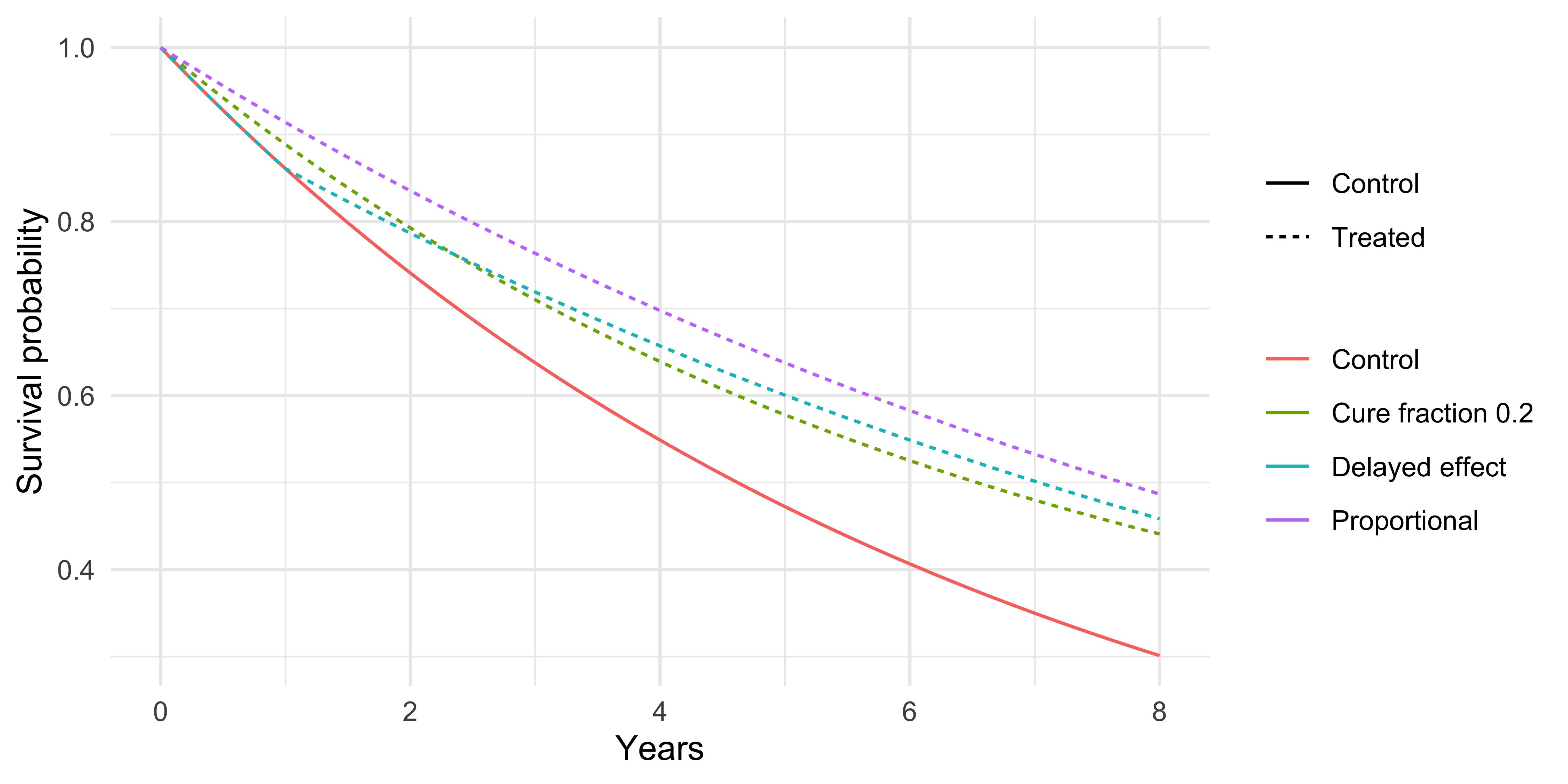
Figure 18.1 shows three scenarios built from the same control arm, a constant hazard of 0.15 per year (median survival 4.6 years). Treatment either cuts the hazard by 40 percent from the start (proportional), cuts it by 40 percent only after a delay of one year, or cures 20 percent of patients and leaves the rest at the control hazard.
Show the R code
tt <-seq(0, 8, by =0.05)S_ctl <-surv_pwexp_S(tt, 0.15)dd <-rbind(data.frame(t = tt, S = S_ctl, arm ="Control", scenario ="Control"),data.frame(t = tt, S =surv_pwexp_S(tt, 0.15*0.6), arm ="Treated", scenario ="Proportional"),data.frame(t = tt, S =surv_pwexp_S(tt, c(0.15, 0.09), c(0, 1)), arm ="Treated", scenario ="Delayed effect"),data.frame(t = tt, S =0.2+0.8* S_ctl, arm ="Treated", scenario ="Cure fraction 0.2"))ggplot(dd, aes(t, S, color = scenario, linetype = arm)) +geom_line() +labs(x ="Years", y ="Survival probability", color =NULL, linetype =NULL) +theme_minimal()
Figure 18.1: Survival curves for a control arm with hazard 0.15 per year and three treatment scenarios: proportional hazards with hazard ratio 0.6, a delay of one year before the same hazard ratio takes effect, and a cure fraction of 0.2.
Three Bayesian responses are in common use.
The first is a piecewise treatment effect, \(\theta_k = -\log\mathrm{HR}_k\) in interval \(k\), with a hierarchical prior that lets the effect change over time but shrinks it toward a common value. It is the piecewise exponential model of Section 18.3 with a treatment effect in each interval, and its posterior answers the clinical question “when does the benefit begin?” directly. The second is a mixture cure model (Boag 1949; Berkson and Gage 1952), in which a fraction \(\pi\) of treated patients are effectively cured and the rest follow the control hazard, \(S_1(t) = \pi + (1-\pi)S_0(t)\) (in the Berkson-Gage model the uncured patients have a survival function of their own, and following the control hazard is a special case; Chen, Ibrahim, and Sinha (1999) give a Bayesian promotion-time (non-mixture) cure model with a surviving fraction). The posterior for \(\pi\) is the quantity a patient cares about, but it is identifiable only if follow-up is long enough for the curve to plateau; with immature data it is dominated by the prior, which has to be stated. The third is to change the estimand to the restricted mean survival time up to a horizon \(\tau\), \[
\mathrm{RMST}(\tau) = \int_0^\tau S(t)\,dt,
\tag{18.3}\] whose posterior is computed from draws of the survival curve. The difference in RMST is the average event-free time gained within \(\tau\), in months or years, which is the unit in which patients and payers think, and it does not require proportional hazards (Royston and Parmar 2011, 2013; Uno et al. 2014). The idea of a restricted mean life is older than these papers (Irwin 1949; Karrison 1987). It does require a horizon, and the choice of \(\tau\) is part of the estimand and must be fixed in the protocol.
Table 18.5: RMST difference over 5 years and cumulative hazard ratio at 5 years for the three scenarios of the figure (control hazard 0.15 per year, hazard ratio 0.6, delay 1 year, cure fraction 0.2). The control arm has RMST 3.52 years.
Scenario
RMST treated
RMST difference
Cumulative HR
proportional
4.03
0.51
0.60
delayed effect
3.82
0.30
0.68
cure model
3.81
0.30
0.73
The scenarios give different RMST gains, 0.51, 0.3 and 0.3 years over five years, and a cumulative hazard ratio at five years of 0.6, 0.68 and 0.73: the hazard ratio is not a constant, which is the point.
Power loss under a delayed effect
How much does the log-rank test lose? The simulation below compares a trial of 300 patients per arm followed for five years, with the control hazard 0.15 per year, under a constant hazard ratio of 0.75 and under a delayed effect with no benefit for two years and a hazard ratio of 0.583 afterward. The two scenarios are matched so that the treated survival at five years is the same, 0.57, so they describe the same final benefit reached by different paths.
Show the R code
set.seed(1507)rpwexp <-function(n, rates, breaks) { # inversion for a piecewise exponential e <-rexp(n); H <-c(0, cumsum(rates[-length(rates)] *diff(breaks))) k <-findInterval(e, H); breaks[k] + (e - H[k]) / rates[k]}sim_power <-function(rates1, breaks1, n =300, tau =5, R =2000) { rej <-numeric(R); ev <-numeric(R)for (r inseq_len(R)) { t0 <-rexp(n, 0.15); t1 <-rpwexp(n, rates1, breaks1) time <-pmin(c(t0, t1), tau); status <-as.integer(c(t0, t1) <= tau) grp <-rep(0:1, each = n) lr <- survival::survdiff(survival::Surv(time, status) ~ grp) z <-sign(lr$obs[1] - lr$exp[1]) *sqrt(lr$chisq) # positive: more events in control rej[r] <- z >qnorm(0.975); ev[r] <-sum(status) }c(power =mean(rej), events =mean(ev))}p_ph <-sim_power(0.15*0.75, 0)p_del <-sim_power(c(0.15, 0.0875), c(0, 2))tab <-data.frame(Scenario =c("Proportional, HR 0.75", "Delayed 2 years, then HR 0.583"),Power =c(p_ph["power"], p_del["power"]), `Mean events`=c(p_ph["events"], p_del["events"]))knitr::kable(tab, digits =c(0, 2, 0))
Table 18.6: Simulated power of the one-sided log-rank test (alpha 0.025), 300 patients per arm, administrative censoring at 5 years, 2,000 replications, with the mean number of events. Treated survival at 5 years is 0.57 in both scenarios.
Scenario
Power
Mean.events
Proportional, HR 0.75
0.68
287
Delayed 2 years, then HR 0.583
0.55
287
The simulated power is 0.68 under the constant hazard ratio and 0.55 under the delayed effect, with a similar number of events, although the five-year survival difference is the same. The Schoenfeld calculation of Table 18.1, which assumes a single hazard ratio, would not have warned about the difference. Two responses are used in practice: a weighted log-rank test (Fleming-Harrington weights (Harrington and Fleming 1982; Fleming and Harrington 1991)) that gives more weight to late events, and a design that states the delayed-effect model, with its simulation, in the protocol. Either choice is made before the trial; choosing the weights after seeing the curves invalidates the type I error. The next subsection shows what the weighted tests recover.
Tests built for a delayed effect
The Fleming-Harrington weighted log-rank test multiplies the contribution of each event time by a weight \(S(t)^\rho\{1 - S(t)\}^\gamma\), where \(S\) is the pooled Kaplan-Meier estimate (Harrington and Fleming 1982; Fleming and Harrington 1991). The choice \(\rho = \gamma = 0\) is the ordinary log-rank test, and \((\rho, \gamma) = (0, 1)\) puts the weight on late events, where a delayed effect shows. A test that is best for one shape of effect can be poor for another, so the combination test takes the largest of several standardized weighted statistics, usually the four with \(\rho, \gamma \in \{0, 1\}\), and refers it to the multivariate normal distribution implied by their correlation (Lee 2007; Lin et al. 2020). This is the MaxCombo test. Table 18.7 repeats the simulation of Table 18.6 with the weighted test and the MaxCombo test, and adds a null scenario to check the level.
Table 18.7: Simulated rejection rate (one-sided 0.025) of the log-rank test, the Fleming-Harrington (0, 1) test and the MaxCombo test of four Fleming-Harrington statistics, 300 patients per arm, administrative censoring at 5 years, 2,000 replications. The first row is the null of identical survival curves.
Scenario
Log-rank
FH(0,1)
MaxCombo
Null, identical curves
0.02
0.02
0.02
Proportional, HR 0.75
0.67
0.55
0.65
Delayed 2 years, then HR 0.583
0.55
0.80
0.74
Under the delayed effect the weighted test has power 0.8 and the MaxCombo test 0.74, against 0.55 for the log-rank test. Under proportional hazards the order reverses (this table is a fresh simulation, so its log-rank figure differs by Monte Carlo error from the 0.68 of Table 18.6): the log-rank test has 0.67, the MaxCombo test gives up a little (0.65) and the late-weighted test gives up more (0.55). That is the trade. A test chosen for one shape wins when the shape is right and loses when it is wrong, and the MaxCombo test pays a smaller premium for not knowing which shape it will meet, although, as the first caution below says, it too can reject when the experimental arm is worse. All three hold the level under the null of identical curves: the rejection rates are 0.024, 0.022 and 0.021 against the nominal 0.025.
Two cautions go with the table. First, these tests are tests of identical survival curves, and the weighted tests can reject when early harm and late benefit cancel in the average, so that a significant result does not by itself mean that patients on average did better; the modestly weighted tests of Magirr and Burman were proposed to control the risk of declaring a uniformly inferior drug superior (Magirr and Burman 2019). Second, the choice among them is a design decision with regulatory weight: the cross-pharma working group’s straw-man guidance (Roychoudhury et al. 2021) treats the choice of test and the plausible non-proportional scenarios as something to settle, with simulation, at the design stage. Restricted mean survival time, the other main alternative, has an empirical record: in 54 oncology trials whose individual patient data were reconstructed from the published curves, the hazard ratio gave on average a larger treatment effect than the ratio of restricted mean survival times (average ratio 1.11, with substantial variation between trials), and the authors recommend that restricted mean survival time be reported routinely (Trinquart et al. 2016). The rule of this chapter is the same for every alternative: the primary test, its weights or horizon, and the simulation under the delayed-effect scenario go in the protocol before the curves are seen.
18.6 Regulation and practice
Four points follow from the guidance landscape.
First, the estimand comes first. Under ICH E9(R1) (International Council for Harmonisation 2019) the hazard ratio, the RMST difference and the survival difference at a landmark time are different estimands, and a Bayesian analysis reports the posterior of the one the protocol names. The five strategies for intercurrent events of Chapter 5 apply: for time to a non-fatal event in the presence of death, the usual choice is a composite (death counts as an event) or a competing-risks treatment, and each leads to a different model.
Second, what exists on non-proportional hazards is thin. We are not aware of an FDA or ICH guidance that sets a required method for non-proportional hazards or for RMST; the closest thing to a consensus document is the straw-man guidance of the cross-pharma working group discussed above (Roychoudhury et al. 2021), which is industry and academic guidance and not regulatory text. The oncology endpoints guidance (U.S. Food and Drug Administration 2018) discusses the endpoints and their biases, and the practice of FDA reviewers, which can be read in public review documents, is to accept pre-specified alternatives to the log-rank test as sensitivity analyses and to scrutinize post hoc ones. The summary of a drug’s effect on the product label is still usually a hazard ratio. This is an area where agreement with the agency at a pre-submission meeting, on the primary analysis and on the sensitivity analyses, matters more than the choice among statistical methods.
Third, the Bayesian elements map onto the existing framework. An informative prior on the log hazard ratio is judged as in Chapter 8 and Chapter 19, and its worth in events is stated as in Section 18.2. The book’s default for a confirmatory adaptive design without borrowing is a Bayesian success criterion calibrated to the type I error by simulation, with the event-time process (accrual, censoring, the NPH model) inside the simulation. The FDA draft Bayesian guidance (U.S. Food and Drug Administration 2026) describes this as one of three routes, the others being direct interpretation of posterior probabilities (for example with borrowing, by agreement with FDA) and decision-theoretic or benefit-risk criteria. The predictive probability of Section 18.4 is a monitoring aid and enters the formal rules only as a pre-specified futility or sample-size criterion.
Fourth, the event count itself is a design element. The final analysis is triggered by the event count, so the data monitoring committee and the sponsor must agree on how events are adjudicated and counted, and the timing rule for an interim analysis must be prespecified, whether by a number of events or by calendar date. If the analysis occurs at an information fraction other than the target, or events overrun the plan, the actual information fraction has to be handled by a prespecified method (for example an alpha-spending function evaluated at the observed fraction).
Key points
The information about a log hazard ratio is one quarter of the number of events, \(\operatorname{Var}(\hat\theta) \approx 4/D\) under 1:1 allocation. Event-driven trials fix \(D\), and the Schoenfeld formula \(D = 4(z_\alpha + z_\beta)^2/(\log\mathrm{HR})^2\) is the sample size formula of Chapter 9 in event units.
A prior with standard deviation \(s_0\) on the log hazard ratio is worth \(4/s_0^2\) events. A prior of standard deviation 0.2 is worth 100 events.
To be 95 percent sure that an observed hazard ratio of 0.8 is below 0.9, a trial needs about 800 events (probability 0.95).
For a constant hazard the posterior is gamma, and posterior summaries of the median survival come from transforming draws. In the worked example the posterior mean median is 4.7 years, not the plug-in 4.62.
Conditional power under the design assumption and under the trend condition on different fixed effects; predictive probability averages over the posterior of the effect: in the worked row with an observed hazard ratio of 0.95 at half the events the three values are 0.35, 0.03 and 0.09.
Under non-proportional hazards a single Cox hazard ratio can depend on censoring and follow-up, so the estimand needs explicit definition. The log-rank test loses power under a delayed effect (simulated 0.55 against 0.68 for a constant hazard ratio), and the RMST difference and the cure fraction are alternatives, each requiring pre-specification.
No FDA or ICH document, to our knowledge, prescribes a method for non-proportional hazards or RMST. ICH E9(R1) requires that whatever summary measure is chosen be defined as an estimand before the trial.
Exercises
Derive Equation 18.1 from the score test for the Cox model with one binary covariate under 1:1 allocation and a hazard ratio near one.
With a \(\mathrm{Gamma}(2, 10)\) prior on the control hazard, recompute the posterior mean and interval for the control arm with 60 events in 400 patient-years. How many events is the prior worth, and how much does it move the median survival?
Reproduce Table 18.4. For the second row, compute the predictive probability if \(D_{\max}\) is increased to 900, and the conditional power under the design assumption.
Under a flat prior, investigate when the predictive probability lies between the two conditional powers. Is it always so when the design hazard ratio is more favorable than the observed one?
Simulate the cure scenario (cure fraction 0.2, control hazard 0.15 per year). Over follow-up of 3, 5 and 8 years, compute the Cox hazard ratio and the RMST difference. Which is more stable as follow-up lengthens?
A protocol specifies a primary analysis by the log-rank test and a “supportive” RMST analysis chosen after the blinded review of the pooled curve. Write the objection a regulator would raise, and the pre-specification that would meet it.
Alexander, Brian M., Jonathan D. Schoenfeld, and Lorenzo Trippa. 2018. “Hazards of Hazard Ratios: Deviations from Model Assumptions in Immunotherapy.”New England Journal of Medicine 378 (12): 1158–59. https://doi.org/10.1056/NEJMc1716612.
Berkson, Joseph, and Robert P. Gage. 1952. “Survival Curve for Cancer Patients Following Treatment.”Journal of the American Statistical Association 47 (259): 501–15. https://doi.org/10.2307/2281318.
Boag, J. W. 1949. “Maximum Likelihood Estimates of the Proportion of Patients Cured by Cancer Therapy.”Journal of the Royal Statistical Society: Series B 11 (1): 15–44. https://doi.org/10.1111/j.2517-6161.1949.tb00020.x.
Breslow, N. 1974. “Covariance Analysis of Censored Survival Data.”Biometrics 30 (1): 89–99. https://doi.org/10.2307/2529620.
Chen, Ming-Hui, Joseph G. Ibrahim, and Debajyoti Sinha. 1999. “A New Bayesian Model for Survival Data with a Surviving Fraction.”Journal of the American Statistical Association 94 (447): 909–19. https://doi.org/10.1080/01621459.1999.10474196.
Fleming, Thomas R., and David P. Harrington. 1991. Counting Processes and Survival Analysis. New York: Wiley.
Freedman, Laurence S. 1982. “Tables of the Number of Patients Required in Clinical Trials Using the Logrank Test.”Statistics in Medicine 1 (2): 121–29. https://doi.org/10.1002/sim.4780010204.
Harrington, David P., and Thomas R. Fleming. 1982. “A Class of Rank Test Procedures for Censored Survival Data.”Biometrika 69 (3): 553–66. https://doi.org/10.1093/biomet/69.3.553.
Holford, Theodore R. 1976. “Life Tables with Concomitant Information.”Biometrics 32 (3): 587–97. https://doi.org/10.2307/2529747.
Ibrahim, Joseph G., Ming-Hui Chen, Yeongjin Gwon, and Fang Chen. 2015. “The Power Prior: Theory and Applications.”Statistics in Medicine 34 (28): 3724–49.
Irwin, J. O. 1949. “The Standard Error of an Estimate of Expectation of Life, with Special Reference to Expectation of Tumourless Life in Experiments with Mice.”Journal of Hygiene 47 (2): 188–89. https://doi.org/10.1017/S0022172400014443.
Kalbfleisch, John D. 1978. “Non-Parametric Bayesian Analysis of Survival Time Data.”Journal of the Royal Statistical Society: Series B 40 (2): 214–21. https://doi.org/10.1111/j.2517-6161.1978.tb01666.x.
Kaplan, E. L., and Paul Meier. 1958. “Nonparametric Estimation from Incomplete Observations.”Journal of the American Statistical Association 53 (282): 457–81. https://doi.org/10.1080/01621459.1958.10501452.
Karrison, Theodore. 1987. “Restricted Mean Life with Adjustment for Covariates.”Journal of the American Statistical Association 82 (400): 1169–76. https://doi.org/10.1080/01621459.1987.10478555.
Lee, Seung-Hwan. 2007. “On the Versatility of the Combination of the Weighted Log-Rank Statistics.”Computational Statistics & Data Analysis 51 (12): 6557–64. https://doi.org/10.1016/j.csda.2007.03.006.
Lin, Ray S., Ji Lin, Satrajit Roychoudhury, Keaven M. Anderson, Tianle Hu, Bo Huang, Larry F. Leon, et al. 2020. “Alternative Analysis Methods for Time to Event Endpoints Under Nonproportional Hazards: A Comparative Analysis.”Statistics in Biopharmaceutical Research 12 (2): 187–98. https://doi.org/10.1080/19466315.2019.1697738.
Magirr, Dominic, and Carl-Fredrik Burman. 2019. “Modestly Weighted Logrank Tests.”Statistics in Medicine 38 (20): 3782–90. https://doi.org/10.1002/sim.8186.
Mantel, Nathan. 1966. “Evaluation of Survival Data and Two New Rank Order Statistics Arising in Its Consideration.”Cancer Chemotherapy Reports 50 (3): 163–70.
Murray, Thomas A., Brian P. Hobbs, Theodore C. Lystig, and Bradley P. Carlin. 2014. “Semiparametric Bayesian Commensurate Survival Model for Post-Market Medical Device Surveillance with Non-Exchangeable Historical Data.”Biometrics 70: 185–91. https://doi.org/10.1111/biom.12115.
Parmar, Mahesh K. B., David J. Spiegelhalter, Laurence S. Freedman, and CHART Steering Committee. 1994. “The CHART Trials: Bayesian Design and Monitoring in Practice.”Statistics in Medicine 13 (13–14): 1297–1312. https://doi.org/10.1002/sim.4780131304.
Peto, Richard, and Julian Peto. 1972. “Asymptotically Efficient Rank Invariant Test Procedures.”Journal of the Royal Statistical Society: Series A 135 (2): 185–207. https://doi.org/10.2307/2344317.
Roychoudhury, Satrajit, Keaven M. Anderson, Jiabu Ye, and Pralay Mukhopadhyay. 2021. “Robust Design and Analysis of Clinical Trials with Nonproportional Hazards: A Straw Man Guidance from a Cross-Pharma Working Group.”Statistics in Biopharmaceutical Research 15 (2): 280–94. https://doi.org/10.1080/19466315.2021.1874507.
Royston, Patrick, and Mahesh K. B. Parmar. 2011. “The Use of Restricted Mean Survival Time to Estimate the Treatment Effect in Randomized Clinical Trials When the Proportional Hazards Assumption Is in Doubt.”Statistics in Medicine 30 (19): 2409–21. https://doi.org/10.1002/sim.4274.
———. 2013. “Restricted Mean Survival Time: An Alternative to the Hazard Ratio for the Design and Analysis of Randomized Trials with a Time-to-Event Outcome.”BMC Medical Research Methodology 13: 152. https://doi.org/10.1186/1471-2288-13-152.
Schoenfeld, David. 1981. “The Asymptotic Properties of Nonparametric Tests for Comparing Survival Distributions.”Biometrika 68 (1): 316–19. https://doi.org/10.1093/biomet/68.1.316.
Schoenfeld, David A. 1983. “Sample-Size Formula for the Proportional-Hazards Regression Model.”Biometrics 39 (2): 499–503. https://doi.org/10.2307/2531021.
Spiegelhalter, David J., Laurence S. Freedman, and Mahesh K. B. Parmar. 1994. “Bayesian Approaches to Randomized Trials.”Journal of the Royal Statistical Society, Series A 157 (3): 357–416. https://doi.org/10.2307/2983527.
Struthers, Cynthia A., and John D. Kalbfleisch. 1986. “Misspecified Proportional Hazard Models.”Biometrika 73 (2): 363–69. https://doi.org/10.1093/biomet/73.2.363.
Trinquart, Ludovic, Justine Jacot, Sarah C. Conner, and Raphaël Porcher. 2016. “Comparison of Treatment Effects Measured by the Hazard Ratio and by the Ratio of Restricted Mean Survival Times in Oncology Randomized Controlled Trials.”Journal of Clinical Oncology 34 (15): 1813–19. https://doi.org/10.1200/JCO.2015.64.2488.
Uno, Hajime, Brian Claggett, Lu Tian, Eisuke Inoue, Paul Gallo, Toshio Miyata, Deborah Schrag, et al. 2014. “Moving Beyond the Hazard Ratio in Quantifying the Between-Group Difference in Survival Analysis.”Journal of Clinical Oncology 32 (22): 2380–85. https://doi.org/10.1200/jco.2014.55.2208.