A trial that asks one question once is rare. Most trials have a primary endpoint and several secondary ones, two or three doses, a handful of prespecified subgroups, and an interim analysis or two. Every additional question is another chance for luck to produce a result that looks like a discovery. A sponsor who reports the best of twenty results as though it were the only one asked has not told the reader how the result was found, and a regulator who approves on it has accepted a risk that nobody measured. Multiplicity is the name for this problem and the family of procedures that controls it is one of the oldest and most settled parts of trial statistics.
This chapter does two things. First, it sets out the traditional apparatus properly, because it is what regulators expect and because it works: familywise error, Bonferroni, Holm, Hochberg, closed testing, fixed-sequence and graphical procedures, and the way guidance asks for the plan to be written. Second, it shows a different way to pay for looking at many things at once. Instead of raising the bar that each result must clear, a hierarchical model lowers the estimate of each result toward what the other results suggest. Both approaches make the sponsor pay for the extra questions. They pay in different currencies, and the difference matters most when the questions are related, which in a clinical program they nearly always are.
The centerpiece is an illustration motivated by a trial that Novick and Grizzle used in 1965 to argue for Bayesian analysis of trial data: four operations for duodenal ulcer. We work through it with the traditional tools and then with a hierarchical model, on the same illustrative recurrence counts (set at the scale of that trial, not transcribed from the 1965 paper).
ImportantRegulatory anchor
ICH E9, Statistical Principles for Clinical Trials (1998) (International Council for Harmonisation 1998), section 5.6 (multiplicity). Multiplicity arises from “multiple primary variables, multiple comparisons of treatments, repeated evaluation over time and/or interim analyses”. When it is present, “the usual frequentist approach to the analysis of clinical trial data may necessitate an adjustment to the type I error”. The guideline asks that the strategy be identified in the protocol and that adjustment always be considered. Section 2.2 asks for the precise definition of the primary variable to be specified in the protocol, to avoid multiplicity concerns from post hoc definitions.
FDA, Multiple Endpoints in Clinical Trials, guidance for industry (final, October 2022) (U.S. Food and Drug Administration 2022). The agency’s working document on endpoints, with the standard procedures (Bonferroni, Holm, Hochberg, fixed-sequence or hierarchical testing, gatekeeping and graphical approaches) and the expectation that the multiplicity strategy is prespecified and that strong control of the familywise error rate is demonstrated for the endpoints that support a claim.
FDA, Master Protocols for Drug and Biological Product Development (revised draft, June 2026), section on type I error. Draft position: FDA “generally does not recommend the use of multiplicity adjustments to strongly control the probability of making at least one type I error across the multiple comparisons of different drugs” in a master protocol, because the expected number of type I errors is the same as in separate trials. The draft’s scope is wider than unrelated drugs: it also generally does not recommend adjustment across comparisons of one drug in different diseases, conditions or disease subtypes when these are distinct clinical objectives (section III.H). Drafts recommend and are not binding.
FDA, Use of Bayesian Methodology in Clinical Trials of Drug and Biological Products (draft, January 2026), and ICH E20 (Step 2 draft, June 2025). Both place the operating characteristics of a Bayesian design, simulated under a prespecified plan, at the center of the submission, which includes the false positive rate of the decision rule over the family of claims the trial can make. Shrinkage across arms or subgroups is a modeling choice that must be justified and examined in sensitivity analyses (see Chapter 3 for the full map and Chapter 14 for how to run the simulations).
10.1 The problem: many chances for luck
Suppose a drug does nothing and we test it on \(k\) independent endpoints, each at one-sided level \(\alpha = 0.025\). The chance that at least one test crosses the bar is one minus the chance that none does:
\[
\Pr(\text{at least one false positive}) = 1 - (1-\alpha)^k .
\tag{10.1}\]
This probability is the familywise error rate (FWER) when all \(k\) null hypotheses are true. For \(k=1\) it is \(0.025\) by design. The next chunk shows how it grows.
Show the R code
k <-c(1, 2, 3, 5, 6, 10, 20, 50)knitr::kable(data.frame(k, 1- (1- alpha)^k, k * alpha), digits =3, col.names =c("Number of tests", "Familywise error", "Bonferroni bound k alpha"), align ="r")
Table 10.1: Probability of at least one false positive among k independent tests of true nulls, each at one-sided 0.025, with the Bonferroni upper bound k alpha.
Number of tests
Familywise error
Bonferroni bound k alpha
1
0.025
0.025
2
0.049
0.050
3
0.073
0.075
5
0.119
0.125
6
0.141
0.150
10
0.224
0.250
20
0.397
0.500
50
0.718
1.250
With twenty independent tests of a useless drug the chance of at least one “significant” result is about \(0.40\). The book’s companion online lab (module 04, https://nytel.ai/testing/04-multiplicity.html) makes the same point with twenty drugs that are exactly as good as placebo. The right-hand column, \(k\alpha\), is the upper bound used by Bonferroni and it is a good approximation while \(k\alpha\) is small.
There are two further points before the procedures. First, independence is neither the best nor the worst case: dependence can make the probability of at least one false positive either larger or smaller than Equation 10.1, depending on its structure. If the tests share a control group or the endpoints are positively correlated, it is typically smaller, but the number of false positives, when there is one, tends to be larger: the errors come in clumps. Second, the formula is about a drug that does nothing. What a regulator wants to prevent is a false claim, and a claim is made on one result or on a combination of results. The family is therefore defined by the claims the sponsor may make, not by the number of tests the statistician happens to run. A statistician who runs forty tests to understand the data but whose protocol says the claim rests on one prespecified comparison has a family of one.
What counts as the family
ICH E9 lists three sources (multiple primary variables, multiple treatment comparisons, repeated evaluation over time and interim analyses) and the practical definition follows from them. The family is the set of hypotheses such that a rejection of any one of them would be presented as evidence of an effect that supports approval or labeling. That makes three things part of the family: alternative primary endpoints (success on any one is enough), the key secondary endpoints for which a labeling claim is sought, and the dose or population comparisons that could each be the basis of approval. Interim looks on the same endpoint are handled by a group sequential boundary, which Chapter 11 covers, and are combined with the cross-endpoint procedures of this chapter as in the protocol paragraph below.
Co-primary endpoints are a different case and need a different explanation. When the claim requires success on all of them, the trial succeeds only if every endpoint is individually significant, and testing each at the full level \(\alpha\) controls the error for that conjunctive claim without any Bonferroni division (an intersection-union test, as in section III.C.1 of the FDA multiple-endpoints guidance). Dividing \(\alpha\) among co-primary endpoints is therefore unnecessary and costs power; the cost of co-primary endpoints lies instead in the power to win on all of them at once, which is lower than the power on any one. Alternative primary endpoints, where success on any one supports the claim, are the case that needs the adjustments of this chapter.
Exploratory endpoints, safety endpoints and descriptive subgroup displays are outside the family because no claim is made on them, and the protocol should say so. Their results can generate hypotheses, and the honest way to report them is with estimates and intervals and no label of significance.
What preserving the option to look costs in patients
The inflation of the bar can be converted into the currency a sponsor understands. Suppose a trial must keep \(K\) analyses open (endpoints, subgroups, per-protocol against intention-to-treat, adjusted against unadjusted) and guarantees at most \(\alpha = 0.025\) for the best of them, whichever one is reported. For independent statistics the exact threshold is the Sidak value \(z_K = \Phi^{-1}((1-\alpha)^{1/K})\) (Bonferroni’s \(\Phi^{-1}(1-\alpha/K)\) is slightly larger). Because the sample size for a given effect and power is proportional to \((z_{\mathrm{crit}} + z_\beta)^2\), the trial must grow by the factor \(n_K/n_1 = ((z_K + z_\beta)/(z_1 + z_\beta))^2\).
Table 10.2: Cost of keeping K analyses open: Sidak threshold at one-sided 0.025, sample size ratio at 80 percent power, and the extra patients required per 1000 enrolled under a single prespecified analysis.
K
z_K
n_K / n_1
Extra per 1000
1
1.96
1.00
0
5
2.57
1.48
485
10
2.80
1.69
693
50
3.29
2.17
1172
100
3.48
2.38
1377
1000
4.05
3.05
2052
Keeping five analyses open costs about 485 extra patients per 1000, and keeping a hundred open costs a trial about 2.4 times the size. With a standardized effect of 0.1 and 80 percent power, a single prespecified analysis needs about 1570 patients per arm, so the same effect with \(K = 100\) needs roughly 3,730. For Gaussian statistics with nonnegative correlations the Sidak threshold is conservative, so correlated analyses have an effective \(K\) below the nominal count and the table is an upper bound; under negative correlations the Sidak error can exceed its nominal level, and Bonferroni, which needs no dependence assumption, is the safe choice. The table is the argument for prespecifying few analyses, and it is also the reason to price the many analyses that cannot be avoided by modeling (Section 10.4).
10.2 The traditional toolbox
Bonferroni
The simplest procedure: with \(k\) hypotheses and a familywise level \(\alpha\), test each at \(\alpha/k\) (the inequality is Bonferroni’s, Dunn (Dunn 1961) made it a multiple-comparison method, and Dunnett (Dunnett 1955) gave an exact procedure based on the multivariate \(t\) distribution for several treatments against one control, the multi-arm trial case, which is less conservative than Bonferroni because it uses the correlation induced by the shared control). Equivalently, multiply each \(p\)-value by \(k\) and compare to \(\alpha\). The union bound guarantees that the probability of any false rejection is at most \(\alpha\), whatever the dependence between the tests. That guarantee is the reason Bonferroni is in every guidance and every statistical analysis plan: it needs no assumption and its logic can be explained to a clinician in one sentence.
Its cost is power. For \(k=6\) the per-test level is \(0.025/6 = 0.00417\), and the critical value moves from \(z=1.96\) to \(z=2.64\). A trial sized for 90% power at the unadjusted level has noticeably less than that after adjustment, and the lost power is the price of protecting against the case where all six nulls are true. When one or two of the hypotheses are in fact true effects, Bonferroni is paying to guard against errors that cannot occur.
Holm
Holm (1979) is a uniform improvement. Order the \(p\)-values \(p_{(1)}\le\dots\le p_{(k)}\). Compare \(p_{(1)}\) to \(\alpha/k\); if it is rejected, compare \(p_{(2)}\) to \(\alpha/(k-1)\); continue until a \(p\)-value fails, and then stop and retain that hypothesis and all remaining ones. Holm controls the familywise error rate in the strong sense, with no assumption on dependence, and it rejects everything Bonferroni rejects and sometimes more. There is no good reason to use plain Bonferroni when Holm is available, other than that Bonferroni’s simplicity helps in a protocol that must be read by many people.
Hochberg
Hochberg (1988) runs the order in the other direction: start from the largest \(p\)-value and compare it with \(\alpha\), the next largest with \(\alpha/2\), and so on; at the first \(p_{(j)} \le \alpha/(k-j+1)\) reject that hypothesis and all with smaller \(p\)-values. It is a step-up version of Holm’s step-down test and rejects at least as many hypotheses. The price is an assumption: the guarantee holds when the test statistics are independent or positively dependent in a specific sense (positive dependence such as nonnegative correlation among one-sided normal test statistics, which covers comparisons with a shared control). Its step-up logic rests on the Simes inequality (Simes 1986), and Hommel (Hommel 1988) gave a more powerful procedure under the same conditions. FDA’s guidance on multiple endpoints states these conditions and does not treat Hochberg as assumption-free.
Here are the three procedures on one set of \(p\)-values, with the package functions mult_bonferroni(), mult_holm() and mult_hochberg().
Table 10.3: Hypotheses rejected at one-sided 0.025 by the unadjusted, Bonferroni, Holm and Hochberg procedures for six p-values.
Hypothesis
p-value
Unadjusted
Bonferroni
Holm
Hochberg
E1
E1
0.004
reject
reject
reject
reject
E2
E2
0.011
reject
E3
E3
0.019
reject
E4
E4
0.022
reject
E5
E5
0.041
E6
E6
0.300
At the unadjusted level four of the six pass. All three adjusted procedures reject only E1, whose \(p\)-value \(0.004\) is just under \(0.025/6 = 0.0042\); after that Holm’s next threshold is \(0.025/5 = 0.005\), which \(0.011\) misses, so it stops. The three procedures give the same answer here and separate when several \(p\)-values are small, for example \(0.004, 0.005, 0.006\) and the rest large.
Closed testing
The procedures above are special cases of one principle due to Marcus, Peritz and Gabriel (1976). A closed test starts from the family of hypotheses \(H_1,\dots,H_k\) and forms all intersection hypotheses (for example, “\(H_1\) and \(H_3\) are both true”). Each intersection is tested with any valid level-\(\alpha\) test. An individual hypothesis \(H_i\) is rejected if every intersection that contains \(H_i\) is rejected at level \(\alpha\). This controls the familywise error rate strongly, because a true intersection of nulls is only wrongly rejected with probability at most \(\alpha\), and any false rejection of an individual hypothesis requires rejecting the intersection of all true nulls. Holm’s procedure is the closed test that uses Bonferroni for each intersection. Choosing a more powerful intersection test, such as one that uses the correlation between endpoints, gives a more powerful closed procedure, and that is where the modern literature on multiplicity lives (Dmitrienko and D’Agostino 2013 gives a full survey).
For a clinician the lesson is that “the multiplicity adjustment” is not a single formula. It is a rule for how a result about one hypothesis is allowed to depend on results about the others, and it is chosen at the protocol stage. The same logic yields the gatekeeping and fixed-sequence procedures that dominate practice.
Fixed-sequence (hierarchical) testing
Order the hypotheses in advance by clinical importance: \(H_1, H_2, \dots, H_k\). Test \(H_1\) at the full \(\alpha\). If it is rejected, test \(H_2\) at the full \(\alpha\), and so on. Stop at the first failure and do not test the rest. The familywise error rate is controlled at \(\alpha\) without any division of the level, because at most one hypothesis can be the first true null, and it is tested at \(\alpha\).
This is the most common strategy for a primary endpoint followed by key secondaries, and it is what “primary/secondary hierarchy” means in a protocol. The price is that the order is final. A secondary endpoint late in the sequence can be tested at full level only if everything before it succeeded, so a failure on the primary, or on an early secondary, makes all later results exploratory regardless of how impressive they look. This is the right behavior for a regulator and it often surprises a clinical team, which has seen a large effect on endpoint 4 and expects to say something about it.
Two consequences follow for how the hierarchy is written. First, the sponsor should put first the endpoint on which it is most confident of success and which carries the claim that matters most, since a failure ends the chain. Second, the sequence can be a tree and not a line: “if the primary succeeds, test secondary A and secondary B each at \(\alpha/2\), and if A succeeds, test A’s follow-up at \(\alpha/2\) plus whatever passes from B.” That is a graphical procedure.
Graphical procedures
Bretz, Maurer, Brannath and Posch (2009) gave a framework that unifies Bonferroni, Holm, fixed sequence, fallback and gatekeeping procedures in one picture. Each hypothesis is a node with a weight \(w_i\) (its share of \(\alpha\), with \(\sum w_i \le 1\)). Directed edges carry weights \(g_{ij}\) giving the fraction of \(H_i\)’s level that passes to \(H_j\) if \(H_i\) is rejected. The algorithm is: reject any \(H_i\) with \(p_i \le w_i\alpha\); remove it, pass its weight along the edges, update the edge weights, and repeat. The result controls the familywise error rate strongly, because each step is a closed-test shortcut. Burman, Sonesson and Guilbaud (Burman, Sonesson, and Guilbaud 2009) developed a parallel recycling framework, Bretz and colleagues (Bretz et al. 2011) extended graphs to Simes and parametric tests, and Maurer and Bretz (Maurer and Bretz 2013) showed how to combine a graph with group sequential looks, which is where this chapter meets Chapter 11.
The method is popular because the graph is the protocol: a statistician can draw it for the clinical team, the team can see which results unlock which, and the same picture goes into the statistical analysis plan. Here is a small example with two primary endpoints and two secondaries. Each primary gets half the level; if a primary is rejected, its level passes to the secondary that clinically follows it; once a secondary is rejected, its level passes to the other primary.
Table 10.4: Hypotheses rejected by the graphical procedure in three scenarios of p-values for two primary and two secondary endpoints.
Scenario
Rejected
P1 strong, P2 weak, S1 moderate
P1, P2, S1
P1 weak, others strong
P1, P2, S1, S2
all marginal
In the first scenario \(P1\) is rejected at \(0.0125\), which passes its weight to \(S1\); \(S1\) (\(p=0.010\)) is rejected at \(0.0125\) and passes its weight to \(P2\), which now has the full level and rejects at \(p=0.020\). \(S2\) (\(p=0.30\)) stays. In the second, \(P1\) at \(0.020\) fails alone, but \(P2\) is rejected and passes to \(S2\), which is rejected and returns its level to \(P1\), which then clears \(0.025\), and \(S1\) follows. The third is the reminder that a single common marginal \(p\)-value of \(0.015\) is not enough when each primary has only half of the level, \(0.0125\), and nothing unlocks. The operating characteristics of the whole graph can be simulated as in Chapter 14.
Gatekeeping procedures, in which a family of primary hypotheses must be passed before a secondary family is tested (Dmitrienko, Offen and Westfall (Dmitrienko, Offen, and Westfall 2003) is the standard reference for the case where not every primary effect must be significant), are special cases of such graphs. The harder practical question is how a graph meets the interim analyses of Chapter 11, since an outcomes trial has both a key secondary hierarchy and a group sequential design. Take a trial with H1 (the primary composite) and H2 (all-cause death, tested only after H1). At the start the whole level 0.025 sits on H1 and H2 has weight zero. If H1 is rejected at an interim look, at the level its spending function allows there, its weight moves to H2, which is then tested from that look onward, with its own spending function applied to the information H2 has accumulated and not to the information H1 had at the time of the transfer. This is the setting of Maurer and Bretz (Maurer and Bretz 2013), who showed how to combine a graph with group sequential looks, and of the recycling framework of Burman, Sonesson and Guilbaud (Burman, Sonesson, and Guilbaud 2009); the details of the spending rule are theirs to fix and the protocol has to state the version chosen. For the protocol this means three statements that the graphical description above must be supplemented by: the spending function for each hypothesis, the rule that a transferred weight is spent from the look at which the transfer happens, and the graph with its weights printed. A design that says only “alpha is spent by O’Brien-Fleming” has left the key secondary undefined.
What the guidance asks for
The EMA’s guidance is older and shorter. The Points to Consider on multiplicity issues (CPMP/EWP/908/99) was adopted in 2002 and took legal effect on 1 April 2003 (European Medicines Agency, Committee for Proprietary Medicinal Products 2002). A draft replacement guideline (EMA/CHMP/44762/2017) went to public consultation in 2017 and, as far as the EMA’s page shows, remains a draft (European Medicines Agency, Committee for Medicinal Products for Human Use 2017); its summary says it adds or updates the treatment of multiplicity in safety, drug-response studies, secondary endpoints, subgroup analysis and estimation. A draft recommends and does not bind, so a European submission is still read against the 2002 document and ICH E9. ICH E9 section 5.6 is short and gives the principle: identify multiplicity in the protocol and consider adjustment. It also asks that the key primary variable and critical treatment contrast be identified in advance, which is a form of multiplicity control without any adjustment at all: a family of one. The FDA guidance on multiple endpoints (final, October 2022) is the detailed companion. It describes the situations (multiple primary endpoints and the claims that follow from them, co-primary endpoints that must all succeed (each tested at the full level), primary and secondary endpoints, composite endpoints with components) and the procedures above, and it expects strong control of the familywise error rate for the endpoints that will support a claim.
TipIn the protocol: the multiplicity paragraph
State, before unblinding: (1) the family of hypotheses, by name, with the claim each supports; (2) the testing procedure (fixed sequence, Holm, a graph; include the graph); (3) the familywise level, usually one-sided \(0.025\); (4) how interim analyses on each endpoint consume that level (reference the alpha-spending function from Chapter 11); (5) which endpoints are exploratory and will be reported without significance claims; (6) the rule for what happens to later hypotheses when an earlier one fails; (7) if subgroups are prespecified for claims, where they sit in the graph. Strong control of the familywise error rate needs a proof for an analytically controlled procedure, or calibration by simulation over the relevant mixed null configurations (some hypotheses true, others false), effect magnitudes and nuisance parameters, with a stated justification for the least favorable scenarios; the global null alone is not enough. That simulation, and the power for each hypothesis under the planned scenarios, belong in the SAP appendix.
10.3 Subgroups and the forking paths
Of all the sources of multiplicity, the subgroup analysis is the one that most often misleads. A trial that fails overall will be examined by age, sex, region, baseline severity, biomarker status and prior therapy. With twelve ways to slice the data, luck has twelve chances. The classic warning is the ISIS-2 trial (ISIS-2 (Second International Study of Infarct Survival) Collaborative Group 1988), which enrolled 17,187 patients with suspected myocardial infarction. To illustrate the problem, its authors showed that when patients were split by astrological birth sign, aspirin appeared to have no benefit for patients born under Gemini or Libra, although in the trial as a whole aspirin reduced vascular mortality very strongly. The point is not that Gemini is special. It is that twelve signs gave twelve chances and two came up as an apparent exception. Module 04 of the companion lab repeats the exercise with a made-up useless drug split twelve ways.
A subgroup finding has a structure that makes it worse than a simple count suggests. The analyst who sees a promising subgroup usually chose how to cut: age above or below 65, or 60, or 70; ejection fraction by tertiles or by a threshold; region by country or by continent. Gelman and Loken (2014) called this the garden of forking paths: even if the analyst ran only one test, the choice of which test depended on the data, and the effective number of comparisons is the number of tests that would have been run had the data looked different. The multiplicity is hidden in decisions, not in the number of \(p\)-values. This is the practical reason ICH E9 insists on defining the primary variable and analysis in the protocol, and why post hoc subgroup claims are treated as hypothesis-generating.
A reader who needs a standard for reporting subgroup analyses in a trial paper will find one in Wang and colleagues (2007): say how many subgroup analyses were done, state which were prespecified, and test for interaction between the subgroup variable and treatment rather than comparing \(p\)-values inside subgroups (a significant effect in one subgroup and a non-significant effect in another is not evidence that the effects differ). The interaction test has little power at the usual sample size, so the honest result of most subgroup analyses is “consistent with a common effect”.
The traditional remedies are to prespecify a small number of subgroups with a rationale, to include the subgroup variable in the multiplicity graph when a claim is intended, to test interaction first, and to treat everything else as exploratory. Those remedies work and should be used. They have a limitation that the Bayesian alternative addresses: they are all-or-nothing. A subgroup is either in the family or out of it, and the estimate in a subgroup that is outside the family is reported at face value, with all the noise that implies.
Why a Bayesian must also ask how the result was chosen
A Bayesian analysis conditions on the data it is shown, and that is where the forking paths matter. The regulator does not see the sponsor’s data \(X\). It sees a message \(M = \varsigma(X)\), where the reporting rule \(\varsigma\) (which subgroup, which endpoint, which analysis) is chosen by the sponsor.
NoteProposition (selected likelihood)
Let \(X\) have density \(p(x \mid \theta)\) and let the sponsor report \(M = \varsigma(X)\), with \(\varsigma\) possibly randomized. The regulator’s posterior is \(p(\theta \mid M = m) \propto p(\theta)\, \mathcal{L}_\varsigma(\theta; m)\), where \(\mathcal{L}_\varsigma(\theta; m)\) is the density at \(m\) of the distribution of \(\varsigma(X)\) under \(\theta\) (the pushforward of \(p(x \mid \theta)\) through \(\varsigma\), with respect to a dominating measure for the reports, and averaging over any randomization), so it depends on \(\varsigma\). If \(\varsigma\) reports the largest of \(K\) independent components \(X_1, \dots, X_K\), the likelihood of the reported value \(m\) is \[
\mathcal{L}_\varsigma(\theta; m) = \sum_{k=1}^{K} p(m \mid \theta_k) \prod_{j \ne k} F(m \mid \theta_j),
\tag{10.2}\] with \(F\) the distribution function of a component. In the upper tail \(F(m \mid \theta_j) \to 1\), so for exchangeable components the ratio of \(\mathcal{L}_\varsigma\) to the naive likelihood \(p(m \mid \theta_k)\) approaches \(K\).
The proof is the density of a maximum of independent variables. The consequence is that the naive likelihood \(p(m \mid \theta_k)\) is the wrong likelihood for the reported value. A factor that does not depend on \(\theta\) cancels from posterior odds, so the ratio approaching \(K\) is not itself a \(K\)-fold distortion of the evidence. The distortion is in how \(\mathcal{L}_\varsigma\) depends on \(\theta\). Take the simplest case, a common effect \(\theta \sim N(0, 1)\) and \(K\) independent \(N(\theta, 1)\) components, of which only the maximum \(m\) is reported. The correct likelihood is \(K\phi(m - \theta)\Phi(m - \theta)^{K-1}\) and the naive one is \(\phi(m - \theta)\), so the correct one carries the extra factor \(\Phi(m - \theta)^{K-1}\), which falls as \(\theta\) rises and pulls the posterior down. For \(m = 2\) and \(K = 5\) the posterior mean of \(\theta\) is 1 under the naive likelihood and 0.59 under the correct one, and the posterior probability that \(\theta > 0\) falls from 0.92 to 0.85. The regulator cannot compute the correct posterior without knowing \(\varsigma\). This, and not any claim that posteriors depend on intentions, is the Bayesian reason for a protocol: the protocol is the specification of \(\varsigma\).
It also shows what is right and what is beside the point in the familiar Bayesian retort that optional stopping does not affect the posterior (see Chapter 12 for the calibration side of that argument). The retort is correct when the full sample path is reported, because then \(M = X\) and \(\varsigma\) is the identity. It is beside the point when the report is a summary chosen after the fact, because then \(\varsigma\) is not the identity and the sponsor knows something the regulator does not. Shrinkage, below, is the Bayesian way to put the selection into the model by giving the whole family of subgroups one prior, instead of reporting the winner alone.
10.4 The Bayesian alternative: shrinkage instead of threshold inflation
The idea
A Bonferroni correction makes the evidence required for each result higher, and it does so independently of what the other results say. That is a strange property when the results are related. If six subgroup effects look similar, that is information that each of them is probably close to their average. If one is large and five are near zero, that is information that the large one is probably a mix of effect and luck. A hierarchical (multilevel) model uses this information. It treats the effects \(\theta_1,\dots,\theta_k\) of the \(k\) arms, doses or subgroups as draws from a common distribution,
where \(\hat\theta_j\) is the observed effect (for example a log odds ratio), \(s_j\) its standard error, \(\mu\) the common mean and \(\tau_g\) the between-group standard deviation. For fixed \(\mu\) and \(\tau_g\), the posterior mean for each group is a weighted average of its own estimate and the common mean,
This is partial pooling. A group with a small standard error (much information) stays near its own estimate. A group with a large standard error (little information) is pulled toward the mean. When \(\tau_g\) is large, the groups are nearly unrelated and little pooling occurs; when \(\tau_g\) is small, the groups behave as one, and the model reproduces the pooled analysis. The data inform \(\tau_g\), but the amount of pooling also depends on the exchangeability assumption, the distributional form of the group effects and, in a full Bayesian analysis, the hyperprior; it is not free of assumptions. In a full Bayesian analysis the posterior mean integrates over the posterior of \(\mu\) and \(\tau_g\), so Equation 10.4 is its conditional form. (In a full Bayesian analysis, \(\mu\) and \(\tau_g\) have priors. With few groups, the prior for \(\tau_g\) should be weakly informative and examined in sensitivity analysis. Chapter 8 discusses how. Chapter 19 returns to the same hierarchical structure for borrowing across trials and baskets.)
The consequence for multiplicity is that the correction for looking at many things is built into the estimate. The largest of \(k\) observed effects is on average too large, because it was selected as the largest, and the hierarchical estimate pulls it back toward the mean by about the right amount. A posterior statement about the selected group is then made with honest uncertainty, without any change to the threshold. Gelman, Hill and Yajima (2012; see also Gelman and Tuerlinckx 2000 for the Type S error analysis that preceded it) make this argument in the language of applied statistics: when estimates are partially pooled, multiple comparisons stop being a problem that needs a separate fix, because the problem was that unpooled estimates are noisier than they should be. Berry and Berry (2004) applied the same idea to adverse events in a drug safety trial, where hundreds of event types are examined and the hierarchical model borrows strength across them.
Stein, Efron and Morris, and the batting averages
There is a classical theorem behind shrinkage, and its scope should be stated exactly. Stein (1956) showed that for three or more means in a multivariate normal model with known variances, the usual estimate, each group’s own average, is inadmissible under total squared-error loss: there is an estimator that has smaller total squared error whatever the true means are, and James and Stein (James and Stein 1961) gave one explicitly. The theorem concerns that model and that loss. It does not establish that the empirical-Bayes fit used for the ulcer analysis below improves every arm, the selected contrast, posterior coverage or a clinical decision; that analysis is a separate model-based procedure whose performance has to be assessed, as the simulation below does for one case. Efron and Morris (1975, 1977) made this concrete with a data set of baseball players’ early-season batting averages, where the estimates shrunk toward the league mean predicted the rest of the season better than the raw averages did for most players, and the improvement came largely from the extreme players. The same logic applies to the player who hits 1 for 19 against one pitcher: against a bar of “a probability of one in a hundred if his true average is \(0.300\)”, it looks like evidence he cannot hit that pitcher, but there are many pitchers, and a hierarchical analysis of the player’s record across all of them gives an estimate for that pitcher that is lower than average but much nearer to it than \(1/19\). The batting average problem is a multiplicity problem in a form everyone has intuition for: look at enough batter and pitcher pairs and some pair will look like a curse.
A numerical illustration: the winner’s curse
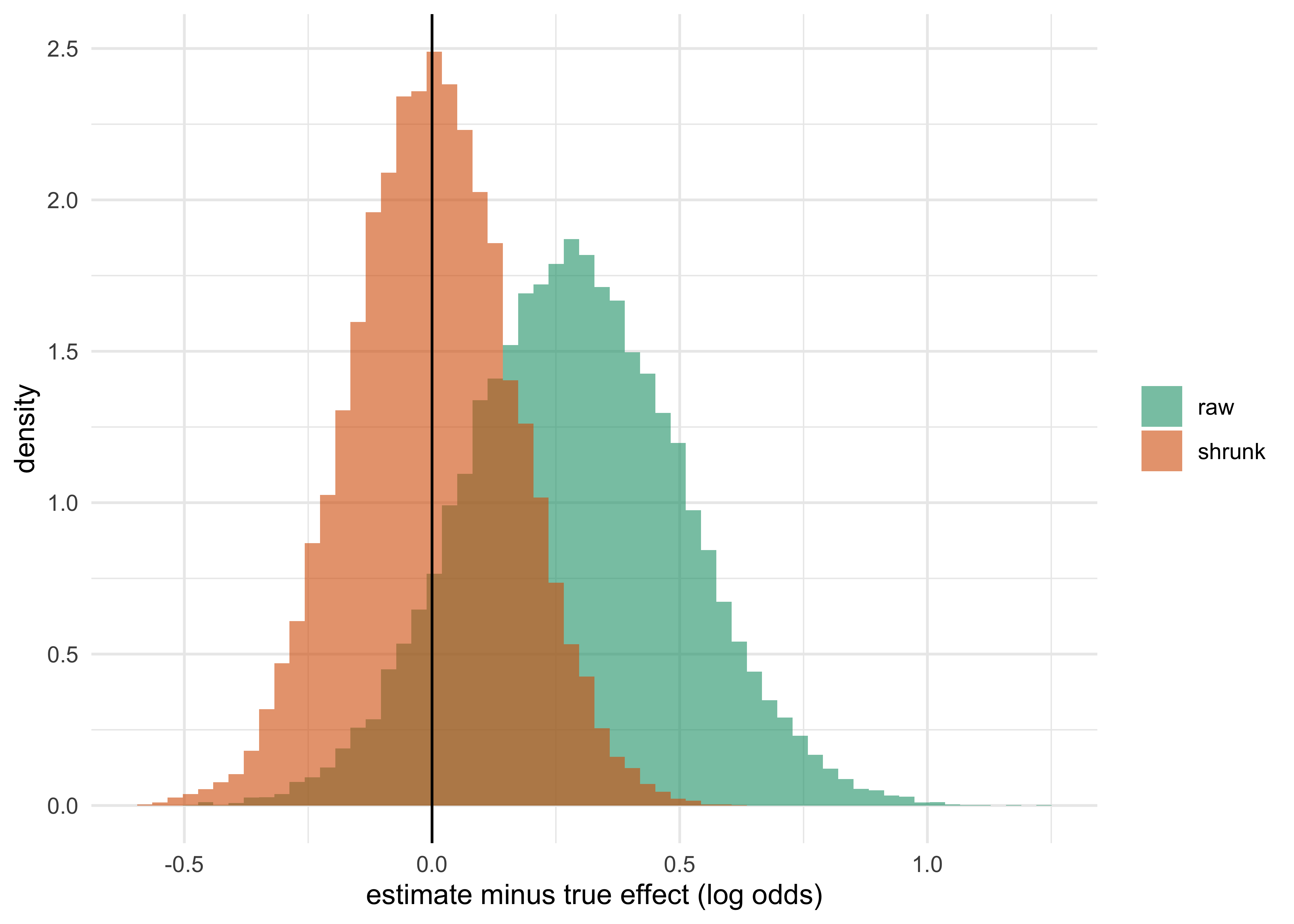
The reason shrinkage answers selection bias can be seen in a short simulation. Six arms have true effects drawn from \(N(0, 0.2^2)\) on the log odds scale, each estimated with standard error \(0.28\) (about what the ulcer trial’s arms give, below). The trial reports the arm with the largest observed effect. How wrong is that arm’s raw estimate, and how wrong is the shrunken one?
Show the R code
set.seed(3); k <-6; reps <-20000; tau <-0.2; se <-0.28th <-matrix(rnorm(reps * k, 0, tau), reps); y <- th +matrix(rnorm(reps * k, 0, se), reps)i <-cbind(1:reps, max.col(y)); B <- se^2/ (tau^2+ se^2) # shrinkage factor, mu = 0 knownerr <-data.frame(raw = y[i] - th[i], shrunk = (1- B) * y[i] - th[i])wc <-sapply(err, function(e) c(mean_error =mean(e), rmse =sqrt(mean(e^2))))ggplot(stack(err), aes(values, fill = ind)) +geom_histogram(aes(y =after_stat(density)), bins =60, alpha =0.6, position ="identity") +geom_vline(xintercept =0) +scale_fill_brewer(palette ="Dark2", name =NULL) +labs(x ="estimate minus true effect (log odds)", y ="density") +theme_minimal()
Figure 10.1: Error of the estimate for the apparently best of six arms. The raw estimate is biased upward because the arm was selected for looking best. The shrunken estimate is centered on the truth with a much smaller spread.
The raw estimate of the selected arm is too high by about 0.29 on the log odds scale on average and its root mean squared error is about 0.36. The shrunken estimate has no average bias and a root mean squared error of about 0.16. Here the true between-arm spread \(\tau_g\) was known; in a real trial it is estimated, which adds uncertainty, and the fitted model is only as good as the exchangeability assumption behind it. The qualitative point stands. The correction for selection is an estimate that is smaller and more honest, and not a harder test applied to an estimate that is still biased.
What shrinkage does not do
It does not control the familywise error rate, and a regulator who requires strong control of that rate for a claim will not be satisfied by a posterior probability alone. Chapter 14 shows how to calibrate the Bayesian decision rule, with its shrinkage in place, so that the familywise error rate over the family of claims is controlled at the required level, and reports the result as simulated operating characteristics. When this is done, the hierarchical rule usually has more power than Bonferroni at the same simulated familywise error rate if the effects are related, because the threshold does not have to be raised by the full factor of \(k\). When the effects are unrelated (a single true effect among many nulls), shrinkage toward the common mean works against the one real effect, and a good hierarchical design uses a heavier-tailed or mixture distribution for the group effects so that one large outlier is not pulled all the way in. That robustness is also a choice to be justified in the protocol and tested by simulation. Two platform trials that handle multiplicity by modeling and not by adjustment, I-SPY 2 and REMAP-CAP, are described in the “In practice” section below.
The comparison, then, is not “Bayes avoids multiplicity” but a different division of labor. The traditional procedure sets a threshold that guarantees the error rate, whatever the effects are, and pays in power. The Bayesian procedure uses the structure of the effects to estimate more accurately, and then, if the regulator requires it, is calibrated to the same error rate by simulation, with the power gain realized to the extent that the structure is real.
Where familywise control is not the target: false discovery rate and prior probabilities
The two halves of this chapter, thresholds and shrinkage, meet when the aim is a screen and not a claim. For hundreds of biomarkers, signatures or adverse event terms the aim is to find most of the real signals and to tolerate a known share of false leads. Benjamini and Hochberg (Benjamini and Hochberg 1995) defined the false discovery rate, the expected proportion of false rejections among the rejections, and gave a step-up procedure: order the \(p\)-values, find the largest \(j\) with \(p_{(j)} \le jq/m\), and reject the hypotheses with the \(j\) smallest \(p\)-values. It controls the rate at \(q\) for independent \(p\)-values and under positive dependence of the kind that supports Hochberg’s procedure (Benjamini and Yekutieli 2001). Table 10.5 applies the procedures of this chapter and the Benjamini-Hochberg procedure to simulated screens of 1000 hypotheses, 100 of them with a true effect (a \(z\) statistic centered at 3), all at the level 0.025, averaged over 1000 replications.
Table 10.5: Average results over 1000 simulated screens of 1000 hypotheses, 100 with a true effect (z statistic centered at 3), at the level 0.025 for each procedure. Rejected, False and True are the mean numbers of hypotheses rejected, of rejections that are true nulls, and of real effects found. Realized FDR is the mean over screens of the proportion of false rejections among the rejections (zero when nothing is rejected).
Rejected
False
True
Realized FDR
Unadjusted
107.6
22.7
85.0
0.209
Bonferroni
14.3
0.0
14.3
0.002
Holm
14.4
0.0
14.4
0.002
Benjamini-Hochberg
50.1
1.2
48.9
0.022
On average Bonferroni and Holm reject 14.3 and 14.4 hypotheses with 0.02 and 0.02 false rejections, Benjamini-Hochberg rejects 50.1 with 1.2 false, a realized false discovery rate of 0.022 against the nominal 0.025, and the unadjusted test rejects 107.6 with 22.7 false, a realized rate of 0.21.
The Bayesian reading of the same screen is Efron’s two-groups model (Efron 2008): each statistic comes from the null with probability \(\pi_0\) and from an alternative otherwise, and the local false discovery rate is the posterior probability of the null given the statistic. The Benjamini-Hochberg procedure thresholds an estimate of the tail-area false discovery rate, with the null proportion set to one. Berry and Hochberg (D. A. Berry and Hochberg 1999) set out the Bayesian view of multiple comparisons, in which a hierarchical prior supplies the correction without a change of threshold. Scott and Berger (Scott and Berger 2006, 2010) show where the correction comes from: if the prior probability that a hypothesis is a true effect is itself unknown and is learned from all the hypotheses, the posterior imposes a penalty that grows with the number of hypotheses when few signals are present among many hypotheses, and the penalty relaxes as more signals appear.
In practice false discovery rate control is used for screening, exploratory endpoints and signal detection, where no confirmatory claim is made, for example the double false discovery rate flagging of adverse events of Mehrotra and Adewale (Mehrotra and Adewale 2012), and it is not used for a confirmatory claim, which stays under familywise control as in the guidance above.
A large trial with many subgroups: RECOVERY
The same machinery applies when the groups are prespecified subgroups of one large trial. Chapter 22 reanalyzes the RECOVERY dexamethasone result with a hierarchical model across its prespecified subgroups, with the prior on the between-subgroup standard deviation \(\tau_g\) stated explicitly, the posterior median of \(\tau_g\) reported (the posterior of \(\tau_g\) depends on its prior), and age-adjusted rate ratios. The subgroup estimates move toward the overall effect in proportion to how little information each carries, which is the winner’s-curse correction of the previous section applied to a trial that actually did report subgroups. The reader should take from it the sensitivity of the shrinkage to the prior on \(\tau_g\) as much as the shrunken estimates themselves.
10.5 An illustration motivated by the four-operation ulcer trial
The original
Novick and Grizzle (1965) made one of the first cases for Bayesian analysis of clinical trial data using an experiment then in progress that compared four operative treatments for duodenal ulcer. The structure is the one on which the traditional apparatus does worst: four arms, hence six pairwise contrasts; a trial in progress, so repeated analysis; and a modest effect on a binary endpoint. They argued that a Bayesian analysis conditions on the data in hand and therefore needs neither a multiplicity correction nor a spending schedule, and that prior information about operative outcomes can be stated rather than suppressed. The feature of the trial we use is structural: the four operations differ in how much stomach is removed, so they are ordered.
The counts below are illustrative, set at the scale of that trial and not transcribed from the 1965 paper, with recurrence decreasing in the extent of resection. They are the counts used in Polson and Sokolov’s working paper (Polson and Sokolov 2026) and ship with the package as the dataset ulcer.
Show the R code
l <-shrink_logodds(ulcer); y <- l$y; v <- l$vknitr::kable(transform(ulcer, rate =round(100* recurrences / n, 1), log_odds =round(y, 3), se =round(sqrt(v), 3)), col.names =c("Operation", "Patients", "Recurrences", "Recurrence rate (%)", "Log odds", "Standard error"), align ="r")
Table 10.6: Illustrative duodenal ulcer data: recurrences by operation, with the recurrence rate, log odds and its standard error.
Operation
Patients
Recurrences
Recurrence rate (%)
Log odds
Standard error
Drainage and vagotomy
96
20
20.8
-1.335
0.251
25 per cent resection and vagotomy
104
16
15.4
-1.705
0.272
50 per cent resection and vagotomy
110
12
10.9
-2.100
0.306
75 per cent resection
107
9
8.4
-2.388
0.348
NoteA note on the companion lab
Module 05 of the companion lab uses a different table for the same trial: four treatments (named A to D) with 100 patients each and a three-level outcome (excellent, fair, death), described there as “the 1965 data as used in Polson and Sokolov (2026)”. The working paper itself says its counts are illustrative and recurrence-based, so the companion lab’s table and this chapter’s table are not the same data. Both illustrate the same lesson, and the numbers in this chapter come from the code shown.
What the traditional reading does with it
Show the R code
d <- y[1] - y[4]; se <-sqrt(v[1] + v[4]); z <- d / se; p2 <-2* (1-pnorm(z))ulcer_std <-c(log_OR = d, se = se, Z = z, p_two_sided = p2, bonferroni_6 =min(1, 6* p2), bar_z =qnorm(1-0.025/6))
The best against worst contrast, drainage and vagotomy against 75 percent resection, is a difference of \(12.4\) percentage points in the recurrence rate, a log odds ratio of 1.053 with standard error 0.43. The test statistic is \(Z = 2.45\) and the unadjusted two-sided \(p\)-value is 0.0142. That is the answer if this single contrast was the only one asked. It was not: with four arms there are six pairwise contrasts, and the best against worst is the one that was chosen because it is the largest.
The Bonferroni-adjusted \(p\)-value is 0.0855, and the finding is not reportable. A group sequential design with four interim analyses at the corrected level would put the first boundary at \(5.34\) (an O’Brien-Fleming boundary at the Bonferroni level, from Polson and Sokolov’s script), which \(Z=2.45\) does not approach. An e-value procedure at the same corrected level, with a normal-mixture alternative of prior scale 0.5 on the log odds ratio, would need \(Z\ge 4.53\) (the construction is in Chapter 12). Every one of these procedures returns nothing from a twelve point difference in recurrence. It is worth being fair to the traditional tools here: they are doing what they promise. If the question really were “does any of these six contrasts show a difference, with a guarantee that I will make a false claim at most one time in forty”, the answer from this trial is “not established”. The difficulty is that this is the wrong question for the clinicians who ran the trial, and the correction is not informative about the question they care about.
Holm does not rescue it. With six contrasts and the best one’s \(p\)-value adjusted by \(6\), Holm and Bonferroni agree on the smallest \(p\)-value; Holm’s gain would come from the other contrasts, none of which is stronger. The pairwise Bonferroni and Holm procedures do not use the ordering visible in the table (the recurrence rate falls steadily as more stomach is removed); a prespecified trend test does.
What the hierarchical reading does with it
Show the R code
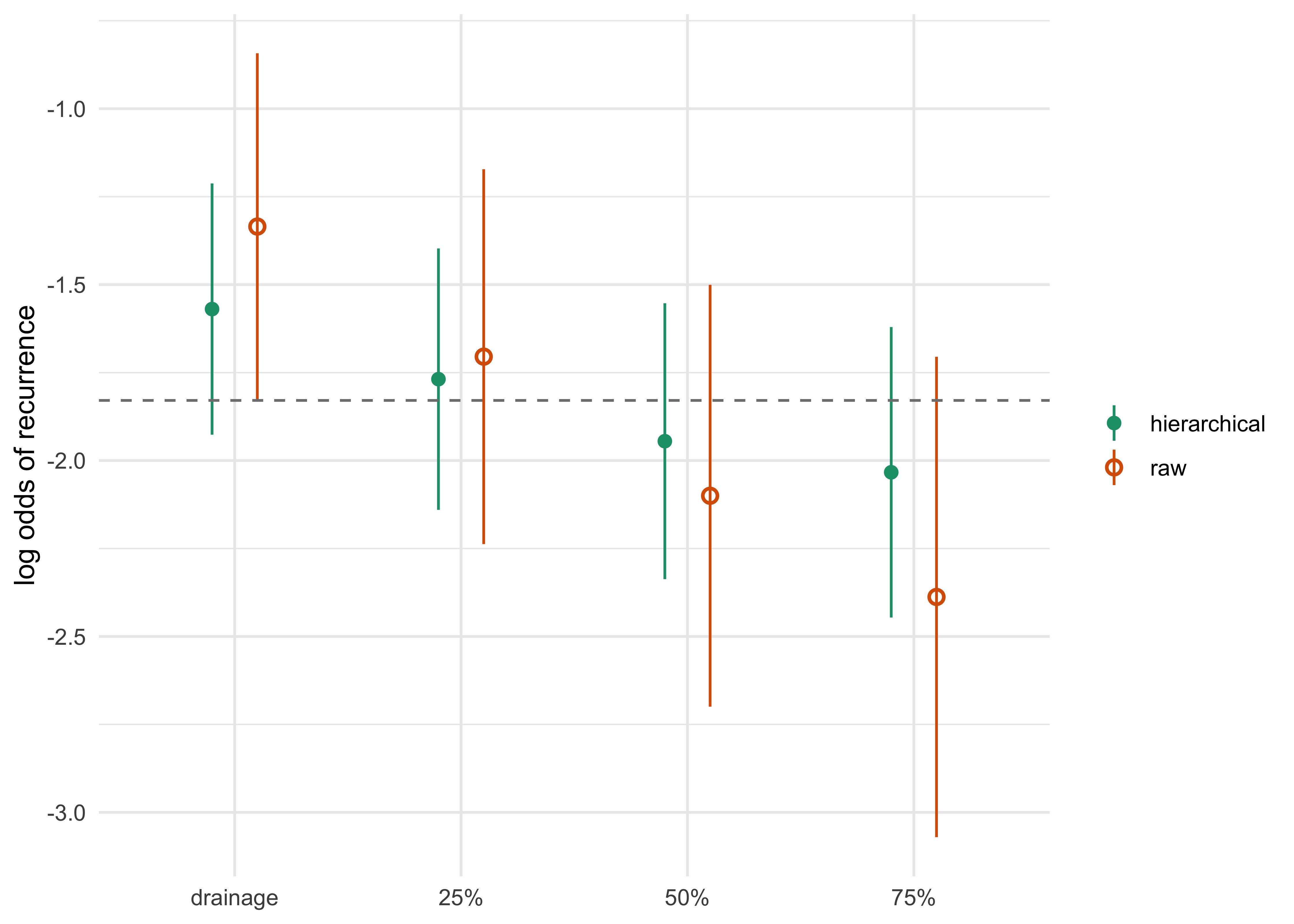
f <-shrink_eb_fit(y, v); ds <- f$shrunk[1] - f$shrunk[4]; ss <-sqrt(f$sd[1]^2+ f$sd[4]^2)ulcer_hier <-c(mu = f$mu, tau = f$tau, shrunk_contrast = ds, sd = ss, pr_drainage_worse =pnorm(ds / ss))op <-c("drainage", "25%", "50%", "75%")df <-data.frame(op =factor(rep(op, 2), op), kind =rep(c("raw", "hierarchical"), each =4),est =c(y, f$shrunk), half =1.96*c(sqrt(v), f$sd))ggplot(df, aes(op, est, colour = kind, shape = kind)) +geom_pointrange(aes(ymin = est - half, ymax = est + half), position =position_dodge(0.4)) +geom_hline(yintercept = f$mu, linetype =2, colour ="grey50") +scale_shape_manual(values =c(16, 1), name =NULL) +scale_colour_brewer(palette ="Dark2", name =NULL) +labs(x =NULL, y ="log odds of recurrence") +theme_minimal()
Figure 10.2: Four operations for ulcer: raw log odds of recurrence (open circles) and hierarchical posterior means (filled), with 95% intervals. The arms with the least information are pulled toward the common mean.
The Bayesian analysis also pays for having four arms, but it pays in the estimate and not in the threshold. A hierarchical model across the four operations, as in Equation 10.3, with \(\tau_g\) estimated by marginal likelihood, gives a between-arm standard deviation of 0.264 on the log odds scale, which shrinks each arm roughly half way to the common mean. The fit is shrink_eb_fit() in the package.
The best against worst contrast falls from 1.053 to 0.464 with posterior standard deviation 0.278, and the posterior probability that drainage and vagotomy is worse than 75 percent resection is 0.952. This is the number a clinician can use: the chance that the less extensive operation really has the higher recurrence rate. It was computed from the same data as the Bonferroni-adjusted \(p\)-value of \(0.0855\) and on a scale where it can be compared with the success criterion \(\Pr(\delta > a \mid \text{data}) > c\) of the FDA Bayesian draft (Chapter 7).
Notice that the Bayesian answer is not permissive. The Bayesian point estimate of the difference is less than half the raw one. What differs is that the analysis reports where the evidence stands instead of discarding it, and that it reports the quantity a decision maker needs. A posterior probability of \(0.952\) is not a claim of statistical significance under strong familywise error control, and it should not be presented as one. Whether it would meet a prespecified threshold \(c\) is a question for the design, answered by simulation (Chapter 14).
The estimate of \(\tau_g\) here rests on four arms, which is thin, and it is the sensitive part of the analysis. With four groups the data say little about \(\tau_g\) and a plug-in estimate treats it as known. A fully Bayesian analysis would integrate uncertainty in the hierarchy’s parameters; its interval and its sensitivity to the prior scale should be reported, and the sensitivity of the 0.952 to the prior on \(\tau_g\) is the first thing a reviewer will ask about. This is part of the cost of the approach and is itemized in the side-by-side table below.
Structure that the correction cannot see
The four operations are ordered by extent of resection, so the scientific question is a monotone trend. A single prespecified contrast carrying a linear trend carries no multiplicity burden at all.
Show the R code
w <-c(-1.5, -0.5, 0.5, 1.5) # equally spaced scores for extent of resectiontr <-sum(w * y); se_tr <-sqrt(sum(w^2* v)); z_tr <- tr / se_trpp <-shrink_post_prob(-tr, se_tr, 0.5)$prob # prior sd 0.5 on the trendlbf <--0.5*log(1+0.5^2/ se_tr^2) +0.5* (tr / se_tr^2)^2/ (1/ se_tr^2+1/0.5^2)ulcer_trend <-c(trend = tr, se = se_tr, Z = z_tr, p_one_sided =pnorm(z_tr), post_prob = pp, log_BF = lbf)
The linear trend is -1.777 with standard error 0.676, so \(Z=-2.63\) and the one-sided \(p\)-value is 0.0043. It is immune to the Bonferroni argument, since it is a single comparison chosen from the design and not from the data. Under a prior of scale \(0.5\) on the weighted sum (a prior standard deviation of 0.1 per step, which is a skeptical choice) the posterior probability that the prespecified linear trend contrast is negative is 0.941, with \(\log \mathrm{BF} = 1\). This is a statement about one weighted sum of log odds. It can hold even when adjacent recurrence rates reverse direction, so it is not the posterior probability that recurrence is monotone in extent of resection; that would need a joint model and the joint ordering event.
This result is available to a traditional analysis too, and it is the point of the section: a single prespecified trend test (or any contrast that encodes the ordering, such as the Williams or Bartholomew procedures used for ordered dose-response) is a traditional remedy and a good one. What the Bayesian framework adds is that the same structure can be built into the model, with a monotone dose-response or an ordered hierarchical prior on the arm effects, so that the final analysis uses the ordering and still reports the pairwise comparisons that a clinician wants. Dose finding (Chapter 17) takes this idea much further.
The two ways to pay for looking
Both paradigms must pay for examining four arms, and for examining them repeatedly. The standard design pays by raising the bar. Bonferroni divides the level, spending functions raise the early boundaries, and the normal-mixture e-value construction adds an approximately constant surcharge. The Bayesian design pays by moving the estimate: hierarchical shrinkage pulls each arm toward the common mean in proportion to how little information it carries. Multiplicity adjustment limits confirmatory claims; the estimates and intervals remain available. Shrinking the estimate uses the information in the comparison, and uses the other arms as well.
Traditional (Holm, graph, fixed sequence)
Hierarchical Bayesian
What the protocol fixes
The family, the procedure and graph, the level \(\alpha\)
The model, the prior on \(\tau_g\), the decision rule on a posterior probability
How looking at many things is paid for
A raised bar (smaller per-test level) or an ordered gate
A shrunken estimate, in proportion to the evidence in each arm
Error guarantee
Strong control of FWER by construction
By simulation under the prespecified design (Chapter 14)
Uses the relatedness of arms
Only through the correlation in some closed tests
Directly, through \(\tau_g\)
Uses ordering of doses
Trend test or a gate; or not at all
Monotone or ordered prior
Main risk
Low power when many hypotheses are tested and effects are related
Over-shrinkage when one arm is truly different; sensitivity to the prior on \(\tau_g\)
What the regulator asks
Is the graph prespecified and is the FWER controlled?
Is the exchangeability assumption plausible, what is the simulated FWER and power, how sensitive are results to \(\tau_g\)?
Where they agree
With a flat prior, a normal likelihood and one comparison, the posterior probability of benefit is one minus the one-sided \(p\)-value, so the thresholds agree
Where the traditional design is the better choice: a confirmatory trial with two or three prespecified endpoints and a sponsor who needs a clean familywise error statement for each claim. A fixed-sequence or graphical procedure delivers exactly that, is understood by every review division, and needs no modeling decision that the agency can dispute. The Bayesian hierarchical approach earns its place when there are many related groups (doses, subgroups, baskets, arms of a platform), when an estimate for each group is wanted and not only a decision on a family, and when borrowing across groups is in the sponsor’s interest and the exchangeability assumption can be defended.
10.6 Across arms and across drugs: platforms
Multiple arms in one trial raise a question that a single-drug trial does not: what is the family? FDA’s June 2026 revised draft guidance on master protocols takes a position that surprises people who learned multiplicity from the textbook. For comparisons of different drugs against a common control, the agency “generally does not recommend the use of multiplicity adjustments to strongly control the probability of making at least one type I error across the multiple comparisons of different drugs”. The reason given is that the expected number of type I errors is the same whether those comparisons are made in independent trials or in one master protocol. A hypothetical sponsor of two unrelated drugs that run two separate trials does not adjust either one for the other, so there is no reason to adjust when they happen to share a protocol. The argument has a long history outside master protocols. Rothman (Rothman 1990) argued that no adjustments are needed for multiple comparisons at all, and Proschan and Waclawiw (Proschan and Waclawiw 2000) gave practical guidelines for when adjustment is warranted. The book’s rule, here and in the rest of the chapter, is that the claim defines the family: adjust when one claim rests on the best of several comparisons. The different-drug comparisons described here can constitute separate families. Distinct endpoint claims for one drug do not, by themselves, justify dispensing with multiplicity control. The position is for unrelated drugs, often from different sponsors, and, in the draft’s wording, generally also for comparisons of one drug in different diseases, conditions or disease subtypes when these represent distinct clinical objectives, as in separate basket substudies. It is not for multiple doses or regimens of one drug, which are alternative ways to support one claim and sit within the usual family, and it is not a licence to select subgroups or baskets and then combine them to support a single claim, which returns to the usual family. It is a draft. Chapter 20 develops the shared control, the non-concurrent control question and the way hierarchical models are used across arms and across subgroups in platform trials.
The consequences are two. First, in a platform with several drugs the multiplicity question becomes a question about which comparisons form a family, and that is decided by claims, as in the rest of this chapter. Second, shrinkage across drugs, where the model treats different drugs as exchangeable draws, is a different question from multiplicity adjustment, and it needs its own justification: unrelated drugs are not exchangeable in any scientific sense, and shrinking one drug’s effect toward the average of others borrows from the wrong place. Hierarchical modeling is natural for doses of the same drug, for subgroups of the same population, and for baskets of tumor types with a common mechanism. It is not natural for a list of unrelated products. The hierarchical designs actually used for subgroups and baskets, the Thall and colleagues model for diseases with several subtypes, the Berry and colleagues subpopulation models and the exchangeability-nonexchangeability model, are described with their priors on the between-group variance and their simulated error rates in Section 19.13.
10.7 Seeing it in the lab
TipTry it in the lab: module 04, many tests, false alarms
Go to https://nytel.ai/testing/04-multiplicity.html. Before you press anything, predict how many false alarms you will see in 1,000 trials of a useless drug with 5 tests at the unadjusted cutoff, then run it. Repeat with Bonferroni and with the fixed order, and compare the climb curve with Table 10.1. The package function mult_simulate() runs the same experiment in R.
TipTry it in the lab: module 05, the ulcer trial
Go to https://nytel.ai/testing/05-ulcer-trial.html. Pick the best and worst treatments in the table, predict whether the chi-square test and the pairwise comparison agree, and then check. Note that the lab uses its own three-outcome table for the trial, so the numbers differ from Table 10.6; the lesson, that picking the extreme pair after the fact fools you far more often than the nominal level suggests, is the same.
10.8 In practice: multiplicity handled by modeling
Large platform trials ask many questions at once, and the two examples below are among the best documented cases in which the multiplicity is addressed in the statistical model and a high decision threshold, and not by a familywise adjustment. Neither claims strong familywise control, and neither should be read as showing that the Bayesian machinery of this chapter is a regulatory substitute for it.
I-SPY 2: ten signatures per drug
I-SPY 2, a neoadjuvant breast cancer platform, evaluates each experimental drug in ten prospectively defined biomarker signatures (all patients, HR+, HR-, HER2+, HER2-, MammaPrint high-2, and the four HER2 by HR combinations). A drug is therefore tested in ten overlapping subgroups, which is exactly the subgroup problem of Section 10.3. The design does not adjust the threshold ten ways. Estimates come from a covariate-adjusted logistic model for pathologic complete response (covariates HER2, HR and MammaPrint), and a drug graduates in a signature when its Bayesian predictive probability of success in a hypothetical 300-patient equally randomized phase 3 trial reaches 85% (Park et al. 2016). The threshold is set high on purpose, and the authors state that a drop between the interim and final predictive probability “was anticipated in the I-SPY 2 design and led to our setting a high threshold of 85%”. A drug is dropped for futility only if its predictive probability is below 10% in all ten signatures.
Neratinib shows what this looks like. With 115 neratinib patients and 78 concurrent controls it graduated in one signature only, HER2+/HR-: estimated pCR 56% (95% probability interval 37 to 73%) against 33% (11 to 54%) for the trastuzumab control, probability of superiority 95%, final predictive probability of phase 3 success 79%. It did not graduate in HER2+/HR+ (30% against 17%, predictive probability 65%) or in all HER2+ patients (39% against 23%, predictive probability 73%). The lesson for this chapter: the answer a clinician needs, in which of the ten signatures does the drug work, is reported as an estimate with an interval for each, and the selection of the best signature is guarded by a demanding decision rule and the shared model, with the operating characteristics established by simulation before the trial (Chapter 14). The graduation is a screening decision that routes a drug to a confirmatory trial, and not a claim of efficacy for labeling. The exact graduation rule is revisited in Chapter 20.
REMAP-CAP: hierarchical modeling across domains and arms
REMAP-CAP, the adaptive platform for severe pneumonia, evaluates interventions in several domains at once with a single Bayesian cumulative logistic model for organ support-free days. In its interleukin-6 receptor antagonist comparison, the model adjusts for site, age, sex and time epoch, uses neutral priors on the treatment effects, and nests tocilizumab and sarilumab under a shared hierarchical prior on an overall IL-6 antagonist effect, so each drug borrows from the other in proportion to how alike their data are (REMAP-CAP Investigators et al. 2021). The decision triggers are posterior probabilities: efficacy if the probability that the odds ratio exceeds 1.0 against control is above 99%, futility if the probability that it exceeds 1.2 is below 5%. The chronology and the effect estimates are in Chapter 20.
The two-drug hierarchy is the shrinkage of Section 10.4 in a small case: sarilumab, with few patients, is held nearer the common IL-6 effect than its own data would put it, and the 99% efficacy bar is the high threshold that stands in for a per-comparison adjustment. The lesson is the one in Section 10.6: the two drugs share a mechanism, so borrowing between them is defensible, whereas the domains evaluating unrelated treatments are not pooled in the same way. FDA’s draft master protocol guidance does not generally recommend adjusting across different drugs, so the justification for the shrinkage must come from the science of the shared mechanism.
The FDA master protocol position
As set out in Section 10.6, the June 2026 revised draft on master protocols does not recommend strong familywise control across comparisons of different drugs. It does not remove the need to define the family for doses, regimens and subgroups that support a single claim (separate basket substudies with distinct objectives are different from selecting subgroups to support one claim), and it does not make a posterior probability a substitute for a calibrated error rate. I-SPY 2 and REMAP-CAP both fit within that position because their per-drug decisions are not claims of a familywise kind, but any labeling claim based on a signature or a pooled effect would return to the questions of the family and of simulated operating characteristics raised earlier in this chapter.
10.9 Reporting and review: what to expect
A reviewer who sees a multiplicity section will ask a short list of questions, and the answers should be written into the protocol and SAP before unblinding.
What is the family, and what claim does each hypothesis support? Is the testing procedure prespecified in enough detail that two statisticians would reach the same set of rejections from the same \(p\)-values? If a graph is used, does the SAP show the initial weights and transition weights, and has the graph been simulated for the planned scenarios? How do interim analyses for each endpoint consume the level? What is the status of the secondary endpoints if the primary fails? Which subgroups are prespecified, and is there an interaction test?
For a design that uses hierarchical shrinkage, add: what is the exchangeability assumption and why is it plausible; what prior is used for the between-group standard deviation \(\tau_g\) and what happens to the decisions if that prior is changed; what is the simulated probability of a false claim over the family, across the relevant mixed null configurations (some groups null, others active), effect magnitudes and nuisance parameters, with a stated justification for the least favorable scenarios (hierarchical borrowing can make a mixed configuration worse than the global null); and what is the power for each group when effects are related and when only one group is active. These are the simulated operating characteristics that the FDA Bayesian draft and ICH E20 ask for, and they are the currency in which the saving from shrinkage is demonstrated. A hierarchical design that has not been calibrated in this way is an analysis plan for a regulator to doubt, however sensible the model.
Estimates matter as much as tests. A forest plot of subgroup results should show the shrunken estimates next to the raw ones when a hierarchical model is used, and should show intervals, not asterisks. The extreme subgroups are the ones that move most, and a reader can see at once which findings survive the correction for looking.
Key points
The chance of at least one false positive among \(k\) independent tests at level \(\alpha\) is \(1-(1-\alpha)^k\); for \(k=20\) at \(0.025\) it is about \(0.40\). The family is defined by the claims the trial may make, not by the number of tests run.
Holm uniformly beats Bonferroni with the same dependence-free guarantee. Hochberg is more powerful but needs positive dependence. Closed testing is the principle behind both, and fixed-sequence and graphical procedures are closed tests with a clinically ordered structure that the protocol can draw.
ICH E9 section 5.6 and the FDA multiple endpoints guidance (final, October 2022) ask for the strategy to be prespecified, for one key primary variable where possible, and for strong control of the familywise error rate on the claims. Hypotheses outside the family are exploratory.
Subgroups and the forking paths hide multiplicity in analyst choices. Prespecify few, test for interaction, report intervals, and treat the rest as hypothesis generating.
Hierarchical shrinkage pays for looking at many groups in the estimate, using the other groups as information; Bonferroni pays in the threshold and ignores them. Stein’s result says the raw estimates are inadmissible under total squared-error loss for three or more normal means, which is a statement about that model and loss, not a guarantee for any fitted procedure.
In the four-operation ulcer example the Bonferroni-adjusted \(p\)-value for best against worst is \(0.0855\), while the hierarchical posterior probability that drainage is worse than 75 percent resection is \(0.952\) on a contrast shrunk from \(1.053\) to \(0.464\); a prespecified monotone trend has \(p=0.0043\) and needs no correction.
Shrinkage does not give a familywise error guarantee. When a regulator requires one, calibrate the Bayesian rule by simulation and report the operating characteristics (Chapter 14).
FDA’s master protocols draft generally does not recommend multiplicity adjustment across different drugs in a platform, or across one drug’s distinct clinical objectives; shrinkage across unrelated drugs is not justified by that position and is a separate modeling choice (Chapter 20).
Prefer a single prespecified contrast that encodes the structure (ordered doses, a monotone trend) to a bag of pairwise tests.
I-SPY 2 (ten signatures per drug, 85% predictive-probability graduation, neratinib graduating only in HER2+/HR-) and REMAP-CAP (hierarchical IL-6 antagonist effect, 99% efficacy trigger) handle multiplicity by modeling and a demanding threshold, not a familywise adjustment.
NoteDiscussion questions
A trial has a primary endpoint and four key secondary endpoints. The team proposes testing the four secondaries at \(\alpha/4\) each, regardless of the primary. Why might a fixed-sequence or graphical procedure be better for the claims the sponsor cares about, and what would the team lose by moving to it?
In the ulcer example the Bonferroni-adjusted \(p\)-value is \(0.0855\) and the hierarchical posterior probability is \(0.952\). A regulator asks which number the sponsor would put in the label. What would you say, and what additional work would you do to make the Bayesian number acceptable?
A subgroup analysis shows a large benefit in patients under 65 and none above. List the questions you would ask before believing the interaction, including the ones about how the cut point was chosen.
When is the exchangeability assumption behind partial pooling plausible across doses, subgroups, baskets and drugs, and what would you examine to check it? What happens to the shrunken estimate of the one truly active group when the others are inert?
FDA’s master protocols draft does not generally recommend adjustment across different drugs on a platform. Why does that argument not extend to several doses of one drug tested against the same control, if the sponsor wants to claim any of them?
Benjamini, Yoav, and Yosef Hochberg. 1995. “Controlling the False Discovery Rate: A Practical and Powerful Approach to Multiple Testing.”Journal of the Royal Statistical Society: Series B (Methodological) 57 (1): 289–300.
Benjamini, Yoav, and Daniel Yekutieli. 2001. “The Control of the False Discovery Rate in Multiple Testing Under Dependency.”The Annals of Statistics 29 (4): 1165–88. https://doi.org/10.1214/aos/1013699998.
Berry, Donald A., and Yosef Hochberg. 1999. “Bayesian Perspectives on Multiple Comparisons.”Journal of Statistical Planning and Inference 82 (1–2): 215–27. https://doi.org/10.1016/s0378-3758(99)00044-0.
Berry, Scott M., and Donald A. Berry. 2004. “Accounting for Multiplicities in Assessing Drug Safety: A Three-Level Hierarchical Mixture Model.”Biometrics 60 (2): 418–26. https://doi.org/10.1111/j.0006-341X.2004.00186.x.
Bretz, Frank, Willi Maurer, Werner Brannath, and Martin Posch. 2009. “A Graphical Approach to Sequentially Rejective Multiple Test Procedures.”Statistics in Medicine 28 (4): 586–604. https://doi.org/10.1002/sim.3495.
Bretz, Frank, Martin Posch, Ekkehard Glimm, Florian Klinglmueller, Willi Maurer, and Kornelius Rohmeyer. 2011. “Graphical Approaches for Multiple Comparison Procedures Using Weighted Bonferroni, Simes, or Parametric Tests.”Biometrical Journal 53 (6): 894–913. https://doi.org/10.1002/bimj.201000239.
Burman, Carl-Fredrik, Christian Sonesson, and Olivier Guilbaud. 2009. “A Recycling Framework for the Construction of Bonferroni-Based Multiple Tests.”Statistics in Medicine 28 (5): 739–61. https://doi.org/10.1002/sim.3513.
Dmitrienko, Alex, and Ralph B. D’Agostino. 2013. “Traditional Multiplicity Adjustment Methods in Clinical Trials.”Statistics in Medicine 32 (29): 5172–5218. https://doi.org/10.1002/sim.5990.
Dmitrienko, Alex, Walter W. Offen, and Peter H. Westfall. 2003. “Gatekeeping Strategies for Clinical Trials That Do Not Require All Primary Effects to Be Significant.”Statistics in Medicine 22 (15): 2387–2400. https://doi.org/10.1002/sim.1526.
Dunnett, Charles W. 1955. “A Multiple Comparison Procedure for Comparing Several Treatments with a Control.”Journal of the American Statistical Association 50 (272): 1096–1121. https://doi.org/10.1080/01621459.1955.10501294.
Efron, Bradley. 2008. “Microarrays, Empirical Bayes and the Two-Groups Model.”Statistical Science 23 (1): 1–22. https://doi.org/10.1214/07-sts236.
Efron, Bradley, and Carl Morris. 1975. “Data Analysis Using Stein’s Estimator and Its Generalizations.”Journal of the American Statistical Association 70 (350): 311–19.
———. 1977. “Stein’s Paradox in Statistics.”Scientific American 236 (5): 119–27.
Gelman, Andrew, Jennifer Hill, and Masanao Yajima. 2012. “Why We (Usually) Don’t Have to Worry about Multiple Comparisons.”Journal of Research on Educational Effectiveness 5 (2): 189–211. https://doi.org/10.1080/19345747.2011.618213.
Gelman, Andrew, and Eric Loken. 2014. “The Statistical Crisis in Science.”American Scientist 102 (6): 460. https://doi.org/10.1511/2014.111.460.
Gelman, Andrew, and Francis Tuerlinckx. 2000. “Type S Error Rates for Classical and Bayesian Single and Multiple Comparison Procedures.”Computational Statistics 15 (3): 373–90. https://doi.org/10.1007/s001800000040.
Hochberg, Yosef. 1988. “A Sharper Bonferroni Procedure for Multiple Tests of Significance.”Biometrika 75 (4): 800–802. https://doi.org/10.1093/biomet/75.4.800.
Holm, Sture. 1979. “A Simple Sequentially Rejective Multiple Test Procedure.”Scandinavian Journal of Statistics 6 (2): 65–70. https://www.jstor.org/stable/4615733.
Hommel, G. 1988. “A Stagewise Rejective Multiple Test Procedure Based on a Modified Bonferroni Test.”Biometrika 75 (2): 383–86. https://doi.org/10.1093/biomet/75.2.383.
ISIS-2 (Second International Study of Infarct Survival) Collaborative Group. 1988. “Randomised Trial of Intravenous Streptokinase, Oral Aspirin, Both, or Neither Among 17,187 Cases of Suspected Acute Myocardial Infarction: ISIS-2.”The Lancet 332 (8607): 349–60. https://doi.org/10.1016/S0140-6736(88)92833-4.
James, W., and Charles Stein. 1961. “Estimation with Quadratic Loss.” In Proceedings of the Fourth Berkeley Symposium on Mathematical Statistics and Probability, Volume 1: Contributions to the Theory of Statistics, 361–79. Berkeley, Calif.: University of California Press.
Marcus, Ruth, Eric Peritz, and K. Ruben Gabriel. 1976. “On Closed Testing Procedures with Special Reference to Ordered Analysis of Variance.”Biometrika 63 (3): 655–60. https://doi.org/10.1093/biomet/63.3.655.
Maurer, Willi, and Frank Bretz. 2013. “Multiple Testing in Group Sequential Trials Using Graphical Approaches.”Statistics in Biopharmaceutical Research 5 (4): 311–20. https://doi.org/10.1080/19466315.2013.807748.
Mehrotra, Devan V., and Adeniyi J. Adewale. 2012. “Flagging Clinical Adverse Experiences: Reducing False Discoveries Without Materially Compromising Power for Detecting True Signals.”Statistics in Medicine 31 (18): 1918–30. https://doi.org/10.1002/sim.5310.
Novick, Melvin R., and James E. Grizzle. 1965. “A Bayesian Approach to the Analysis of Data from Clinical Trials.”Journal of the American Statistical Association 60 (309): 81–96.
Park, John W., Minetta C. Liu, Douglas Yee, Christina Yau, Laura J. van ’t Veer, W. Fraser Symmans, Melissa Paoloni, et al. 2016. “Adaptive Randomization of Neratinib in Early Breast Cancer.”New England Journal of Medicine 375 (1): 11–22. https://doi.org/10.1056/NEJMoa1513750.
Polson, Nicholas G., and Vadim Sokolov. 2026. “Bayesian Versus Standard Clinical Trial Design: Theory, Evidence, and Protocol.”
Proschan, Michael A., and Myron A. Waclawiw. 2000. “Practical Guidelines for Multiplicity Adjustment in Clinical Trials.”Controlled Clinical Trials 21 (6): 527–39. https://doi.org/10.1016/s0197-2456(00)00106-9.
REMAP-CAP Investigators, Anthony C. Gordon, Paul R. Mouncey, Farah Al-Beidh, Kathryn M. Rowan, Alistair D. Nichol, et al. 2021. “Interleukin-6 Receptor Antagonists in Critically Ill Patients with Covid-19.”New England Journal of Medicine 384 (16): 1491–1502. https://doi.org/10.1056/NEJMoa2100433.
Scott, James G., and James O. Berger. 2006. “An Exploration of Aspects of Bayesian Multiple Testing.”Journal of Statistical Planning and Inference 136 (7): 2144–62. https://doi.org/10.1016/j.jspi.2005.08.031.
———. 2010. “Bayes and Empirical-Bayes Multiplicity Adjustment in the Variable-Selection Problem.”The Annals of Statistics 38 (5): 2587–2619. https://doi.org/10.1214/10-aos792.
Simes, R. J. 1986. “An Improved Bonferroni Procedure for Multiple Tests of Significance.”Biometrika 73 (3): 751–54. https://doi.org/10.1093/biomet/73.3.751.
Stein, Charles. 1956. “Inadmissibility of the Usual Estimator for the Mean of a Multivariate Normal Distribution.” In Proceedings of the Third Berkeley Symposium on Mathematical Statistics and Probability, 1:197–206. https://www.degruyter.com/document/doi/10.1525/9780520313880-018/html.
Wang, Rui, Stephen W. Lagakos, James H. Ware, David J. Hunter, and Jeffrey M. Drazen. 2007. “Statistics in Medicine: Reporting of Subgroup Analyses in Clinical Trials.”New England Journal of Medicine 357 (21): 2189–94. https://doi.org/10.1056/NEJMsr077003.