Every statistical analysis of a trial rests on assumptions that are not in the data, and the Bayesian analysis is distinguished mainly by the fact that it writes one of them down. That is also the objection to it. A sponsor who proposes a prior is proposing a number that a reviewer can attack, and a reviewer who has never been asked to attack the implicit assumptions of a power calculation may find the explicit ones easier to see. This chapter is about making the prior something a sponsor can state, justify, quantify and defend, in the form a regulator will ask for it.
We begin with the traditional design, which has a prior of its own that rarely gets that name. We then ask where a prior comes from in a sponsor’s program, and why the apparently safe choice of a flat prior is often the least defensible one. We describe the three classical reference priors (skeptical, enthusiastic and noninformative), the conditional means prior that lets a clinician specify a prior on the scale she can think on, and the effective sample size that says in patients how much a prior weighs. We close with prior-data conflict, sensitivity analysis and the tipping-point prior, and with what the FDA’s January 2026 draft says about all of it. Chapter 6 supplied the machinery (prior, likelihood, posterior); Chapter 19 treats the case in which the prior is built from external trials; here we stay with the prior as a design choice.
ImportantRegulatory anchor
FDA draft guidance, Use of Bayesian Methodology in Clinical Trials of Drug and Biological Products (draft, January 2026), Section IV.B and the section on prior choice. It states that “It is always critical for Bayesian analyses to have a prespecified prior” and that without calibration “the accuracy of conclusions depends strongly on the choice of prior distribution.” It asks sponsors to justify the prior in the protocol, to describe skeptical priors as an option, to quantify the influence of the prior through an effective sample size, and to plan sensitivity analyses over alternative reasonable priors. U.S. Food and Drug Administration (2026) is a draft and is not binding; it describes current FDA thinking.
ICH E20, Adaptive Designs for Clinical Trials (Step 2 draft, June 2025), Section 5.3. Defines the Bayesian approach as one that will “combine a prior probability distribution with current trial data to obtain a posterior probability distribution” and sets expectations for pre-specification and for reporting the operating characteristics of the design. International Council for Harmonisation (2025) has not reached Step 4.
FDA, Guidance for the Use of Bayesian Statistics in Medical Device Clinical Trials (final, February 2010). The precedent: a final guidance that has allowed priors built from earlier studies in device submissions for more than fifteen years, on the condition that the prior is agreed with the Agency before the trial and its influence is examined. U.S. Food and Drug Administration (2010)
ICH E9 (Step 4, February 1998) requires that the analysis plan and the assumptions it relies on be fixed before unblinding; a prior is one of those assumptions. See Chapter 3 for the full map.
8.1 The traditional design has no stated prior
Take the ordinary fixed-sample design of Chapter 4. The protocol states a one-sided type I error of 0.025, a power of 90 percent, and a design alternative: a hazard ratio of 0.75, say. From these the sample size follows, and the protocol says nothing further about what the sponsor believes. In the protocol table of the working paper behind this book, the traditional column for the prior reads: “Not stated. The design alternative enters only through the power calculation.” (Polson and Sokolov 2026b)
That sentence is accurate, and it hides something. The design alternative assigns no prior probability to any effect: it is a planning assumption. The power calculation evaluates the probability of success at one value of the treatment effect and treats that value as if it were known. For time-to-event data with 1:1 allocation, the standard deviation of the estimated log hazard ratio is approximately \(\sqrt{4/d}\) for \(d\) events, and with \(\theta = -\log \mathrm{HR}\) the design needs
\[
d = \frac{4(z_{\alpha} + z_{\beta})^2}{\theta_a^2}
\tag{8.1}\]
events (Chapter 9 derives this and asks what it predicts). A hazard ratio of 0.75 gives \(\theta_a = 0.288\) and 508 events. The power calculation is conditional performance: the chance of success if the effect is exactly 0.288. It assigns no prior probability to that value, but it is silent about the rest of the sponsor’s uncertainty. Nobody believes the effect is exactly 0.288. The sponsor’s actual belief is a distribution, wide enough that the real hazard ratio might be 0.90 or 0.65.
The program’s real uncertainty can be put back in. If the sponsor describes its uncertainty about \(\theta\) as a normal distribution centered at the design alternative with standard deviation \(s_0\), the probability that the final z test rejects is no longer the nominal 90 percent. Table 8.1 computes it, using the package function prob_success. This prior-averaged performance is called assurance or Bayesian power (O’Hagan, Stevens, and Campbell 2005), and Chapter 9 develops it.
Show the R code
s <-c(0, 0.05, 0.10, 0.20)knitr::kable(data.frame(`Prior sd s0 on theta`=sprintf("%.2f", s), `Probability of success`=sprintf("%.3f", prob_success(theta_a, s, se_design)), check.names =FALSE))
Table 8.1: Probability that the planned z test rejects, when the sponsor’s uncertainty about the log hazard ratio is N(0.288, s_0^2). The first row is the conventional power of 90 percent.
Prior sd s0 on theta
Probability of success
0.00
0.900
0.05
0.868
0.10
0.803
0.20
0.698
Design: HR 0.75, 508 events, \(\theta_a\) = 0.288, standard error of the estimate = 0.089.
Two consequences follow, and they organize the rest of the chapter. First, a Bayesian protocol is not adding uncertainty to a design that had none; it asks the sponsor to state the uncertainty about the effect that the conditional power calculation sets aside, and assurance averages power over it. Second, the regulator’s question about the Bayesian prior (“why this one, and how much does it matter?”) is matched by a fair question to the traditional design (what effect was assumed, and how sensitive is the conclusion to it?), and the Bayesian answer, a stated prior with a sensitivity analysis, is more transparent than the traditional one.
The traditional analysis is not a bad choice for this reason. When the primary analysis is a single test of a pre-specified hypothesis in a trial large enough that any reasonable prior is overwhelmed, the traditional design is simple, well understood by every reviewer, and sufficient. The Bayesian prior earns its place when the trial is small, when external information is genuinely available and relevant, when interim decisions must be made on little data, or when several subgroups, arms or doses must be estimated at once.
8.2 Where priors come from in a sponsor’s program
A prior is not a mood. In a drug development program it has an identifiable provenance, and the guidance asks the sponsor to document it. Four sources recur.
Phase 2 data from the same program. The most natural source: a phase 2 trial of the same drug, in a similar population, on an endpoint that is the same or close. The estimate and its standard error give a normal prior on \(\theta\) or a beta prior on a response rate. This is also the source most likely to mislead, for a reason that is hardly specific to Bayesian analysis: programs advance when the phase 2 result looks good. We return to the selection problem below.
The published literature and earlier programs. Trials of drugs of the same class, in the same disease, with the same control. A meta-analysis of such trials yields a distribution for the control response rate, which is how historical control information enters a modern design, and a distribution for effects in the class. Two cautions apply. A literature search is a sampling mechanism, and the prior should be built from a pre-specified search, not from the studies the sponsor happens to like. The FDA draft is explicit that the construction should guard against “preferential selection of favorable studies” (Section V.D.3). How much weight a historical-trial prior should carry, and how the answer moves the posterior, is worked through for the GUSTO trials in Chapter 22. Second, the populations, background therapy and endpoint definitions drift between decades, a problem we take up under borrowing in Chapter 19.
Expert elicitation. When data are thin, as in a rare disease or a new mechanism, the sponsor may elicit the beliefs of clinicians. Elicitation is a technique with a literature of its own, and its main finding is that experts are overconfident (Garthwaite, Kadane, and O’Hagan 2005; O’Hagan et al. 2006): intervals stated as 90 percent contain the truth far less often. Structured protocols exist to blunt this. The Sheffield Elicitation Framework (SHELF) (Oakley and O’Hagan 2019; Gosling 2018) has experts give individual judgments on quantiles or probabilities of observable quantities, share and discuss the evidence, and then agree on a single distribution that a “rational impartial observer” would find reasonable; the facilitator fits a parametric family to the agreed judgments and shows the fit back to the group. The full treatment of the field is O’Hagan et al. (2006). Three rules protect the clinician and the sponsor alike: elicit observables (a response rate in a defined group of patients) and not parameters (a log odds ratio); elicit tails as well as the middle, because the tails drive the posterior when data disagree; and document the dissenters, since a single “consensus” can hide a bimodal opinion that a mixture prior would represent honestly. Chaloner and colleagues elicited priors graphically from clinicians for a real trial (Chaloner et al. 1993), and Dallow, Best and Montague argue for formal elicitation as routine in drug development (Dallow, Best, and Montague 2018).
Mechanistic and pharmacometric models. An exposure-response model or a disease-progression simulator can produce a distribution of the response at a given dose. The Statistics in Medicine manuscript on priors and predictive stopping (Polson and Sokolov 2026a) describes converting such output into the beta parameters of a conditional means prior by matching moments: if the simulator gives a mean \(\hat\mu\) and variance \(\hat v\) for the response rate, the matched beta has \(a + b = \hat\mu(1 - \hat\mu)/\hat v - 1\). A tight simulator is worth many patients; a diffuse one, few. The ICH M15 guideline on model-informed drug development (Step 4, January 2026) governs the credibility of the model that feeds such a prior.
The phase 2 selection problem
A phase 2 estimate that has been selected for being large is biased upward as an estimate of the true effect, because the program carried on only if the data looked good. A prior built naively from that estimate imports the bias into the confirmatory analysis. A small simulation makes the size of the problem concrete. The numbers below are illustrative and not drawn from any program: suppose the true log hazard ratio across the sponsor’s candidate drugs varies with mean 0.10 and standard deviation 0.10 (a typical true hazard ratio near 0.90), and that each drug gets a phase 2 trial with 100 events, so the estimate has standard error 0.20. Programs advance to phase 3 when the phase 2 estimate exceeds 0.20 (a hazard ratio below 0.82).
About a third of drugs (0.33) advance. Among them the average phase 2 estimate corresponds to a hazard ratio of 0.71 while the average true effect corresponds to 0.86. A prior centered on the phase 2 estimate would be centered on an effect more than twice the size of the truth, on the log scale. This is the Bayesian form of the winner’s curse and of regression to the mean, and it is why the FDA draft warns that analyzing the external data further “risks overfitting to observed random highs” (Section VI). Three remedies are standard and all of them belong in the protocol. Discount the phase 2 information, by a factor or by inflating its variance, so that it counts for fewer patients than it enrolled. Center a prior on the distribution of true effects in the class, an estimate that the sponsor can often obtain from the pooled history of similar programs and not from its own favorable result. Or use the phase 2 data only through a skeptical prior of the kind described next, so that it cannot carry the confirmatory result on its own.
8.3 Skeptical, enthusiastic and noninformative priors
Spiegelhalter, Freedman and Parmar (1994) proposed that a trial should be reported against a small set of reference priors, each standing for a recognizable audience, so that a reader can see which readers the data convince. The 1994 paper demonstrated the idea on actual trials and remains the clearest statement of it. The device grew out of Freedman and Spiegelhalter’s earlier work on eliciting clinical opinion for stopping rules (L. S. Freedman and Spiegelhalter 1983), was used in the CHART trials (Parmar et al. 1994) and in the Lancet proposal for monitoring large trials (Parmar et al. 2001); the later book Spiegelhalter, Abrams, and Myles (2004) is the standard reference. Freedman, Spiegelhalter and Parmar (1994) applied the same device to monitoring, the subject of Chapter 11, where Freedman and Spiegelhalter compared Bayesian and group sequential monitoring (Laurence S. Freedman and Spiegelhalter 1989). For a treatment effect \(\theta = -\log \mathrm{HR}\) (positive is benefit), with design alternative \(\theta_a\), the three reference priors are the following.
A noninformative (or reference) prior, such as a normal with a very large variance. It adds essentially no information, and for a normal likelihood the posterior is the likelihood: the posterior probability that \(\theta > 0\) equals one minus the one-sided p-value.
A skeptical prior, centered at zero with a spread chosen so that the prior probability that the effect reaches the design alternative is small: \(\theta \sim N(0, s^2)\) with \(s = \theta_a / 1.645\), so that \(\Pr(\theta > \theta_a) = 0.05\). It represents a colleague who thinks the drug does nothing, and who will concede only that it might work as well as the sponsor hoped, with probability one in twenty.
An enthusiastic prior, centered at the design alternative with the same spread, so that the prior probability that the effect is zero or harmful is 0.05: \(\theta \sim N(\theta_a, s^2)\). It represents the investigator who designed the trial.
The enthusiastic prior is a calibration device and not an analysis prior. If a trial is positive even under the skeptical prior, the skeptic is convinced. If it is negative even under the enthusiastic prior, then even the investigator must accept that the drug is not delivering what it promised, which is the logic of a futility rule. The FDA draft states the position about skeptical priors in these terms: “Skeptical priors express skepticism about the presence of very large treatment effects.” The draft notes that they “have not been standard practice in drug development but could be considered”, in particular after failed related programs or where only an incremental gain is plausible, and that in adaptive designs they can serve to temper early stopping for efficacy in place of a more severe boundary (Section V.C). Under the draft’s other axis, a skeptical prior is a way to ask for more evidence without changing the threshold: a skeptic requires a larger observed effect to reach the same posterior probability, which is how a Bayesian design can reproduce the early conservatism of an O’Brien-Fleming boundary (Chapter 11).
The set is completed by a range of equivalence, a band of effects around zero that clinicians regard as no different from no effect. Freedman, Lowe and Macaskill (L. S. Freedman, Lowe, and Macaskill 1984) stopped trials by reference to the opinion of clinicians about such a range, and the 1994 paper reports the posterior probability that the effect lies below the range, inside it and above it. This gives three decision regions in place of one threshold: the drug is favored when the posterior mass above the range is large, the control when the mass below is large, and practical equivalence when the mass inside is large. The middle region is the link to the rest of the book. A noninferiority test also uses an acceptable-loss boundary, but its margin requires a separate justification based on the active control’s established effect and the clinically acceptable loss (Section 4.9). Some futility rules use a low posterior probability of exceeding a prespecified clinically relevant effect. Others use conditional power or predictive probability of final success (Section 15.2). The threshold need not equal the design alternative. The same idea is now called a region of practical equivalence. Tutorials with worked examples of reference priors and of monitoring against them are Abrams, Ashby and Errington (Abrams, Ashby, and Errington 1994), Fayers, Ashby and Parmar (Fayers, Ashby, and Parmar 1997) and the health technology assessment review of Spiegelhalter and colleagues (Spiegelhalter et al. 2000).
The skeptical and enthusiastic reference priors express informative positions about the treatment effect; the noninformative prior provides a baseline comparison. Where a prior is only meant to regularize a nuisance parameter, a weakly informative default is common: a half-normal or half-t prior on a between-trial standard deviation (Gelman 2006), and a heavy-tailed Student-t (Cauchy) prior on logistic regression coefficients (Gelman et al. 2008). Penalized complexity priors (Simpson et al. 2017) give a principled way to set the scale of such a prior, formal rules for noninformative priors are reviewed by Kass and Wasserman (Kass and Wasserman 1996), and Berger argues the case for objective Bayesian analysis (Berger 2006). A reviewer’s practical question about any of these defaults is the one the book asks of every prior: how many patients is it worth (Section 8.6), and does the conclusion survive a change of scale? A default whose prior sample size is a small fraction of the trial and whose conclusions do not move under a doubling of its scale is easy to defend. One that carries the result is an informative prior and is to be justified as one.
The next chunk reanalyses the design of the previous section. We suppose the trial ran to its 508 events and observed a hazard ratio of 0.80, so \(\hat\theta = 0.223\) with standard error \(0.089\) and a z statistic of 2.51. The traditional result is a one-sided p-value of 0.006, comfortably below 0.025. Table 8.2 gives the posterior under each reference prior, along with the prior’s weight in events. The weight is computed with the formula of Section 8.6.
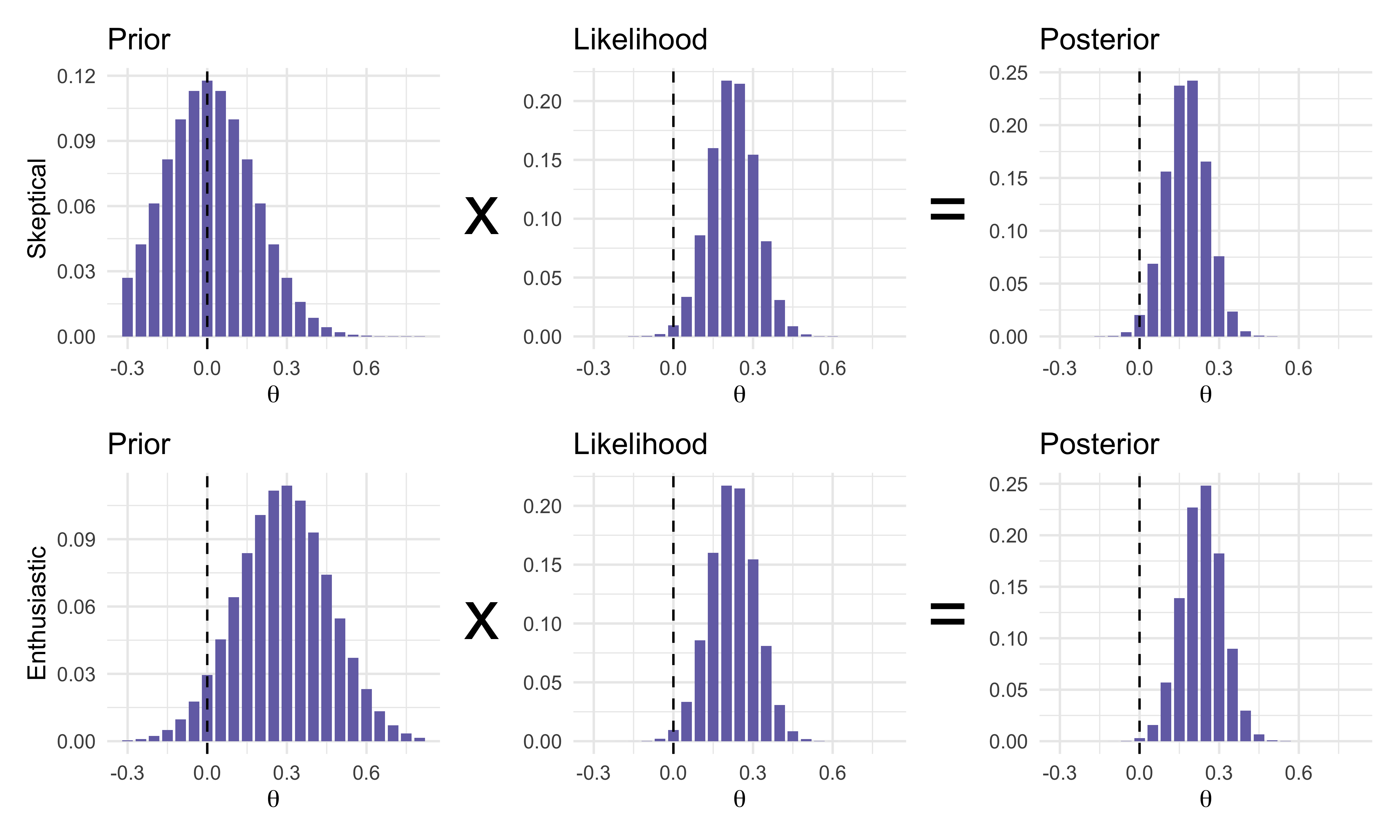
Figure 8.1 shows the mechanism on a grid of the treatment effect, before the table gives the numbers. The likelihood is the same in both rows (508 events, \(\hat\theta = 0.223\) with standard error 0.089), and only the prior changes.
Figure 8.1: Prior times likelihood equals posterior on a grid of the log hazard ratio effect theta = -log HR (step 0.05), for 508 events and observed HR 0.80. Top: skeptical prior N(0, 0.175^2). Bottom: enthusiastic prior N(0.288, 0.175^2). The dashed line marks no effect.
Reading the figure from left to right, the likelihood is identical in the two rows and sits near 0.22, with a spread much narrower than either prior. The skeptical posterior is pulled toward zero and the enthusiastic posterior toward the design effect, but both end up close to the likelihood, because the data carry about four times the weight of either prior. The posterior probability of benefit, \(\Pr(\theta > 0 \mid y)\), is 0.988 under the skeptical prior and 0.999 under the enthusiastic one (exact normal calculation, not the grid sum). The prior moves the posterior, and in this trial it moves the conclusion very little.
Table 8.2: Posterior for a trial with 508 events and observed HR 0.80, under three reference priors. Pr(theta > 0) is the posterior probability of any benefit. ESS is the prior’s weight in events.
Prior
ESS (events)
Posterior median HR
95% interval for HR
Pr(theta > 0)
Noninformative N(0, 100^2)
0
0.800
0.67 to 0.95
0.9940
Skeptical N(0, 0.175^2)
131
0.837
0.72 to 0.98
0.9875
Enthusiastic N(0.288, 0.175^2)
131
0.789
0.68 to 0.92
0.9986
The posterior probability of benefit under the noninformative prior is 0.994, which is one minus the one-sided p-value of 0.006 (the agreement between the traditional and the flat-prior Bayesian answer that Chapter 7 emphasized). The skeptic, who started with only a 5 percent chance that the drug works as designed, ends with a posterior probability of 0.988 that it does something, and a posterior hazard ratio of 0.84. The skeptical prior shrinks the estimate by about a fifth of the way back toward the null, and the evidence is still above 0.975. In this trial the conclusion does not depend on who is asked.
Two warnings apply to this table. The skeptical prior here is not weak: it is worth 131 events, a quarter of the trial. The mean is zero by construction, and the spread is tied to the sponsor’s own design alternative, so a sponsor with an optimistic alternative has a correspondingly wide skeptic. A regulator who thinks the realistic effect is smaller than the design alternative would ask for a different skeptic, centered at the same value with a smaller spread, and the fair response is the sensitivity analysis of the next sections and not an argument about whose skeptic is right. The EOLIA trial is the standard real example of how far a skeptic and an enthusiast can sit from each other on one dataset (88 percent against 99 percent posterior probability of benefit; Section 8.13).
8.4 Why default flat priors fail on the scale that matters
The noninformative prior in the table was harmless because the likelihood for \(\theta\) was normal and the prior was flat on the same scale. It is not harmless in general, and the cases in which it fails are the ones in which a sponsor most needs the prior to behave: small trials, binary endpoints, regression models, and dose-response. The difficulty is that “noninformative” is a statement about one parameterization. A prior that is vague on a parameter is generally informative about every nonlinear function of it, and the treatment effect a trial is designed to estimate is nearly always a function of the parameters. The fullest statement is in the Statistics in Medicine manuscript on priors and predictive stopping (Polson and Sokolov 2026a), whose treatment of this topic this section follows.
Independent beta priors imply an extreme prior on the risk difference
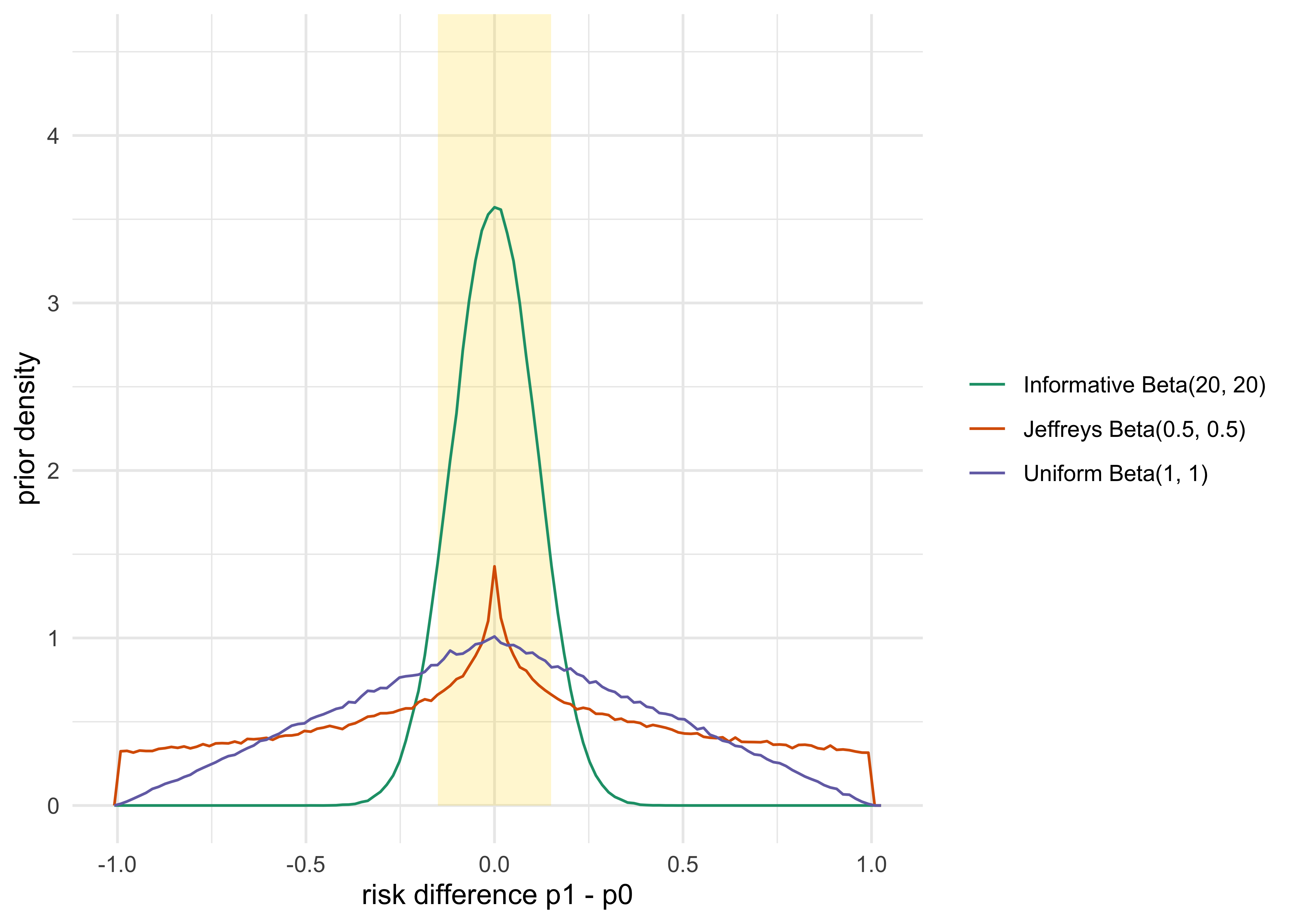
Consider a two-arm trial with a binary endpoint and response rates \(p_1\) (treatment) and \(p_0\) (control). Give each arm a Jeffreys prior (Jeffreys 1946; see Kass and Wasserman 1996 for formal-rule priors), \(\mathrm{Beta}(1/2, 1/2)\), or a uniform prior, \(\mathrm{Beta}(1, 1)\). Each is a respectable noninformative choice for a single proportion. What do they say about the risk difference \(\theta = p_1 - p_0\)? The next chunk (Figure 8.2) answers by simulation and adds a symmetric informative \(\mathrm{Beta}(20, 20)\) for comparison.
Figure 8.2: Implied prior density of the risk difference p1 - p0 under independent priors on the two arms. The shaded band is |delta| <= 0.15, a generic range for illustration and not an indication-specific margin.
Under independent Jeffreys priors, the prior standard deviation of the risk difference is 0.50, and there is a 56 percent prior probability that the two arms differ by more than 30 percentage points. Under independent uniform priors the standard deviation is 0.41 and the same probability is 49 percent. A prior that looks like “no opinion” about each response rate is, about the contrast, the opinion that the drug is very likely either dramatically effective or dramatically harmful. Treatment effects that reach a confirmatory trial are mostly modest (Berry 2012; Sokolova, Sokolov, and Polson 2026), so this is a prior that disagrees with the sponsor’s own experience. These priors permit clinically implausible differences, so their posterior influence and the stopping operating characteristics should be evaluated under the proposed design: with equal arm sizes the posterior mean difference is shrunk toward zero relative to the observed difference, and whether early stops for efficacy are in excess depends on the truth and the monitoring rule.
Beta priors were used in trial analysis by Novick and Grizzle (1965), whose convention reads \(\mathrm{Beta}(z + 1, m - z + 1)\) as \(m\) prior patients with \(z\) responders, the practical way to express a prior in patients, related to the conjugate prior-sample reading of Raiffa and Schlaifer (Raiffa and Schlaifer 1961); Morita, Thall, and Müller (2008) give the general effective sample size. The opposite deliberate choice, a prior that is weak on purpose and a success threshold calibrated by simulation, is the one the BNT162b2 vaccine trial used (Section 8.13).
Flat priors on logistic coefficients
The same issue arises with more force in regression. A logistic dose-response model, \(\mathrm{logit}\, p(x) = \beta_0 + \beta_1 (x - 30)\), has coefficients on the log-odds scale, a scale on which most clinicians have no intuition. The common default is a vague normal prior on each coefficient, for example \(N(0, 10^2)\). The vagueness is an illusion on the probability scale, because the inverse logit saturates: a coefficient on the log-odds scale with standard deviation 10 pushes almost all of the prior mass to the boundaries. Simulating the prior makes the point.
Show the R code
set.seed(2026); b0 <-rnorm(2e5, 0, 10); p_mid <-plogis(b0) # centre of the dose range, where x - 30 = 0extreme <-mean(p_mid <0.05| p_mid >0.95); flat_pct <-round(100* extreme)
For a patient at the center of the dose range, about 77 percent of the prior mass on the response probability lies below 0.05 or above 0.95. The prior says that the drug at that dose either almost always works or almost never does, which is not the “no information” the investigator meant. Sensible diffuse priors on the coefficient scale exist (the familiar recommendation of Gelman and colleagues (Gelman et al. 2008) is a Cauchy prior with scale 2.5 on coefficients of covariates standardized as they describe), but they are a decision to be defended with the same rigor as any other, and the correct way to defend it is to show what it implies on a scale the clinician understands. That is the idea of the next section.
8.5 The conditional means prior
Bedrick, Christensen and Johnson (1996) proposed to move the elicitation from the coefficient scale to the scale where beliefs already exist. The investigator specifies prior distributions for the response probability at several covariate values (dose levels, say), and the prior on the regression coefficients is whatever distribution those statements induce through the link function. A clinician cannot say what the log-odds slope of the dose-response curve is. She can say what she expects at 10 mg and at 50 mg.
For a model with \(p\) coefficients, take \(p\) covariate vectors \(\tilde x_1, \dots, \tilde x_p\) that are linearly independent, so that the map from coefficients to the success probabilities at those points is invertible. Specify independent beta priors, \(\tilde m_i \sim \mathrm{Beta}(a_{1i}, a_{2i})\), for the success probabilities \(\tilde m_i = F(\tilde x_i' \beta)\), where \(F\) is the inverse link. The induced prior on the coefficients is
NoteTechnical note: why the conditional means prior is a data-augmentation prior
Each factor in Equation 8.2 has the form of a binomial likelihood contribution for the success probability at the design point \(\tilde x_i\), with \(a_{1i} - 1\) successes and \(a_{2i} - 1\) failures. The conditional means prior is therefore equivalent to adding \(a_{1i} + a_{2i} - 2\) pseudo-observations at each of the \(p\) design points to the data, with the factor \(f(\tilde x_i'\beta)\) playing the part of the Jacobian of the transformation from probabilities to coefficients. For the logistic link \(f = F(1 - F)\), so the factors combine to \(F^{a_{1i}}(1 - F)^{a_{2i}}\), which is exactly the likelihood of \(a_{1i}\) successes and \(a_{2i}\) failures. A conditional means prior on a logistic model is thus literally \(a_{1i} + a_{2i}\) pseudo-patients, and its weight in the analysis is countable. This is the property that makes the effective sample size of the next section exact for this prior.
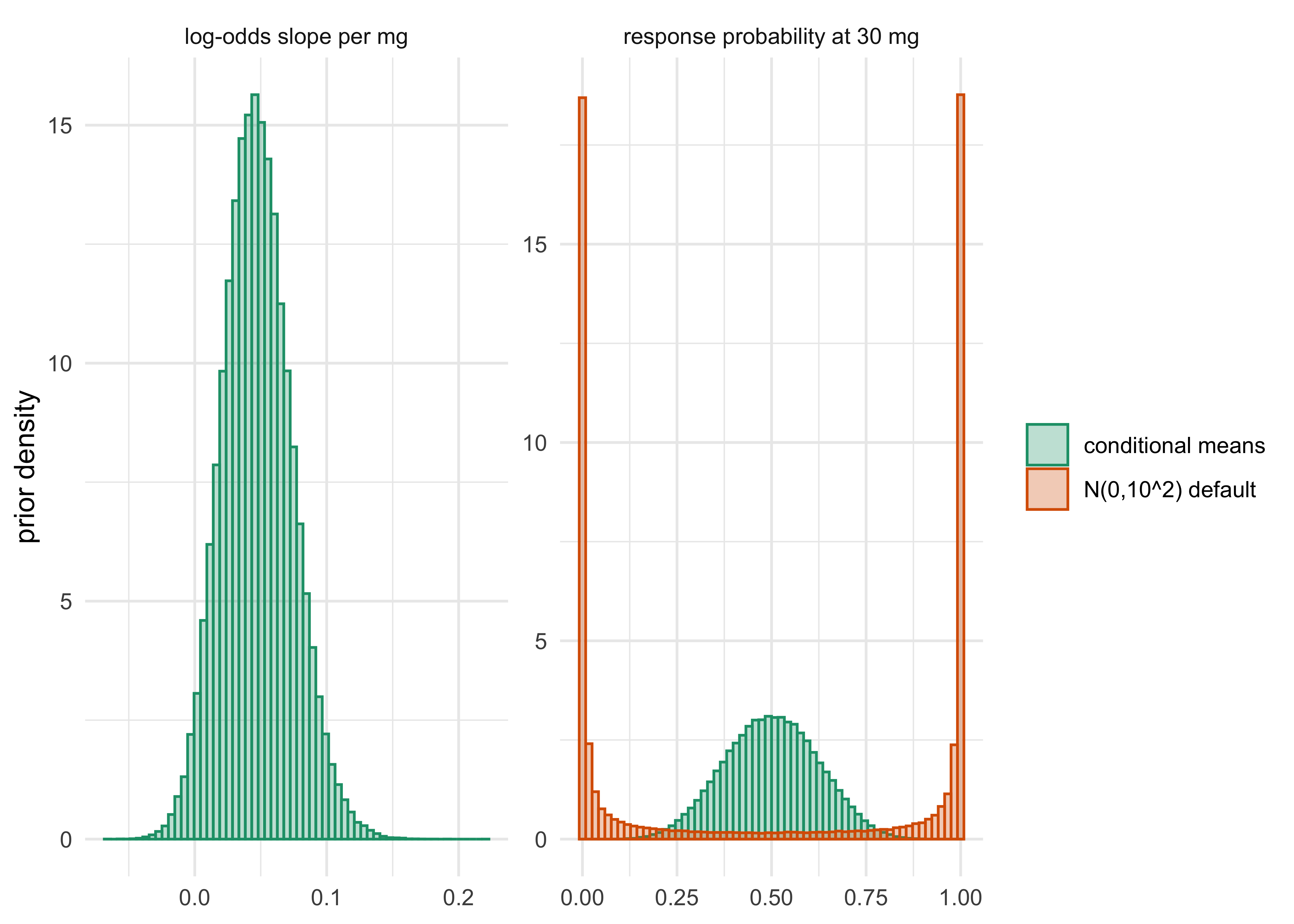
An elicitation that fits in a protocol: the clinician gives for each design point a mean \(m_i\) and a prior sample size \(\nu_i\), and the hyperparameters are \(a_{1i} = \nu_i m_i\) and \(a_{2i} = \nu_i(1 - m_i)\). Suppose the clinician says, for a new agent in a dose range from 10 to 50 mg, that she expects about 30 percent response at 10 mg and 70 percent at 50 mg, with the confidence of 10 patients each. That gives \(\mathrm{Beta}(3, 7)\) at 10 mg and \(\mathrm{Beta}(7, 3)\) at 50 mg. (This example is a numerical illustration, not an indication-specific elicitation.) The chunk below (Figure 8.3) samples from the induced prior and compares it with the default \(N(0, 10^2)\).
Show the R code
cmp <-cmp_samples(3, 7, 7, 3, 10, 50, 2e5, seed =2026)dd <-rbind(data.frame(panel ="response probability at 30 mg", x =plogis(cmp$b0), prior ="conditional means"),data.frame(panel ="response probability at 30 mg", x =plogis(b0), prior ="N(0,10^2) default"),data.frame(panel ="log-odds slope per mg", x = cmp$slope, prior ="conditional means"))ggplot(dd, aes(x, colour = prior, fill = prior)) +geom_histogram(aes(y =after_stat(density)), bins =60, position ="identity", alpha = .3) +facet_wrap(~ panel, scales ="free") +scale_colour_brewer(palette ="Dark2") +scale_fill_brewer(palette ="Dark2") +labs(x =NULL, y ="prior density", colour =NULL, fill =NULL) +theme_minimal()
Figure 8.3: Conditional means prior for a logistic dose-response model with dose centered at 30 mg. Left: induced prior on the response probability at 30 mg, under the elicited Beta(3,7) at 10 mg and Beta(7,3) at 50 mg and under the default N(0, 10^2) coefficients. Right: induced prior on the log-odds slope per mg.
The elicited prior concentrates the response probability at the middle dose near one half and gives the slope a positive mean of 0.047 per mg, with a prior probability of only 3 percent that the slope is negative. The default prior puts nearly all of its mass at the extremes. Two features of this construction help in a protocol. First, the investigator can vary the means to test sensitivity to location, and the sample sizes \(\nu_i\) to test sensitivity to the amount of information, each in units he understands. Second, the induced prior differs between logit and probit links, which means that the same scientific belief gives different coefficient priors for different links without the investigator reasoning about the model (Bedrick, Christensen, and Johnson 1996). One limit is worth recording: independent beta statements at two doses do not enforce a monotone dose-response; if monotonicity is scientifically required, the elicitation must constrain the ordered probabilities or the induced slope. The slope probability reported above (3 percent negative) is the prior’s residual tolerance for a non-monotone response, and it is worth showing to the clinician.
The method is not confined to dose-response models. With a covariate such as baseline severity, the design points are the typical patients at which a clinician has expectations (a mild and a severe patient, in a model with intercept and severity), and the same construction applies. Hanson, Branscum and Johnson (2014) extended the idea through informative \(g\)-priors for logistic regression.
8.6 How much does a prior weigh: effective sample size
A skeptical prior in the previous table was said to be worth 131 events. The idea that a prior has a weight in patients is old (it is the content of the Beta\((z+1, m-z+1)\) parameterization), and Morita, Thall and Müller (2008) made it precise. They define the effective sample size (ESS) of a parametric prior as the number of observations whose information about the parameter is equivalent to the prior’s, using a minimally informative reference prior as the baseline. The practical content for the common models is simple.
For a response probability with a \(\mathrm{Beta}(a, b)\) prior the answer is the one Section 6.4 reached from the weighted-average form of the posterior mean, and the other definitions roughly agree with it:
\[
\mathrm{ESS} = a + b.
\tag{8.3}\]
(The older convention of Novick and Grizzle, under which \(\mathrm{Beta}(z + 1, m - z + 1)\) stands for \(m = a + b - 2\) patients and a uniform prior is worth none, is discussed in Section 6.3; it differs by a constant 2, irrelevant for a prior worth 50 patients and not for one worth 3.) For a normal prior \(\theta \sim N(\mu_0, s_0^2)\) on the mean of observations with variance \(\sigma^2\) per observation,
For the log hazard ratio with 1:1 allocation, each event carries variance 4, so \(\mathrm{ESS} = 4/s_0^2\) events, which is the package function ess_events used above. A skeptical prior with \(s_0 = 0.175\) is worth \(4/0.0306 = 131\) events, and the enthusiastic prior with the same spread is worth the same. If the trial plans 508 events, these priors carry about 26 percent as much information as the data.
The working paper comparing Bayesian and standard design puts the guidance in a sentence: “A prior worth five patients in a trial of five hundred is a modelling choice; a prior worth two hundred is an assumption that needs defending.” (Polson and Sokolov 2026b) The point of reporting ESS is to turn the argument about the prior into an argument about patients. A reviewer may or may not accept that a phase 2 trial of 100 events deserves to count for 50 events in the confirmatory analysis, but both sides can see what they are disagreeing about.
The conditional means prior of the previous section gives a prior ESS of \(\nu_i\) at each design point, here 10 at each of two doses. A power prior on an external dataset of \(n_0\) patients, discounted by a factor \(a_0\) between 0 and 1, has an ESS of about \(a_0 n_0\) (plus the baseline prior’s own weight). Table 8.3 shows the pattern for a phase 2 trial of 100 patients with 30 responders, discounted at four levels; Chapter 19 returns to how \(a_0\) is chosen.
Show the R code
a0 <-c(1, 0.5, 0.25, 0.10); a <-1+ a0 *30; b <-1+ a0 *70knitr::kable(data.frame(a0 =sprintf("%.2f", a0), Prior =sprintf("Beta(%.1f, %.1f)", a, b), `Prior mean`=round(a / (a + b), 3), `ESS = a + b`=round(ess_beta(a, b)), `Share of a 400-patient trial`=sprintf("%.0f%%", 100*ess_beta(a, b) /400), check.names =FALSE))
Table 8.3: A phase 2 result (30 responders of 100) discounted by a power-prior factor a0, as a Beta prior for the control or treatment response rate. Beta(1,1) is the baseline.
a0
Prior
Prior mean
ESS = a + b
Share of a 400-patient trial
1.00
Beta(31.0, 71.0)
0.304
102
26%
0.50
Beta(16.0, 36.0)
0.308
52
13%
0.25
Beta(8.5, 18.5)
0.315
27
7%
0.10
Beta(4.0, 8.0)
0.333
12
3%
Three cautions. First, the formulas give the ESS of a prior in the model’s own information currency, and they are exact for the conjugate beta and normal families. For a mixture prior, such as the robust prior of the next section, the ESS depends on what the data do, because the mixture weights move. The FDA draft recognizes this by asking sponsors to report the ESS “for the entire plausible range of outcomes”, together with its maximum and its mean (Section V.E), and to compare it with the ESS of a noninformative prior. Second, ESS is a summary of the prior’s variance, not its location, so two priors with the same ESS and different means have very different effects on a trial whose truth sits away from the prior mean. Third, a prior can be small in ESS and still decisive: if the trial is at a decision boundary, a prior worth five patients can change the decision. This is why ESS is reported alongside a sensitivity analysis and not instead of one.
The evaluation should also report how the posterior and the operating characteristics change with the prior’s weight (Morita, Thall, and Müller 2010). That is what the next two sections do.
8.7 Prior-data conflict and robust priors
Suppose the prior is informative and well justified, and the data turn out to disagree with it. A fully Bayesian analysis with a single normal prior will compromise between the two, weighted by their precisions, and it will do so however far apart they are. A skeptical prior with a standard deviation of 0.175 will drag a very large observed effect back toward the null by a fixed fraction, and an enthusiastic prior will drag an observed null result toward benefit. For a prior based on external information, such as a phase 2 trial or an earlier study in adults, the same arithmetic says that the posterior is pulled toward information that the data are telling us is irrelevant. The FDA draft recommends that sponsors examine prior-data conflict (Section V.D) and not assume it away.
The standard defense, which this chapter only previews (Chapter 19 develops it, with its connection to power priors and hierarchical models), is a robust mixture prior. The informative component is combined with a weakly informative component, with a prior weight on each. For example, the prior is \(0.8\, N(0.29, 0.10^2) + 0.2\, N(0, 1)\): an 80 percent chance that the effect looks like the phase 2 estimate, and a 20 percent chance that nothing is known. After the data, the weights update: the component that predicted the data better gains weight. If the data agree with the informative component, the posterior stays with it, and if they disagree, the weight shifts to the vague component and the posterior follows the data. Schmidli and colleagues (2014) developed this construction for historical controls, and it is the form the FDA draft calls a mixture prior. The FDA applied it in a real submission, the pediatric belimumab trial in lupus (Section 8.13).
Show the R code
comps <-data.frame(weight =c(0.8, 0.2), mean =c(0.29, 0), sd =c(0.10, 1))mix <-do.call(rbind, lapply(c(0.29, 0.15, 0, -0.20), function(e) { m <-mixture_posterior(e, 0.12, comps); i <-normal_update(0.29, 0.10, e, 0.12)data.frame(`Observed estimate`=sprintf("%+.2f", e), HR =round(exp(-e), 2), `Weight on informative`=round(m$weights[1], 2),`Mixture posterior mean`=sprintf("%+.3f", sum(m$weights * m$means)), `Informative only posterior mean`=sprintf("%+.3f", i$mean),`Pr(theta > 0), mixture`=round(m$p_pos, 3), `Pr(theta > 0), informative only`=round(pnorm(i$mean / i$sd), 3), check.names =FALSE) }))knitr::kable(mix)
Table 8.4: Robust mixture prior 0.8 N(0.29, 0.10^2) + 0.2 N(0, 1^2) against the pure informative prior N(0.29, 0.10^2), for four observed log hazard ratio estimates with standard error 0.12. Weight is the posterior weight of the informative component.
Observed estimate
HR
Weight on informative
Mixture posterior mean
Informative only posterior mean
Pr(theta > 0), mixture
Pr(theta > 0), informative only
+0.29
0.75
0.96
+0.290
+0.290
1.000
1.000
+0.15
0.86
0.95
+0.228
+0.233
0.993
0.999
+0.00
1.00
0.82
+0.141
+0.171
0.900
0.987
-0.20
1.22
0.16
-0.151
+0.089
0.182
0.877
In Table 8.4, when the observed effect equals the informative mean, the mixture and the single prior agree and the informative component keeps 96 percent of its weight. When the observed log hazard ratio is \(-0.20\), a harmful effect of a hazard ratio of 1.22 that lies about three prior-predictive standard deviations from the informative prior’s center, the pure informative prior still reports a positive posterior mean of 0.089 (the data pull it only part of the way, and it gives a posterior probability of benefit of 0.88), while the mixture has moved 84 percent of its weight to the vague component and reports a posterior mean of -0.151, much closer to the data, with a posterior probability of benefit of 0.18. The mixture is, in effect, a prior that has an opinion about what would count as disagreement, which a single normal cannot have. That is what the regulator has in mind when it asks whether the method will “borrow less when the data are less similar” (the draft’s description of dynamic discounting methods, Section V.D).
The robust prior has a price. The weight 0.2 on the vague component is itself a prior judgment, and the operating characteristics (type I error when the informative prior is wrong, and the extra patients needed to detect it) have to be simulated. The simulation is the business of Chapter 14, and the justification of the informative component, which is the part a regulator will contest, is the business of Chapter 19.
8.8 Sensitivity analysis over the prior scale
The FDA draft asks that “sensitivity analyses should be planned that utilize a range of alternative reasonable choices for the prior distributions” (Section V.F), for instance by varying the strength of borrowing. The working paper comparing Bayesian and standard design says that it reports a sensitivity analysis for every Bayesian number (Polson and Sokolov 2026b), and the protocol table calls for “a prespecified sensitivity analysis over the prior scale”. For a normal prior the natural one-parameter family is the prior standard deviation \(s_0\) at a fixed mean, because \(s_0\) sets the ESS through Equation 8.4 and spans the range from a dogmatic prior (\(s_0 \to 0\)) to a noninformative one (\(s_0 \to \infty\)).
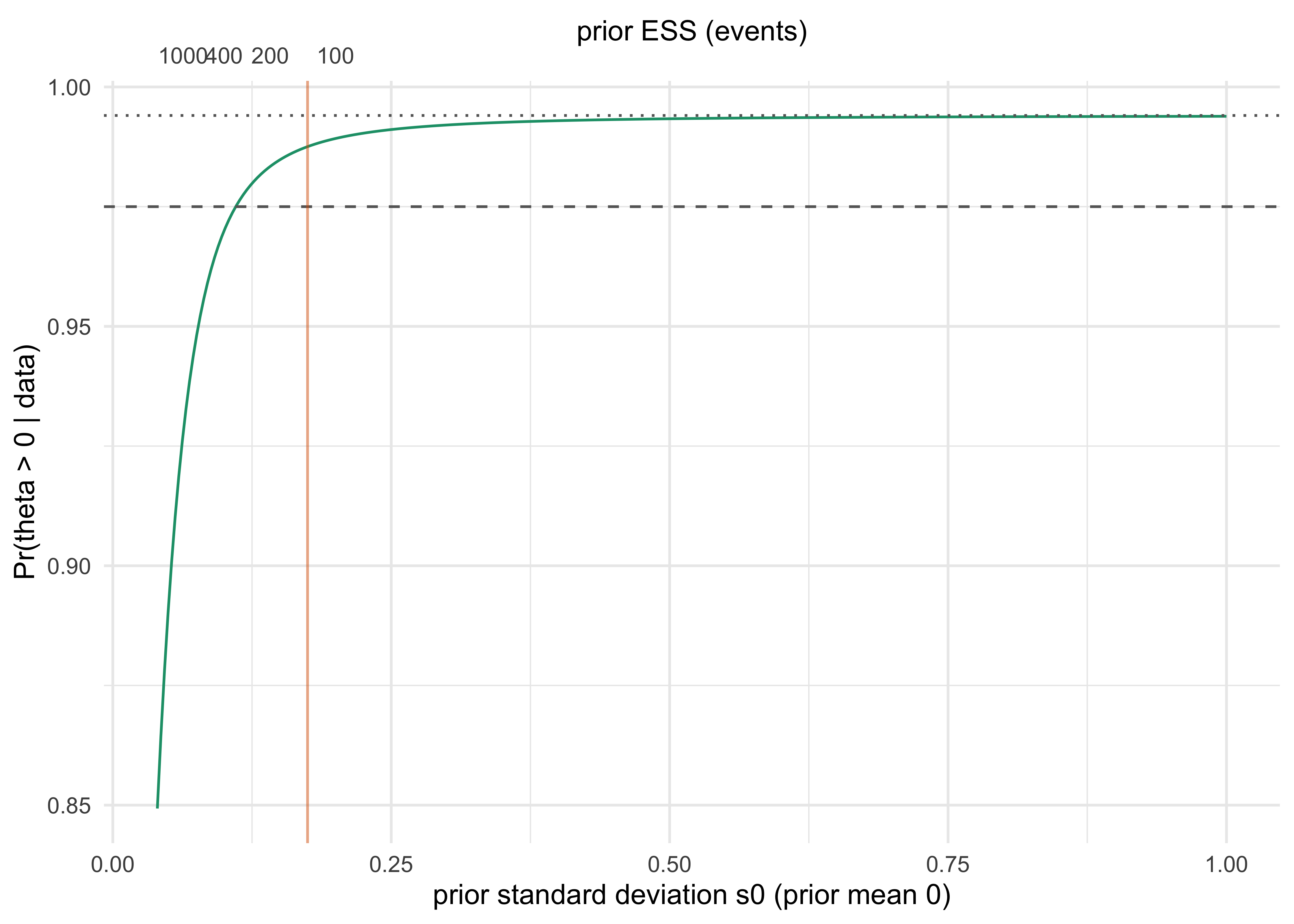
Figure 8.4: Posterior probability of benefit Pr(theta > 0 | data) for the 508-event trial with observed HR 0.80, as the standard deviation of a prior centered at zero (the skeptical family) varies. The upper axis gives the corresponding prior ESS in events. The dashed line is the 0.975 threshold.
The curve in Figure 8.4 is flat to the right and falls only when the prior becomes strong. For prior standard deviations above about 0.15 (ESS up to about 180 events) the posterior probability of benefit stays above 0.98; it falls below the 0.975 threshold only when the skeptical prior is as tight as \(s_0 = 0.11\), which is worth 328 events, about two thirds of the information in the trial. This shape is the typical answer when the data are decisive: the conclusion is robust to a wide family of priors and breaks only for priors that are themselves almost as informative as the trial. The multiplatform heparin trials pre-specified an enthusiastic prior as exactly this kind of check (Section 8.13).
The tipping-point prior
The sensitivity curve suggests a sharper way of reporting, borrowed from the handling of missing data: instead of asking what the conclusion is under a given prior, ask which prior would reverse it. A tipping-point prior is the least extreme prior in a stated family for which the success criterion is no longer met. In the family above, the tipping point is a standard deviation of 0.11, or an ESS of 328 events. A second family varies the prior mean at a fixed spread, which asks how pessimistic the skeptic must be to overturn the result. Holding the skeptical spread of 0.175, the posterior probability of benefit drops below 0.975 only if the prior mean is -0.109, a prior expectation of a hazard ratio of 1.12, which is to say a skeptic who believed that the drug was harmful on average before seeing the data.
The tipping-point report is useful to the regulator because it replaces a debate about the right prior with a statement about which priors the regulator would have to hold to disagree with the sponsor, and a regulator can say plainly whether she holds one. A tipping point that lies in an incredible region (a skeptic who thought the drug harmful, a prior worth two thirds of the trial) supports the claim that the conclusion is driven by the data. A tipping point close to the sponsor’s own prior is a warning that the prior drives the answer, which is the case that point 6 of the next section addresses.
The tipping-point analysis belongs in the statistical analysis plan, with the family and the success criterion written down before unblinding; a family chosen after seeing the data would be a way of looking for a prior that works.
8.9 What the FDA draft says
The FDA’s January 2026 draft guidance is the first FDA statement on the Bayesian method in drug trials in general, and its position on priors can be stated in six points. The text of the draft governs; the points below are a summary of Section IV.B and the section on priors.
Pre-specification. “It is always critical for Bayesian analyses to have a prespecified prior” (Section IV.B), and the sponsor should pre-specify and justify the full details of the prior in the protocol. The prior used for analysis (the analysis prior) is distinguished from design (sampling) priors used only in planning simulations; the second may be skeptical or optimistic about the truth to explore performance, but only the first enters the inference.
Calibration or direct use of the posterior. The draft describes three routes for the success criterion \(\Pr(\delta > a \mid \text{data}) > c\): calibration to type I error, direct interpretation of posterior probabilities, and benefit-risk or decision-theoretic criteria. In a calibrated design, \(a\) and \(c\) are chosen by simulation so that the familywise type I error is at most 0.025 one-sided, and the prior is used as a modeling device whose choice affects power and not the error rate. In a non-calibrated design, in which the prior is meant to summarize real external information, the posterior probability is read directly (a posterior probability of 0.98 means a 2 percent probability of ineffectiveness given the prior), and this is acceptable where the prior is specified so that it “accurately and comprehensively reflects the external data” (Section IV.A), by agreement with the Agency. Here the prior matters in the second sense: without calibration, “the accuracy of conclusions depends strongly on the choice of prior distribution” (Section IV.B.2). The third, decision-theoretic route chooses the threshold from stated losses (Section 1.6). The calibration route is the subject of Chapter 14.
Noninformative and minimally informative priors. No single approach is universally preferred. They can still influence the posterior when data are sparse, and they are not invariant to transformation, so a prior that is flat on one scale must be checked on the scale of the estimand: the point of the beta and logistic examples above. They also serve as the reference against which ESS is reported.
Skeptical priors. “Skeptical priors express skepticism about the presence of very large treatment effects.” They may be appropriate after failed related programs or where only an incremental gain is plausible, and they can stand in for adjusting an early-stopping boundary. The same section also discusses enthusiastic priors.
Informative priors need more. “Informative priors will generally need a greater amount of justification” (Section V.A), with strong justification for borrowing on the grounds of relevance and feasibility, most commonly in pediatrics and rare diseases. Details of prior construction (a pre-specified search, criteria against preferential selection of favorable studies, relevance of the estimand and population) are the substance of Chapter 19.
Quantify the influence. Report the prior mean and the ESS, over the plausible range of outcomes, and plan sensitivity analyses over alternative reasonable priors. The “when the prior drives the answer” scenario is the one in which a sponsor must show, by the sensitivity curve and the tipping point, that the conclusion survives or must justify the prior at the level of evidence that a regulator accepts for any other analytic assumption.
The draft leaves several things open. It does not say how large an ESS is acceptable, how wide a family of sensitivity priors is enough, or how to resolve a disagreement between a sponsor’s prior and the Agency’s. These are the points on which a sponsor should seek agreement in a formal meeting before the trial (the programs are in Chapter 3 and the practicalities in Chapter 23). The draft is also not binding, and a sponsor who relies on it should say in the briefing document that it does.
ICH E20 in its Step 2 draft treats the prior in the same spirit, in Section 5.3: the Bayesian analysis combines a prior with the trial data, within the draft’s general expectation that adaptations and analysis methods are pre-specified and that the design’s performance is evaluated by simulation (see Chapter 14). As a Step 2 text, E20 was open for public consultation until 30 November 2025 and may change before final adoption.
The device precedent
None of this is new at the Agency. The Center for Devices and Radiological Health issued its Bayesian guidance for medical device trials as a draft in 2006 and in final form in February 2010 (U.S. Food and Drug Administration 2010), and several device approvals have rested on priors built from earlier studies, often a previous generation of the same device. The device guidance’s recipe is the one this chapter describes in different words: agree on the prior with the Agency before the trial, justify the exchangeability of the earlier data with the current trial, quantify how much the earlier data count, and show by simulation how the design performs when the prior is wrong. On the type I error it says (Section 4.8, “Assessing the operating characteristics of a Bayesian design”): “When using prior information, it may be appropriate to control type I error at a less stringent level than when no prior information is used,” and the degree of relaxation “is a case-by-case decision that depends on many factors, primarily the confidence we have in the prior information.” This parallels the distinction the 2026 drug draft draws between calibrated and non-calibrated designs. The device precedent shows that the regulatory machinery for an informative prior exists and works, and it shows the limits: devices are often iterations of a platform with a plausible exchangeability argument, an argument that is much harder for a new molecular entity.
8.10 Side by side: what changes in the protocol
Item
Traditional design
Bayesian design
Prior information
Implicit in the design alternative and the assumed variance or event rate
Stated as a distribution, with source and justification
Where the sponsor’s uncertainty appears
Nowhere in the analysis; sometimes in an assurance calculation
In the prior and in the sensitivity analysis
How the effect of the assumption is reported
Power at several alternatives
Prior ESS; posterior under a skeptical, enthusiastic and noninformative prior; tipping point
Agreement with the regulator
Design alternative and sample size
Prior, success criterion, calibration, and sensitivity family
When the traditional and Bayesian answers agree
Flat prior and a normal likelihood: Pr(effect > 0) equals one minus the one-sided p-value
Main regulatory question
“Is the assumed effect realistic?”
“Why this prior, how much does it weigh, and does it drive the answer?”
What stays the same is the standard of evidence: the trial is still judged by whether the conclusion would survive an informed skeptic, and a Bayesian design for a confirmatory trial is calibrated to the same one-sided 0.025 when the prior is not meant to carry information. What changes is that the assumptions are written down and can be argued with.
8.11 Writing the prior into the protocol
TipIn the protocol
A prior section of a protocol or statistical analysis plan should contain, at minimum:
The analysis prior, by name and parameters, on the scale of the estimand, together with its implied distribution for the estimand (for example, the implied prior on the risk difference or the hazard ratio) so that a reviewer does not have to compute it.
Its provenance: the data, search or elicitation exercise from which it was built, with the dates and the people involved, and the criteria for including or excluding sources, written before the data from the current trial are seen.
Its effective sample size, as defined in Morita, Thall and Müller (2008), by formula for conjugate priors and by simulation for mixtures, over the plausible range of outcomes, and as a share of the planned sample size.
The comparison priors: a noninformative prior (reference), a skeptical prior, and where useful an enthusiastic prior, with the posterior summaries under each.
The sensitivity analysis: the family of priors (for example, standard deviation from the ESS-zero reference to twice the proposed ESS; mean over a stated range), the success criterion, and the tipping-point report.
The robustness provision: if the prior is informative, the mixture or discounting rule applied under prior-data conflict, with its parameters, and the simulation that evaluated it.
The success criterion and its calibration: whether \(a\) and \(c\) are calibrated to a familywise type I error of 0.025 one-sided by simulation, or the posterior probability is to be read directly (with the agreement with the Agency that supports it), or a benefit-risk or decision-theoretic criterion is used, with its losses.
8.12 What can go wrong
Four failures recur, and a sponsor can guard against each.
The prior chosen after the data are seen. A prior that is fixed after unblinding is a free parameter, and an analysis plan that allows it is a plan that allows the conclusion to be selected. Pre-specification is not a formality (the first quotation in the regulatory anchor says “always critical”), and the sensitivity family and the tipping-point report are fixed in the same document.
A single published estimate treated as a prior. One phase 2 result, selected for a good look, is the case simulated above. The cure is to discount, to center on a population of programs and not on the sponsor’s own estimate, or to cap the prior’s ESS at a level the sponsor is willing to defend.
A flat prior mistaken for no prior. A flat prior is a choice and one that carries implicit commitments on every other scale. Compute what it implies about the estimand before claiming that it is neutral. In a large trial with a normal likelihood the issue disappears, and for small binary trials, dose-response and subgroup models it does not.
A prior that matters presented as a prior that does not. A skeptical prior of ESS 131 in a trial of 508 events changes the posterior hazard ratio from 0.80 to 0.84. That is a prior that matters to the estimate, even if the conclusion survives. The report should say so, and let the reader judge.
8.13 In practice
Four trials show the prior at work: one where the regulator asked for a tipping-point analysis, one family of platform trials that fixed neutral priors in advance and tested an enthusiastic one, one reanalysis that shows the prior moving the conclusion, and one pivotal trial that chose a deliberately weak prior.
Pediatric belimumab in lupus: a tipping point over the borrowing weight
The pediatric trial of intravenous belimumab in lupus (C1109, PLUTO) was not powered to stand on its own, so FDA requested a post hoc analysis that borrowed from the adult trials through a robust mixture prior with borrowing weight \(w\)(Brunner et al. 2020; U.S. Food and Drug Administration, Center for Drug Evaluation and Research 2026). The sponsor was not asked to defend a single \(w\): the posterior probability of efficacy was at least 97.5 percent whenever \(w\) was 0.55 or more, and the review division judged such a weight reasonable (Pottackal et al. 2025). The data, the mixture and the approval are told in Section 19.17.2.
The lesson is the tipping-point logic of Section 8.8.1 applied to the borrowing weight instead of the prior spread: the report names the weakest reliance on adult data under which the conclusion holds, and the argument moves from “what is the right weight” to “is a weight of 0.55 or more credible”. The FDA case study also stresses that the analysis was post hoc, and recommends that a future program agree and pre-specify the Bayesian approach early (pre-IND), which is the point of the regulatory anchor of this chapter. Chapter 19 returns to the mixture itself.
REMAP-CAP and the multiplatform heparin trials: neutral priors, enthusiastic sensitivity
The REMAP-CAP platform fitted a Bayesian cumulative logistic model for organ support-free days, with neutral prior distributions for the individual treatment effects, and fixed its efficacy threshold (a posterior probability of an odds ratio above 1 exceeding 99 percent) before the data (REMAP-CAP Investigators, Gordon, et al. 2021). The tocilizumab results are in Section 6.12. The point here is the choice of prior: it favored neither arm, so that the data had to do the work.
The therapeutic heparin trials (ATTACC, ACTIV-4a and REMAP-CAP, run as a multiplatform trial) used the same style: weakly informative priors for the baseline probabilities, a hierarchical prior with the severe and moderate cohorts nested around an overall effect with a neutral mean, superiority at a posterior probability above 99 percent and futility at above 95 percent for an odds ratio below 1.2. The pre-specified sensitivity analysis used an enthusiastic prior with a mean odds ratio of 1.75 (95 percent credible interval 0.74 to 4.15, prior probability of superiority 90 percent), the enthusiastic reference prior of this chapter (REMAP-CAP Investigators, ACTIV-4a Investigators, et al. 2021; ATTACC Investigators et al. 2021). Enrollment in critically ill patients stopped for futility (adjusted odds ratio 0.83, 95 percent credible interval 0.67 to 1.03), and in non-critically ill patients the neutral-prior analysis gave a 98.6 percent posterior probability that therapeutic dosing increased organ support-free days (odds ratio 1.27, 1.03 to 1.58) (ATTACC Investigators et al. 2021).
The lesson is the structure and not a single number. Neutral analysis priors, a calibration of the thresholds by simulation, and an enthusiastic prior as a stress test: a conclusion that holds with a skeptical-to-neutral analysis prior and is not overturned by the optimist is hard to attack. Chapter 20 treats the platform designs themselves.
EOLIA: how far the prior moves the conclusion
EOLIA, whose design and p-value of 0.09 are described in Section 7.10 and whose full reanalysis is in Section 22.3, is the standard real example of how far the prior can move a conclusion. In the post hoc reanalysis (Goligher et al. 2018) the posterior probability of any mortality benefit ranged from 88 percent under a strongly skeptical prior to 99 percent under an enthusiastic or a published-study prior.
The same reanalysis shows what the prior does not change. The probability that the absolute risk reduction reached the 20 points the trial was designed to detect stayed small under every prior (see Section 22.3). The lesson is the one of the sensitivity curve of this chapter: report the posterior probability of the clinically relevant effect (and not only of any benefit) under a skeptical, a neutral and an enthusiastic prior, and read the range, not a single value. The range 88 to 99 percent says that the answer about “some benefit” depends on who is asked, and the small probability of the large benefit says that the trial was not built for the effect size it assumed.
BNT162b2: a deliberately weak prior with a calibrated threshold
The pivotal Pfizer-BioNTech vaccine trial (analysis and numbers in Section 6.12) made the opposite choice: a deliberately weak prior with a threshold calibrated by simulation. Its \(\mathrm{Beta}(0.700102, 1)\) prior on \(p = (1 - \mathrm{VE})/(2 - \mathrm{VE})\), the probability that a case falls in the vaccine arm, has mean 0.4118 (the value at \(\mathrm{VE} = 30\) percent) and an ESS by Equation 8.3 of \(a + b = 1.7\) cases, against a final analysis planned at 164 cases. Success required a posterior probability of \(\mathrm{VE} > 30\) percent above 0.995 at an interim analysis and above 0.986 at the final one, with the thresholds set by simulation so that the overall one-sided type I error was 0.025 (Pfizer Inc. 2022).
The lesson is the calibrated route of the FDA draft (point 2 of Section 8.9): the prior is a modeling device, small enough that no reviewer could say it carried the result, and the evidence standard sits in the threshold, whose frequentist behavior was checked in advance. The posterior calculation for this prior is in Section 6.12.
Key points
The traditional design conditions on a design alternative in the power calculation and states no uncertainty about it. A Bayesian protocol asks the sponsor to state that uncertainty as a prior, and assurance averages power over it.
Priors come from phase 2 data, earlier programs and literature, structured expert elicitation (SHELF) and mechanistic models. Phase 2 estimates are inflated by selection: in the illustration, programs that advanced had a phase 2 hazard ratio of 0.71 and a true one of 0.86.
Skeptical, enthusiastic and noninformative priors are reference points that show which audiences the data convince. A skeptical prior with a 5 percent chance of the design effect is worth 131 events here, a quarter of a 508-event trial.
“Flat” is a statement about one scale. Independent uniform or Jeffreys priors on two arms put 49 to 56 percent prior probability on a risk difference larger than 30 points, and N(0, 10^2) priors on logistic coefficients put 77 percent of mass on probabilities below 0.05 or above 0.95. The conditional means prior moves the elicitation to the probability scale, and it is a data-augmentation prior with countable pseudo-patients.
Effective sample size reports the weight of a prior in patients: \(a + b\) for a beta, \(\sigma^2 / s_0^2\) for a normal, \(4/s_0^2\) events for a log hazard ratio. A prior worth 5 patients in a trial of 500 is a modeling choice and one worth 200 is an assumption.
A robust mixture prior defends against prior-data conflict by moving weight to a vague component when data disagree. It has its own price and is treated in Chapter 19.
Report a sensitivity analysis over the prior scale and a tipping point: the weakest prior in a stated family that reverses the conclusion.
In practice: the belimumab pediatric analysis reported a tipping point over the borrowing weight (efficacy at least 97.5 percent once \(w \geq 0.55\)), the multiplatform heparin trials stress-tested neutral priors with an enthusiastic one, EOLIA’s posterior probability of benefit ranged from 88 to 99 percent with the prior, and BNT162b2 used a Beta(0.700102, 1) prior worth 1.7 cases with calibrated thresholds.
The FDA’s January 2026 draft recommends a pre-specified prior, distinguishes calibrated from non-calibrated success criteria, and asks for the ESS and sensitivity analyses. It is a draft; the 2010 device guidance is the final precedent.
NoteDiscussion questions
Your phase 3 protocol uses a hazard ratio of 0.75 for the sample size. The design alternative is a planning assumption, not a prior. What prior would you actually defend for the hazard ratio, which uncertainty would it carry, and where would that uncertainty come from?
A sponsor proposes to use a phase 2 estimate with a hazard ratio of 0.65 as the center of an informative prior in the confirmatory trial. List three questions you would ask about how the phase 2 result came to be in the program. How would you change the prior, in the light of the selection simulation of this chapter?
A reviewer says that the skeptical prior in your analysis is too weak, and proposes one centered at a hazard ratio of 1.05. How should the tipping-point report be designed so that this conversation can be settled with a number?
For a rare-disease trial of 60 patients, a prior of ESS 20 is proposed from a registry. The posterior probability of benefit is 0.96 under the prior and 0.88 under a noninformative prior. Is the prior driving the answer? What does the FDA draft say about the non-calibrated route, and what would you want to see before agreeing?
Why does the conditional means prior make it easier to check an elicited prior against the clinician’s beliefs than a prior on regression coefficients? Which statements would you ask the clinician to confirm before the protocol is locked?
Abrams, Keith, Deborah Ashby, and Daniel Errington. 1994. “Simple Bayesian Analysis in Clinical Trials: A Tutorial.”Controlled Clinical Trials 15 (5): 349–59. https://doi.org/10.1016/0197-2456(94)90032-9.
ATTACC Investigators, ACTIV-4a Investigators, REMAP-CAP Investigators, Patrick R. Lawler, Ewan C. Goligher, Jeffrey S. Berger, et al. 2021. “Therapeutic Anticoagulation with Heparin in Noncritically Ill Patients with Covid-19.”New England Journal of Medicine 385 (9): 790–802. https://doi.org/10.1056/NEJMoa2105911.
Bedrick, Edward J., Ronald Christensen, and Wesley Johnson. 1996. “A New Perspective on Priors for Generalized Linear Models.”Journal of the American Statistical Association 91 (436): 1450–60.
Berger, James. 2006. “The Case for Objective Bayesian Analysis.”Bayesian Analysis 1 (3): 385–402. https://doi.org/10.1214/06-BA115.
Berry, Donald A. 2012. “Adaptive Clinical Trials in Oncology.”Nature Reviews Clinical Oncology 9 (4): 199–207.
Brunner, Hermine I, Carlos Abud-Mendoza, Diego O Viola, Inmaculada Calvo Penades, Deborah Levy, Jordi Anton, Julia E Calderon, et al. 2020. “Safety and Efficacy of Intravenous Belimumab in Children with Systemic Lupus Erythematosus: Results from a Randomised, Placebo-Controlled Trial.”Annals of the Rheumatic Diseases 79 (10): 1340–48. https://doi.org/10.1136/annrheumdis-2020-217101.
Chaloner, Kathryn, Timothy Church, Thomas A. Louis, and John P. Matts. 1993. “Graphical Elicitation of a Prior Distribution for a Clinical Trial.”Journal of the Royal Statistical Society, Series D (The Statistician) 42 (4): 341–53. https://doi.org/10.2307/2348469.
Dallow, Nigel, Nicky Best, and Timothy H. Montague. 2018. “Better Decision Making in Drug Development Through Adoption of Formal Prior Elicitation.”Pharmaceutical Statistics 17 (4): 301–16. https://doi.org/10.1002/pst.1854.
Freedman, L. S., D. Lowe, and P. Macaskill. 1984. “Stopping Rules for Clinical Trials Incorporating Clinical Opinion.”Biometrics 40 (3): 575–86. https://doi.org/10.2307/2530902.
Freedman, L. S., and D. J. Spiegelhalter. 1983. “The Assessment of Subjective Opinion and Its Use in Relation to Stopping Rules for Clinical Trials.”The Statistician 32 (1/2): 153–60. https://doi.org/10.2307/2987606.
Freedman, Laurence S., and David J. Spiegelhalter. 1989. “Comparison of Bayesian with Group Sequential Methods for Monitoring Clinical Trials.”Controlled Clinical Trials 10 (4): 357–67. https://doi.org/10.1016/0197-2456(89)90001-9.
Freedman, Laurence S., David J. Spiegelhalter, and Mahesh K. B. Parmar. 1994. “The What, Why and How of Bayesian Clinical Trials Monitoring.”Statistics in Medicine 13 (13–14): 1371–83.
Garthwaite, Paul H., Joseph B. Kadane, and Anthony O’Hagan. 2005. “Statistical Methods for Eliciting Probability Distributions.”Journal of the American Statistical Association 100 (470): 680–701. https://doi.org/10.1198/016214505000000105.
Gelman, Andrew. 2006. “Prior Distributions for Variance Parameters in Hierarchical Models.”Bayesian Analysis 1 (3): 515–34. https://doi.org/10.1214/06-BA117A.
Gelman, Andrew, Aleks Jakulin, Maria Grazia Pittau, and Yu-Sung Su. 2008. “A Weakly Informative Default Prior Distribution for Logistic and Other Regression Models.”The Annals of Applied Statistics 2 (4): 1360–83. https://doi.org/10.1214/08-AOAS191.
Goligher, Ewan C., George Tomlinson, David Hajage, et al. 2018. “Extracorporeal Membrane Oxygenation for Severe Acute Respiratory Distress Syndrome and Posterior Probability of Mortality Benefit in a Post Hoc Bayesian Analysis of a Randomized Clinical Trial.”JAMA 320 (21): 2251–59.
Gosling, John Paul. 2018. “SHELF: The Sheffield Elicitation Framework.” In Elicitation: The Science and Art of Structuring Judgement, edited by Luis C. Dias, Alec Morton, and John Quigley, 61–93. Springer. https://doi.org/10.1007/978-3-319-65052-4_4.
Hanson, Timothy E., Adam J. Branscum, and Wesley O. Johnson. 2014. “Informative \(g\)-Priors for Logistic Regression.”Bayesian Analysis 9 (3): 597–612.
Jeffreys, Harold. 1946. “An Invariant Form for the Prior Probability in Estimation Problems.”Proceedings of the Royal Society of London. Series A 186 (1007): 453–61. https://doi.org/10.1098/rspa.1946.0056.
Kass, Robert E., and Larry Wasserman. 1996. “The Selection of Prior Distributions by Formal Rules.”Journal of the American Statistical Association 91 (435): 1343–70. https://doi.org/10.1080/01621459.1996.10477003.
Morita, Satoshi, Peter F. Thall, and Peter Müller. 2008. “Determining the Effective Sample Size of a Parametric Prior.”Biometrics 64 (2): 595–602.
Novick, Melvin R., and James E. Grizzle. 1965. “A Bayesian Approach to the Analysis of Data from Clinical Trials.”Journal of the American Statistical Association 60 (309): 81–96.
O’Hagan, Anthony, Caitlin E. Buck, Alireza Daneshkhah, J. Richard Eiser, Paul H. Garthwaite, David J. Jenkinson, Jeremy E. Oakley, and Tim Rakow. 2006. Uncertain Judgements: Eliciting Experts’ Probabilities. Chichester: Wiley. https://doi.org/10.1002/0470033312.
O’Hagan, Anthony, John W. Stevens, and Michael J. Campbell. 2005. “Assurance in Clinical Trial Design.”Pharmaceutical Statistics 4 (3): 187–201. https://doi.org/10.1002/pst.175.
Oakley, Jeremy E., and Anthony O’Hagan. 2019. “SHELF: The Sheffield Elicitation Framework.” School of Mathematics; Statistics, University of Sheffield. http://www.tonyohagan.co.uk/shelf/.
Parmar, Mahesh K. B., Gareth O. Griffiths, David J. Spiegelhalter, Robert L. Souhami, Douglas G. Altman, and Emile van der Scheuren. 2001. “Monitoring of Large Randomised Clinical Trials: A New Approach with Bayesian Methods.”The Lancet 358 (9279): 375–81. https://doi.org/10.1016/S0140-6736(01)05558-1.
Parmar, Mahesh K. B., David J. Spiegelhalter, Laurence S. Freedman, and CHART Steering Committee. 1994. “The CHART Trials: Bayesian Design and Monitoring in Practice.”Statistics in Medicine 13 (13–14): 1297–1312. https://doi.org/10.1002/sim.4780131304.
Polson, Nicholas G., and Vadim Sokolov. 2026a. “Bayesian Adaptive Clinical Trials: Priors, Thompson Sampling, Predictive Stopping and Backward Induction.”
———. 2026b. “Bayesian Versus Standard Clinical Trial Design: Theory, Evidence, and Protocol.”
Pottackal, Ginto, James Travis, Lei Nie, Rebecca Chiu, Rosemarie Neuner, Gregory Levin, Jing Niu, Anshu Marathe, Lily (Yeruk) Mulugeta, and Nikolay P. Nikolov. 2025. “Application of Bayesian Statistics to Support Approval of Intravenous Belimumab in Children with Systemic Lupus Erythematosus in the United States.”Lupus 34 (9): 943–52. https://doi.org/10.1177/09612033251349930.
Raiffa, Howard, and Robert Schlaifer. 1961. Applied Statistical Decision Theory. Boston: Division of Research, Graduate School of Business Administration, Harvard University.
REMAP-CAP Investigators, ACTIV-4a Investigators, ATTACC Investigators, Ewan C. Goligher, Corrinne A. Bradbury, Bryan J. McVerry, et al. 2021. “Therapeutic Anticoagulation with Heparin in Critically Ill Patients with Covid-19.”New England Journal of Medicine 385 (9): 777–89. https://doi.org/10.1056/NEJMoa2103417.
REMAP-CAP Investigators, Anthony C. Gordon, Paul R. Mouncey, Farah Al-Beidh, Kathryn M. Rowan, Alistair D. Nichol, et al. 2021. “Interleukin-6 Receptor Antagonists in Critically Ill Patients with Covid-19.”New England Journal of Medicine 384 (16): 1491–1502. https://doi.org/10.1056/NEJMoa2100433.
Schmidli, Heinz, Sandro Gsteiger, Satrajit Roychoudhury, Anthony O’Hagan, David Spiegelhalter, and Beat Neuenschwander. 2014. “Robust Meta-Analytic-Predictive Priors in Clinical Trials with Historical Control Information.”Biometrics 70 (4): 1023–32. https://doi.org/10.1111/biom.12242.
Simpson, Daniel, Håvard Rue, Andrea Riebler, Thiago G. Martins, and Sigrunn H. Sørbye. 2017. “Penalising Model Component Complexity: A Principled, Practical Approach to Constructing Priors.”Statistical Science 32 (1): 1–28. https://doi.org/10.1214/16-STS576.
Sokolova, Alexandra, Vadim Sokolov, and Nicholas G. Polson. 2026. “Some Bayesian Perspectives on Clinical Trials.”arXiv Preprint arXiv:2602.09208.
Spiegelhalter, David J., Keith R. Abrams, and Jonathan P. Myles. 2004. Bayesian Approaches to Clinical Trials and Health-Care Evaluation. Chichester: Wiley. https://doi.org/10.1002/0470092602.
Spiegelhalter, David J., Laurence S. Freedman, and Mahesh K. B. Parmar. 1994. “Bayesian Approaches to Randomized Trials.”Journal of the Royal Statistical Society, Series A 157 (3): 357–416. https://doi.org/10.2307/2983527.
Spiegelhalter, David J., Jonathan P. Myles, David R. Jones, and Keith R. Abrams. 2000. “Bayesian Methods in Health Technology Assessment: A Review.”Health Technology Assessment 4 (38). https://doi.org/10.3310/hta4380.
U.S. Food and Drug Administration. 2010. “Guidance for the Use of Bayesian Statistics in Medical Device Clinical Trials.”U.S. Food and Drug Administration. https://www.fda.gov/media/71512/download.
U.S. Food and Drug Administration, Center for Drug Evaluation and Research. 2026. “LEADER3D: Bayesian Statistics in Rare Disease Clinical Investigations, Belimumab (Benlysta).”https://www.fda.gov/media/193802/download.