Chapter 4 asked one question of a two-group trial: could the difference we saw be produced by chance alone? The answer was a p-value, a number computed on the assumption that nothing is going on. A trialist usually wants the answer to a different question: given what we saw, how likely is it that the new treatment is better, and by how much? Bayesian inference answers that question directly. It does so by adding one ingredient the traditional analysis leaves out, a probability distribution describing what was known about the effect before the trial, and by combining it with the data through a single rule.
This chapter introduces that rule and the vocabulary around it: prior, likelihood, posterior, credible interval, predictive distribution. We stay with the example of Chapter 4, a control response rate of 30% and a treatment response rate of 45%, and we redo its analysis the Bayesian way. Each Bayesian quantity is introduced next to the traditional quantity it parallels, and we will see that with a flat prior the two give nearly the same numbers. The difference is in what the numbers are allowed to mean, and in what they let us do later: monitor, borrow, predict and decide.
ImportantRegulatory anchor
ICH E9, Statistical Principles for Clinical Trials (Step 4, February 1998) (International Council for Harmonisation 1998). Section 1.2 observes that clinical-trial methodology has been based on frequentist methods, then states that this “should not be taken to imply that other approaches are not appropriate: the use of Bayesian (see Glossary) and other approaches may be considered when the reasons for their use are clear and when the resulting conclusions are sufficiently robust.” The Glossary defines Bayesian approaches as those that provide “a posterior probability distribution for some parameter (e.g. treatment effect), derived from the observed data and a prior probability distribution for the parameter.” Section 5.5 asks for estimates of treatment effect with confidence intervals in addition to tests. E9 permits Bayesian analysis and asks for reasons and robustness; it does not forbid it.
ICH E20, Adaptive Designs for Clinical Trials (Step 2 draft, June 2025) (International Council for Harmonisation 2025). Section 5.3 describes Bayesian methods as those that “combine a prior probability distribution with current trial data to obtain a posterior probability distribution,” and expects Bayesian adaptive designs to show targeted operating characteristics, including control of the type I error probability where that is the objective. A draft, not binding.
FDA, Use of Bayesian Methodology in Clinical Trials of Drug and Biological Products (draft guidance, January 2026) (U.S. Food and Drug Administration 2026). Section II defines the prior as “the pre-study probability distribution for model parameters.” Section IV.B says “It is always critical for Bayesian analyses to have a prespecified prior.” A draft, not binding; Chapter 3 describes all three documents and their status.
6.1 Bayes’ rule with a diagnostic test
The rule itself is old arithmetic, and a clinician has used it for years under another name. The rule is Bayes’s (1763) and Laplace’s, and it became a theory of decision with de Finetti and Savage (Savage 1954). Suppose a screening test for a disease has sensitivity 90% (it is positive in 90% of people who have the disease) and specificity 95% (it is negative in 95% of people who do not), and the disease has prevalence 2% in the population being screened. A patient tests positive. What is the probability the patient has the disease?
The sensitivity is a probability about the test given the disease. The question asks for the reverse, a probability about the disease given the test. To reverse the conditioning, write the joint probability of “disease and positive” in two ways and equate them:
This is Bayes’ rule. The three pieces have names that carry through the rest of the book. \(\mathbb{P}(D)\) is the prior, what was believed before the test result. \(\mathbb{P}(+ \mid D)\), viewed as a function of the unknown state, is the likelihood of the observed result under each state. \(\mathbb{P}(D \mid +)\) is the posterior, what is believed after.
Table 6.1: Screening test with sensitivity 90%, specificity 95% and prevalence 2%: probability of a positive result, and probability of disease after a positive and after a negative result.
Quantity
Probability
P(positive)
0.0670
P(disease | positive)
0.2687
P(disease | negative)
0.0021
Table 6.1 gives the numbers. A patient with a positive test has about a 27% chance of having the disease, not 90%. The test is good, but the disease is rare, so most positives come from the large healthy group. The only thing that changes in a trial is that the unknown is no longer “disease or not” but a continuous quantity, the response rate or the log hazard ratio, and the prior is a distribution over its possible values rather than a single prevalence.
In symbols, for an unknown parameter \(\theta\) and data \(y\),
where \(\pi(\theta)\) is the prior, \(p(y \mid \theta)\) the likelihood and \(\pi(\theta \mid y)\) the posterior. The denominator is the probability of the data averaged over the prior. It does not depend on \(\theta\), so it only rescales the product to integrate to one; the shape of the posterior is the prior times the likelihood, “posterior is proportional to prior times likelihood.”
The traditional analysis uses the same likelihood. A frequentist estimate, the maximum likelihood estimate, is the value of \(\theta\) at which \(p(y \mid \theta)\) peaks, and a z test is a calculation on its sampling distribution. What the Bayesian adds is the prior and the multiplication. What the Bayesian gives up is nothing mathematical, but something practical: the answer now depends on a choice, the prior, that has to be made, defended and written into the protocol. That is the subject of Chapter 8 and the reason the FDA draft is emphatic that the prior be prespecified.
6.2 Exchangeability and de Finetti, informally
A trial analysis nearly always begins with the sentence “patients’ outcomes are independent and identically distributed with response probability \(p\).” The sentence is a perfectly good model when \(\theta\) is treated as a fixed unknown constant: given \(\theta\), outcomes are independent. The Bayesian view adds a distribution for \(\theta\), and that addition changes what the model says about outcomes we have not yet seen, which is the cleanest route into it.
Consider a thumbtack tossed repeatedly, with \(y_i = 1\) if it lands point up. If we knew the probability \(\theta\) of landing point up, the tosses would be independent: the first result would tell us nothing about the second. But we do not know \(\theta\). After 500 tosses with 499 point up, nobody believes the next toss is as uncertain as the first one was. So, once \(\theta\) is given a distribution and integrated out, the predictive distribution of the tosses is not independent; they are independent only given \(\theta\), and a given \(\theta\) is exactly what a trial does not have. The same applies to patients: ten consecutive responders in an arm tell us something about the next patient, because they tell us about the arm’s response rate.
What is plausible in place of independence is a weaker symmetry, exchangeability: the probability we assign to a set of outcomes does not depend on the order in which patients are listed. Eight tosses with four point up are equally probable in the order 1,0,1,0,1,0,1,0 and in the order 0,1,1,0,1,0,0,1. Independent and identically distributed outcomes are always exchangeable, but not conversely, and exchangeability makes no reference to a parameter at all. It is a statement about our beliefs concerning data not yet seen.
de Finetti’s representation theorem(de Finetti 1937) says what an exchangeable sequence of binary outcomes looks like. If any number of further outcomes could be added and the sequence stays exchangeable, then there exists a probability distribution \(\Pi\) on \([0,1]\) (the mixing distribution, which need not have a density) such that
Read it left to right: the joint probability of the data is a mixture, over the unknown response rate, of the independent-coin probabilities. The theorem does not assume a parameter and then a prior. It produces both from the single judgment of exchangeability. The parameter \(\theta\) is the limiting fraction of responders, and \(\Pi\) is our uncertainty about it (when it has a density we write \(\pi(\theta)\,d\theta\), as in the Beta examples below). For the trialist the content is practical:
The model “responses are Bernoulli(\(p\)) given \(p\)” and the prior on \(p\) come as a package. A protocol that specifies a likelihood without a prior has specified half of a Bayesian model; the traditional protocol specifies the likelihood half and handles the other half through the sampling distribution.
Exchangeability is a judgment about the patients, and it can fail. If patients enrolled in the first year are systematically different from those enrolled later, or the sites differ, the order does matter. Time trends, site effects and covariates are ways of relaxing exchangeability to “exchangeable within strata,” and the same judgment returns when we borrow information in Chapter 19.
Randomization (Chapter 5) makes treatment assignment independent of prognosis and potential outcomes. The response model separately assumes exchangeability within each arm, or within specified covariate strata.
A full treatment, including the proof and the connection to subjective probability, is in Gelman et al. (2013) and Lindley (1985).
6.3 The coin and the Beta family
The simplest trial has one arm and a binary outcome, and the simplest model for it is the coin. The prior-and-posterior module of the book’s companion online lab (https://nytel.ai/testing/01-prior-posterior.html, described in the Preface) uses a coin of unknown bias. After 10 tosses, 7 are heads. The traditional estimate of the heads probability is \(7/10 = 0.70\), with a standard error of about \(\sqrt{0.7 \times 0.3 / 10} = 0.145\). The Bayesian analysis starts with a prior distribution over the bias \(\theta\), which Figure 6.1 shows at work on a coarse grid of values. (In this and the next two sections \(\theta\) is the success probability of a single arm, which the two-group sections call \(p_j\).)
Show the R code
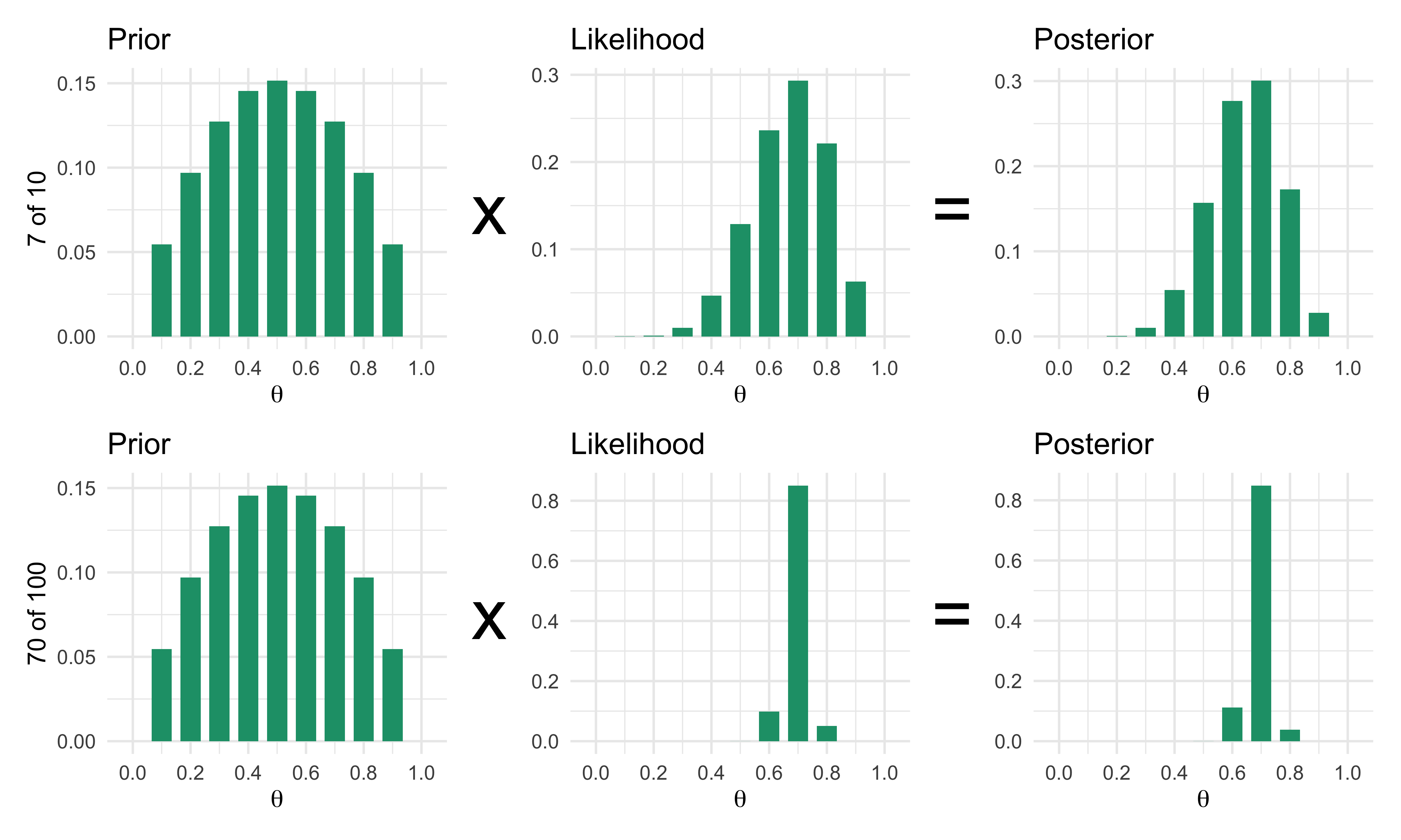
library(patchwork)theta <-seq(0, 1, by =0.1); prior <-dbeta(theta, 2, 2)grid_row <-function(h, n, lab) { g <-grid_update(theta, prior, dbinom(h, n, theta)) bar <-function(y, t, ylab =NULL) ggplot(data.frame(theta, y), aes(theta, y)) +geom_col(fill ="#1B9E77", width =0.07) +scale_x_continuous(breaks =seq(0, 1, 0.2)) +labs(x =expression(theta), y = ylab, title = t) +theme_minimal(base_size =9) sym <-function(s) ggplot() +annotate("text", 0, 0, label = s, size =9) +theme_void()bar(g$prior, "Prior", lab) +sym("x") +bar(g$likelihood, "Likelihood") +sym("=") +bar(g$posterior, "Posterior") +plot_layout(widths =c(4, 0.7, 4, 0.7, 4))}grid_row(7, 10, "7 of 10") /grid_row(70, 100, "70 of 100")
Figure 6.1: Bayes’ rule on a grid of ten-percent steps for the coin, with the Beta(2, 2) prior. Top: 7 heads in 10 tosses. Bottom: 70 heads in 100 tosses. In each row the prior times the likelihood, each rescaled to sum to one, gives the posterior. The likelihood sharpens with more data and the prior’s influence fades.
Take the grid value \(\theta = 0.7\). The prior bar is the \(\mathrm{Beta}(2,2)\) density there, \(6 \times 0.7 \times 0.3 = 1.26\), rescaled so that the eleven bars sum to one: 0.127. The likelihood bar is the probability of 7 heads in 10 tosses at \(\theta = 0.7\), 0.267, rescaled the same way: 0.293. Multiply the two bars at every grid value, then divide each product by the sum of the eleven products so that the posterior sums to one. At \(\theta = 0.7\) the result is 0.300. That is all Bayes’ rule does. In the top row the prior still counts: it pulls the posterior toward one half, and the bar at 0.6 is nearly as tall as the bar at 0.7. In the bottom row the likelihood is so narrow that any smooth prior is nearly constant across it, and the posterior is the likelihood. Make the grid finer and the bars become thin slivers along a smooth curve. With a Beta prior and a binomial likelihood those curves are Beta densities, which the rest of this section uses.
The convenient family of priors for a probability is the Beta distribution, \(\theta \sim \mathrm{Beta}(a, b)\), with density proportional to \(\theta^{a-1}(1-\theta)^{b-1}\) on \([0,1]\). Its mean is \(a/(a+b)\). \(\mathrm{Beta}(1,1)\) is the flat distribution on \([0,1]\): every value of \(\theta\) is equally believable. \(\mathrm{Beta}(2,2)\) is a gentle bell centered at one half. Larger \(a\) and \(b\) give narrower bells.
The convenience is that the likelihood of \(h\) heads and \(t\) tails, \(\theta^{h}(1-\theta)^{t}\), has the same algebraic form as the Beta density. Multiplying them as in Equation 6.1 gives
\[
\theta \sim \mathrm{Beta}(a, b), \quad h \text{ heads}, \; t \text{ tails} \quad\Longrightarrow\quad \theta \mid y \sim \mathrm{Beta}(a + h,\; b + t).
\tag{6.3}\]
A prior with this property, that the posterior belongs to the same family, is called conjugate to the likelihood. For the Beta prior and a binomial likelihood the update is addition: add the responders to \(a\) and the non-responders to \(b\). One reads \(\mathrm{Beta}(a,b)\) as “as if \(a-1\) responders and \(b-1\) non-responders had already been seen, starting from a flat prior” (with a convention that makes the rule exact, shown in the Technical note below).
Table 6.2: Beta posteriors for the coin (7 heads in 10 tosses) under the Beta(2, 2) prior of the companion lab’s coin module and a flat prior, and for the ECMO trial (11 of 11 survivors) under a flat prior.
Scenario
Posterior
Posterior mean
95% credible interval
Pr(theta > 0.8)
Coin, Beta(2, 2) prior
Beta(9, 5)
0.643
(0.386, 0.861)
0.099
Coin, flat prior
Beta(8, 4)
0.667
(0.390, 0.891)
0.161
ECMO 11/11, flat prior
Beta(12, 1)
0.923
(0.735, 0.998)
0.931
As Table 6.2 shows, with the companion lab’s Beta(2,2) prior and 7 heads and 3 tails, the posterior is Beta(9,5) with mean \(9/14 = 0.643\). With the flat prior it is Beta(8,4) with mean \(0.667\). The traditional estimate 0.70 is the value at the peak of the likelihood; the Bayesian posterior mean sits between the data and the prior’s center, and by how much depends on the prior’s strength, which we quantify shortly.
NoteTechnical note: why the update is addition
Multiply the prior density by the binomial likelihood:
which is the kernel of \(\mathrm{Beta}(a+h, b+t)\). The normalizing constant in Equation 6.1 is whatever makes the result integrate to one, namely \(B(a+h, b+t)\), so nothing needs to be integrated by hand. The statement “\(a - 1\) prior responders” holds because the flat \(\mathrm{Beta}(1,1)\) corresponds to none; some authors instead describe \(\mathrm{Beta}(a,b)\) as \(a+b\) pseudo-observations, which is the count used for effective sample size below. The two descriptions differ by the two pseudo-observations of the flat prior and are both in use.
The lab’s second scenario is a real one: Bartlett and colleagues’ 1985 trial of extracorporeal membrane oxygenation (ECMO) in newborns with respiratory failure (Bartlett et al. 1985). In the play-the-winner design, all 11 newborns assigned to ECMO survived (the single control patient did not). With a flat prior the posterior is \(\mathrm{Beta}(12, 1)\), which puts almost all its mass near survival rates close to one; Table 6.2 gives \(\Pr(\theta > 0.8) = 0.931\). This example comes back in Chapter 16, where the design rather than the analysis is the issue.
6.4 Posterior mean as a weighted average, and the prior’s effective sample size
The posterior mean of a Beta-binomial model has a form every trialist can read. Let \(n = h + t\) be the number of patients and \(\hat p = h / n\) the observed proportion. Then
\[
\mathbb{E}[\theta \mid y] = \frac{a + h}{a + b + n} = \frac{a + b}{a + b + n} \cdot \frac{a}{a+b} + \frac{n}{a + b + n} \cdot \hat p .
\tag{6.4}\]
It is a weighted average of the prior mean \(a/(a+b)\) and the sample proportion \(\hat p\), with weights proportional to \(a+b\) and \(n\). The prior acts as if it were a sample of size \(a + b\). This is the effective sample size (ESS) of a \(\mathrm{Beta}(a,b)\) prior: a flat \(\mathrm{Beta}(1,1)\) is worth two patients, a \(\mathrm{Beta}(2,2)\) four, a \(\mathrm{Beta}(30,70)\) one hundred. More refined definitions exist, which match the prior to the amount of information in the data under different criteria (Morita, Thall, and Müller 2008), and Chapter 8 treats them; for the Beta-binomial, \(a + b\) is the answer all of them roughly agree on. The prior of the BNT162b2 vaccine trial in Section 6.12, \(\mathrm{Beta}(0.700102, 1)\), has an ESS of 1.7 cases (the trial’s patients enter through the cases they produce): a prior of real shape and almost no weight.
A prior with an ESS of 10 in a trial of 200 contributes 5% of the weight; the same prior in a trial of 10 contributes half. As \(n\) grows, the data dominate and every reasonable prior gives the same posterior. This is why Bayesian analysis of a large trial with a weak prior looks like the traditional analysis, and why the debate over priors matters most in small trials, rare diseases, pediatric extrapolation and anywhere a prior of substantial ESS is deliberately used to borrow information. The FDA draft’s warning (Section IV.B.2) that conclusions can depend strongly on the prior is a statement about exactly this weight (U.S. Food and Drug Administration 2026).
Table 6.3: Weight of a Beta prior in the posterior mean for three priors and three trial sizes (45% observed response). Weight on prior is ESS/(ESS + n).
Prior
Prior ESS
Patients n
Weight on prior
Posterior mean
Sample proportion
Beta(1, 1)
2
20
0.091
0.455
0.45
Beta(1, 1)
2
100
0.020
0.451
0.45
Beta(1, 1)
2
1000
0.002
0.450
0.45
Beta(3, 7)
10
20
0.333
0.400
0.45
Beta(3, 7)
10
100
0.091
0.436
0.45
Beta(3, 7)
10
1000
0.010
0.449
0.45
Beta(30, 70)
100
20
0.833
0.325
0.45
Beta(30, 70)
100
100
0.500
0.375
0.45
Beta(30, 70)
100
1000
0.091
0.436
0.45
Table 6.3 tabulates the weights. For a prior centered at 0.30 with ESS 100 and a sample of 100 patients with a 45% response, the posterior mean is 0.375, halfway between, because the prior and the data are worth the same number of patients. With 1,000 patients the same prior moves the answer by less than 0.015.
6.5 The two-group comparison, redone
Return to the trial of Chapter 4: a control arm with a true response probability \(p_0 = 0.30\), a treatment arm with \(p_1 = 0.45\), and suppose 100 patients per arm are randomized 1:1. For the worked numbers, let the trial come out at its design values: 30 of 100 control patients respond, and 45 of 100 treatment patients respond.
The traditional analysis
The traditional analysis is the one Chapter 4 derived. The observed difference is \(\hat p_1 - \hat p_0 = 0.15\). The pooled response is \(0.375\), the standard error of the difference under the null is \(\sqrt{0.375 \times 0.625 \times (1/100 + 1/100)} = 0.0685\), so \(z = 2.19\) and the one-sided p-value is \(0.014\). Against the usual one-sided level of 0.025, this is a (modest) success. The 95% confidence interval for the difference, using the unpooled standard error 0.0676, runs from \(0.017\) to \(0.283\). Fisher’s exact test gives a one-sided p of \(0.020\).
The Bayesian analysis
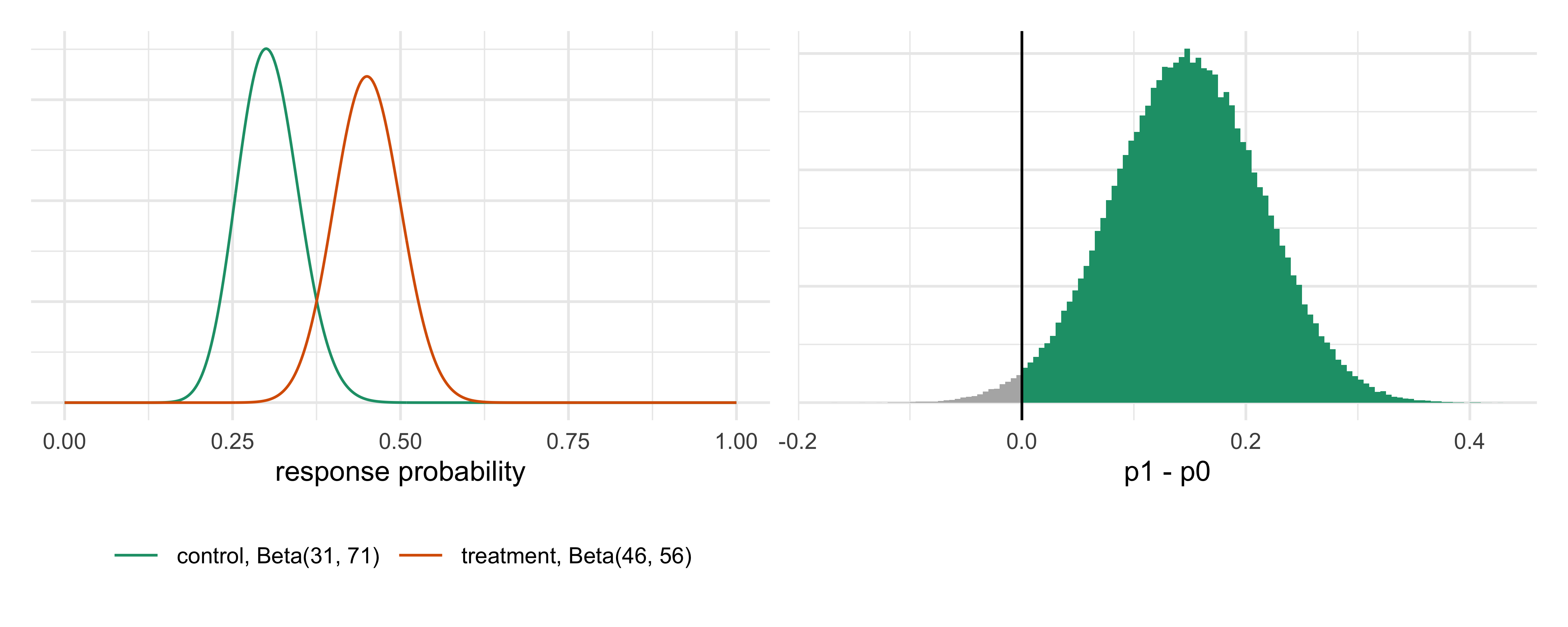
Put an independent flat \(\mathrm{Beta}(1,1)\) prior on each arm’s response rate. By Equation 6.3 the posteriors are \(p_0 \mid y \sim \mathrm{Beta}(31, 71)\) and \(p_1 \mid y \sim \mathrm{Beta}(46, 56)\), independent. The quantity of interest is a function of both parameters, the difference \(p_1 - p_0\) or the event \(p_1 > p_0\). There is no neat formula for its distribution, but there does not need to be: draw many samples from each posterior and compute the quantity of interest on the pairs. This is Monte Carlo and it is how almost every Bayesian trial quantity in this book is computed.
Table 6.4: The running trial (30/100 control and 45/100 treatment responders): traditional z test and confidence interval, and the Bayesian analysis with flat Beta(1,1) priors on each arm.
Figure 6.2: Posterior distributions after 30/100 and 45/100 responders with flat priors (left), and the posterior of the difference p1 - p0 (right). The shaded area to the right of zero is Pr(p1 > p0 | data).
The posterior probability that the treatment’s response rate exceeds the control’s is \(\Pr(p_1 > p_0 \mid y)\) = 0.9855 (Table 6.4, Figure 6.2; numerical integration; the Monte Carlo estimate with 200,000 draws is within 0.001 of it). The one-sided p-value is 0.0142, and one minus it is 0.9858. The two numbers are close because in this problem they are nearly the same calculation, as the next section shows.
The Bayesian analysis also answers questions a p-value cannot. The posterior probability that the effect exceeds 5 percentage points is 0.926; that it exceeds 10 points is 0.760. These are the quantities that enter a success criterion of the form \(\Pr(\delta > a \mid \text{data}) > c\) used in the FDA draft (Section IV.A), where \(a\) is the smallest benefit worth having and \(c\) is a pre-specified probability. Chapter 7 treats such criteria, and Chapter 14 shows how \(c\) is chosen so the design has the type I error the regulator expects. Two real trials in Section 6.12 used exactly this form: the BNT162b2 vaccine trial (success if \(\Pr(\mathrm{VE} > 30\%) > 0.986\) at the final analysis) and REMAP-CAP (efficacy if the posterior probability of benefit exceeds 99%).
A side-by-side
Table 6.5 sets the two analyses next to each other.
Table 6.5: Same trial (30/100 control and 45/100 treatment responders), analyzed the traditional way and the Bayesian way with flat priors.
\(\hat d = 0.15\), CI (0.017, 0.283), \(p = 0.014\)
mean 0.147, 95% CrI (0.015, 0.277), \(\Pr = 0.9855\)
Decision rule
reject if \(p < 0.025\)
declare success if \(\Pr(\delta > a \mid y) > c\)
What the regulator asks for
prespecified test, \(\alpha\) control
prespecified prior and \((a, c)\), calibrated operating characteristics
6.6 Why the two nearly agree
With a flat prior, the posterior of \(p_1 - p_0\) is centered, approximately, at the observed difference \(\hat d\) with standard deviation approximately equal to its standard error \(s\), and approximately normal (this is the Bernstein-von Mises phenomenon: with enough data the posterior looks like the normalized likelihood). So
The one-sided p-value for testing \(H_0: p_1 \le p_0\) is \(1 - \Phi(\hat d / s_0)\), with \(s_0\) the standard error under the null. If \(s \approx s_0\) the p-value is \(1 - \Phi(\hat d / s)\), and so \(1 - p \approx \Phi(\hat d/s)\). The two expressions are the same up to which standard error (pooled or unpooled) is used and the slight skewness of the Beta. The match is not a theorem of the model, it is a property of a flat prior and a nearly normal likelihood, and it fails when the prior is informative, when the sample is small or when the response rates are near 0 or 1. We check it numerically on many simulated trials.
Across 500 simulated trials with 100 patients per arm and true rates 0.45 and 0.30, the largest gap between \(1 - p\) and the flat-prior posterior probability (computed exactly) is 0.002, and the average gap is 0.0005.
Two cautions come with this near-equality. First, it is a numerical coincidence that has no logical force: the p-value is a statement about the data under the null, and \(\Pr(p_1 > p_0 \mid y)\) is a statement about the parameter given the data. A reader who says “\(1-p\) is the probability that the drug works” is correct in this one setting only because the prior is flat, which is itself a strong choice (it gives a prior probability of one half to the claim that treatment is better, and puts substantial mass on differences nobody believes). Second, the near-equality is what makes the Bayesian bar not lower. A trial that declares success when \(\Pr(p_1 > p_0 \mid y) > 0.975\) with a flat prior is, to a good approximation, the trial that declares success when the one-sided p-value is below 0.025. The Bayesian design’s savings, to be shown in later chapters, come from monitoring, multiple arms and prior information, not from a lower threshold at a single final analysis. Change the prior and the two diverge (Table 6.6):
Table 6.6: Posterior probability that the treatment is better than control for the running trial (45/100 against 30/100), under three priors applied to both arms.
Prior on each arm
Pr(p1 > p0 | data)
flat Beta(1,1)
0.985
Jeffreys Beta(.5,.5)
0.986
skeptical Beta(3,7), ESS 10
0.983
Applied to both arms alike, even the skeptical Beta(3,7) prior (ESS 10, mean 0.30) moves the answer only from 0.9855 to about 0.983, because 200 patients swamp 10 pseudo-patients and the prior is the same on both arms. A prior that differs between arms, or one that centers the treatment effect at zero, is a different matter and is treated in Chapter 8.
6.7 Credible intervals and confidence intervals
The 95% confidence interval for the difference is (0.017, 0.283). The 95% credible interval, the central 95% of the posterior of \(p_1 - p_0\), is (0.015, 0.277). They are numerically close, and they mean different things.
A confidence interval is a procedure. If the trial were repeated many times and the interval computed each time by the same recipe, 95% of the intervals would contain the true \(p_1 - p_0\). The probability statement is about the procedure; for the one interval in the CSR, the true value is either inside or it is not, and the “95%” does not say how likely it is that this interval covers the truth. A credible interval is a statement about the parameter: given the data and the prior, the probability that \(p_1 - p_0\) lies in the interval is 95%. There is also a choice of which 95% region, and two are common: the equal-tailed interval, leaving 2.5% in each tail, and the highest posterior density (HPD) interval, the shortest region with 95% probability. For a skewed posterior they differ; for the symmetrical one above they nearly coincide.
Many trialists read confidence intervals as if they were credible intervals, and in most large trials with weak priors they get away with it. The distinction matters in two places. One is when the prior is informative: the credible interval shifts and narrows, which is the intention, and the confidence interval cannot. The other is near boundaries, where a confidence interval built from the normal approximation may stray outside \([0,1]\) or cover poorly, while a credible interval built from the Beta posterior stays inside by construction.
Show the R code
set.seed(11); N <-20000; n <-100cover <-function(x, p) { # coverage of Wald and flat-prior credible intervals ph <- x / n; s <-sqrt(ph * (1- ph) / n) lo <-qbeta(0.025, 1+ x, 1+ n - x); hi <-qbeta(0.975, 1+ x, 1+ n - x)c(wald =mean(abs(ph - p) <1.96* s), credible =mean(lo < p & p < hi))}rows <-NULLfor (p inc(0.05, 0.30, 0.50)) { cv <-cover(rbinom(N, n, p), p) rows <-rbind(rows, data.frame(Truth =sprintf("fixed p = %.2f", p), wald = cv[["wald"]], cred = cv[["credible"]]))}p <-rbeta(N, 1, 1) # Bayesian calibration: truth drawn from the priorrows <-rbind(rows, data.frame(Truth ="p drawn from Beta(1,1)", wald =NA, cred =cover(rbinom(N, n, p), p)[["credible"]]))options(knitr.kable.NA ="")knitr::kable(rows, digits =3, col.names =c("True response rate", "Wald interval", "Flat-prior credible interval"), align ="lrr")
Table 6.7: Coverage of the Wald 95% confidence interval and the flat-prior 95% credible interval with n = 100: at fixed true response rates, and averaged over true rates drawn from the Beta(1,1) prior (20,000 simulated trials per row).
True response rate
Wald interval
Flat-prior credible interval
fixed p = 0.05
0.880
0.964
fixed p = 0.30
0.953
0.952
fixed p = 0.50
0.944
0.944
p drawn from Beta(1,1)
0.949
Table 6.7 shows the two notions of calibration. At a fixed true rate of 0.30 or 0.50, both intervals cover 94% to 95% of the time. At a rate of 0.05 the Wald interval covers only 88%, while the flat-prior credible interval covers 96.4%. Averaged over draws of \(p\) from the prior, the credible interval covers 95% by construction (94.9% in the run): if the prior is a faithful description of where true rates come from, the 95% is exact, and that is the Bayesian sense of calibration. If the prior is wrong, the coverage at a specific \(p\) can be off, which is why the FDA draft asks for operating characteristics under a range of scenarios.
6.8 The posterior predictive distribution
A trial is not only about the parameter. Decisions depend on what will happen next: how many of the next 50 patients will respond, how likely it is that the trial, if continued to its planned size, will end in success. The Bayesian answer is the posterior predictive distribution, the distribution of future data after averaging over the uncertainty about the parameter:
\[
p(\tilde y \mid y) = \int p(\tilde y \mid \theta)\, \pi(\theta \mid y)\, d\theta .
\tag{6.5}\]
For a Beta posterior \(\mathrm{Beta}(a', b')\) and \(m\) future patients, the number of future responders follows a beta-binomial distribution, which has a closed form, and its mean is \(m a' / (a' + b')\) (the posterior mean times \(m\)). The traditional analogue is a prediction interval, or more often a plug-in calculation: assume \(p = \hat p\) and compute a binomial. The plug-in ignores the uncertainty in \(\hat p\) and is therefore too narrow.
Show the R code
a <-46; b <-56; m <-50; k <-0:m # treatment-arm posterior after 45/100, next 50 patientspred <-dbetabinom(k, m, a, b) # beta-binomial pmfplug <-dbinom(k, m, 0.45)mom <-function(pm) c(mean =sum(k * pm), sd =sqrt(sum(k^2* pm) -sum(k * pm)^2))int <-function(pm) k[c(which(cumsum(pm) >=0.025)[1], which(cumsum(pm) >=0.975)[1])]draws <-rbinom(2e5, m, rbeta(2e5, a, b)) # Monte Carlo check: parameter first, then datamp <-mom(pred); mq <-mom(plug); ip <-int(pred); iq <-int(plug)knitr::kable(data.frame(Method =c("Posterior predictive (beta-binomial)", "Plug-in binomial, p = 0.45", "Monte Carlo check"),Mean =c(mp[[1]], mq[[1]], mean(draws)), SD =c(mp[[2]], mq[[2]], sd(draws)),Lower =c(ip[1], iq[1], unname(quantile(draws, 0.025))), Upper =c(ip[2], iq[2], unname(quantile(draws, 0.975)))),digits =c(0, 2, 2, 0, 0), col.names =c("Method", "Mean", "SD", "95% interval, lower", "95% interval, upper"), align ="lrrrr")
Table 6.8: Number of responders among the next 50 patients, given 45/100 so far and a flat prior: posterior predictive distribution against the plug-in binomial with p = 0.45.
Method
Mean
SD
95% interval, lower
95% interval, upper
Posterior predictive (beta-binomial)
22.55
4.27
14
31
Plug-in binomial, p = 0.45
22.50
3.52
16
29
Monte Carlo check
22.56
4.28
14
31
In Table 6.8 the predictive mean is 22.5 responders out of 50 and its standard deviation is 4.27, against 3.52 for the plug-in binomial. The extra spread is the contribution of not knowing \(p\): a prediction made as if \(\hat p = 0.45\) were the truth would be overconfident by about 20 percent. The 95% predictive interval for responders among the next 50 is 14 to 31, which the Monte Carlo agrees with.
The same two-stage logic, “draw the parameter from its posterior, then draw the future data from the model,” gives the predictive probability that a trial in progress will succeed at its final analysis. Chapter 15 builds on exactly Equation 6.5 to define predictive probability, futility rules and Goldilocks-type sample-size choices.
6.9 Normal-normal on the log hazard ratio
Many pivotal trials, in oncology, cardiovascular disease and neurology, do not have a binary endpoint but a time to event, and the treatment effect is a hazard ratio (HR). The Beta-binomial model does not apply. The normal-normal model, which does, rests on a standard approximation.
For 1:1 randomization with \(d\) total events, the log hazard ratio estimate has standard error \(\approx 2/\sqrt{d}\). (Each arm contributes about \(d/2\) events and the variance of a log hazard ratio is about \(1/d_1 + 1/d_0 = 4/d\).) With \(\theta = -\log \mathrm{HR}\), so that a positive \(\theta\) means benefit, the data are summarized by
This is the likelihood, an approximate one: the Cox partial likelihood in large samples is close to a normal in \(\theta\), and the approximation is the standard route taken by Bayesian design in survival studies. In the traditional trial the logrank test is, to a good approximation, the z test \(z = \hat\theta \sqrt{d} / 2\), and the one-sided p-value is \(1 - \Phi(z)\). The number of events, not patients, is the sample size, in both frameworks; this chapter uses the same events-as-information language that Chapter 9 and Chapter 11 use.
Take a trial that observes \(d = 200\) events and \(\widehat{\mathrm{HR}} = 0.74\), so \(\hat\theta = -\log 0.74 = 0.30\) with standard error \(2/\sqrt{200} = 0.141\). Then \(z = 2.12\) and the one-sided p-value is \(0.017\), a success at the 0.025 level.
For the prior take a normal distribution, \(\theta \sim N(m_0, \tau^2)\). A normal prior and a normal likelihood give a normal posterior (normal-normal conjugacy), with precision (the reciprocal of the variance) equal to the sum of the precisions:
This is the same weighted average of Equation 6.4, now with weights given by precision. The data have precision \(d/4\), so each event carries a quarter of a unit of precision, and a prior of variance \(\tau^2\) carries \(1/\tau^2\). The effective sample size of the prior, in events, is therefore \(4/\tau^2\): a prior \(N(0, 0.2^2)\) is worth 100 events, and \(N(0, 0.35^2)\) is worth about 33.
Table 6.9: Posterior for theta = -log HR with 200 events and an observed hazard ratio of 0.74, under a flat, a skeptical and a strong skeptical normal prior. Pr(HR < 0.9) is the posterior probability that the hazard ratio is below the margin 0.9.
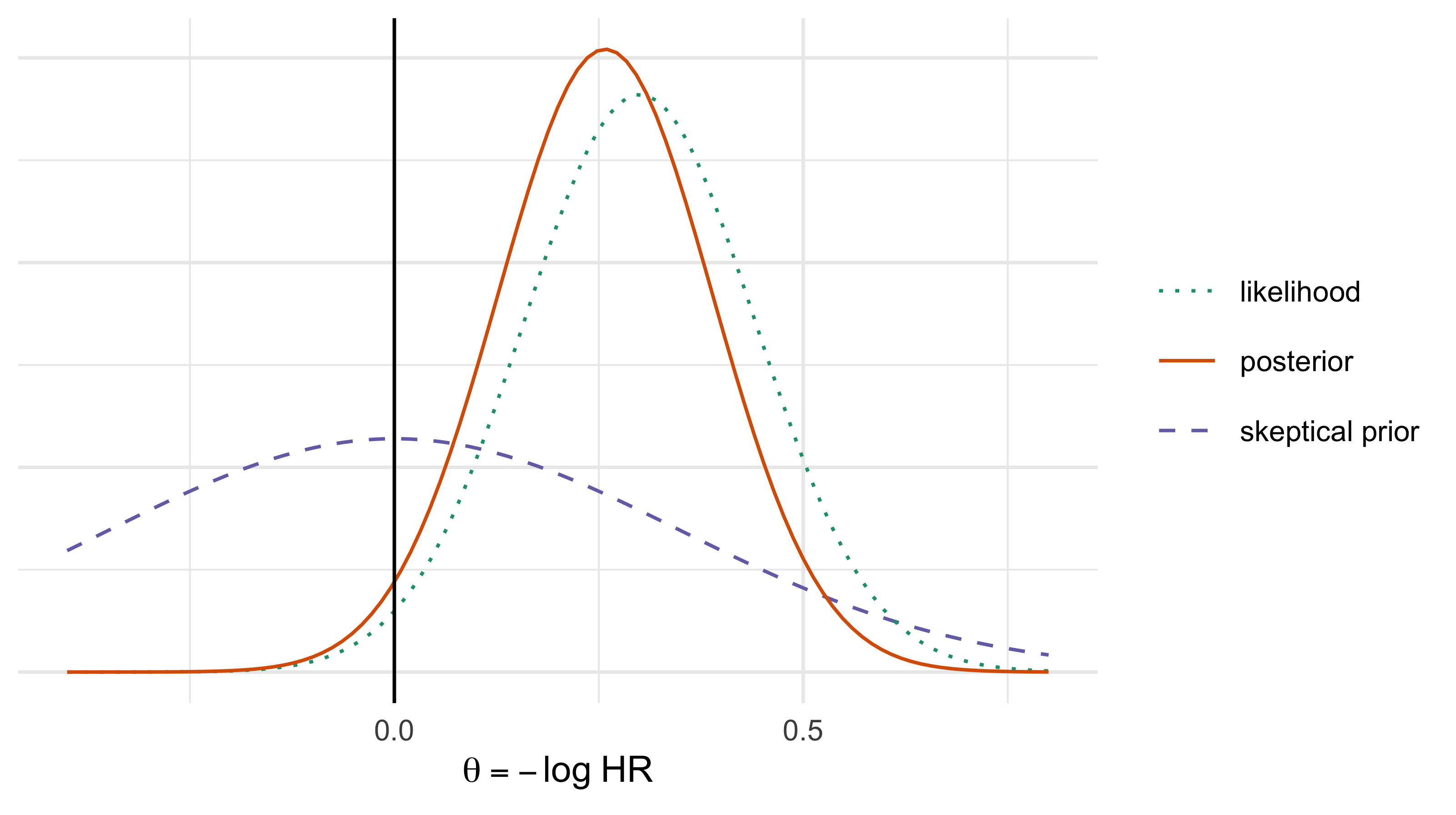
Figure 6.3: Prior, likelihood and posterior for theta = -log HR with 200 events and an observed hazard ratio of 0.74. The skeptical prior N(0, 0.35^2) pulls the posterior toward no effect.
Table 6.9 gives the three posteriors. With a flat prior (Figure 6.3 shows the skeptical case), the posterior is \(N(0.300, 0.141^2)\) and \(\Pr(\theta > 0 \mid \hat\theta) = 0.983\). That is \(1 - p\) again, to within the third decimal place (\(1 - 0.017 = 0.983\)), and now exactly: in the normal-normal model with a flat prior, \(\Pr(\theta > 0 \mid \hat\theta) = \Phi(\hat\theta/\text{se})\) is identically one minus the one-sided p-value, so the agreement of the previous section is an identity here. With a skeptical prior of ESS 33 events, the posterior mean is 0.258 (HR 0.77), \(\Pr(\theta > 0) = 0.975\) and the 95% credible interval for the hazard ratio is about 0.60 to 1.00. With the stronger skeptical prior (ESS 100) the posterior mean drops to 0.200 (HR 0.82) and the credibility of any benefit falls to 0.958. The same data under three priors give 0.983, 0.975 and 0.958: at a threshold of 0.975 the first passes, the second passes only in the fourth decimal, and the third fails. This is why the prior must be specified before the data, and why Chapter 8 is about how to choose one that a regulator will accept.
NoteTechnical note: normal-normal in one line
Complete the square. The product of \(\exp\{-(\theta - m_0)^2 / 2\tau^2\}\) and \(\exp\{-(\hat\theta - \theta)^2 d/8\}\) is proportional to \(\exp\{-\tfrac12(1/\tau^2 + d/4)\,\theta^2 + (m_0/\tau^2 + \hat\theta\, d/4)\,\theta\}\), which is the kernel of a normal with precision \(1/\tau^2 + d/4\) and mean the ratio of the linear to the quadratic coefficient. The approximation in Equation 6.6 is a modeling choice, not an exact result: it treats \(\hat\theta\) as sufficient for the log hazard ratio, which holds only approximately for a Cox model, and it ignores the discreteness of event times. For design purposes it is the usual choice; the final analysis in a Bayesian trial that wants the exact partial or full likelihood can use a piecewise exponential model.
6.10 Sequential updating: the posterior today is the prior tomorrow
A trial accrues over months or years. Suppose data arrive in batches, \(y_1\) and then \(y_2\). Bayes’ rule can be applied twice: first to the prior and \(y_1\), giving \(\pi(\theta \mid y_1)\), then to \(\pi(\theta \mid y_1)\) taken as the prior and \(y_2\):
provided \(y_1\) and \(y_2\) are conditionally independent given \(\theta\) (which is what exchangeability delivers). The last expression is the posterior obtained from all data at once with the original prior. Updating in batches, one patient at a time or all at once, gives the same posterior: the posterior today is the prior tomorrow, and the path by which the data arrived does not matter.
Show the R code
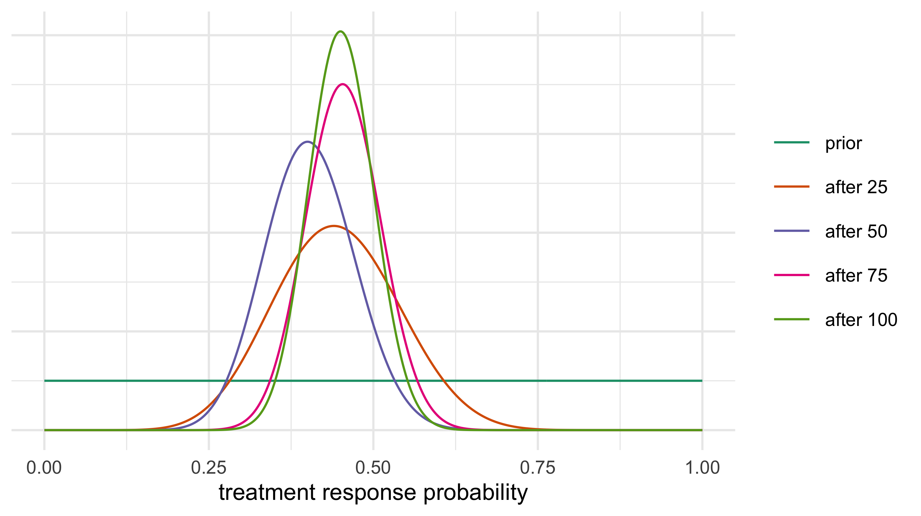
r <-c(11, 9, 14, 11); m <-rep(25, 4) # responders and patients per batch, total 45/100a <-1; b <-1; grid <-seq(0, 1, length.out =500)curves <-data.frame(x = grid, y =dbeta(grid, a, b), stage ="prior")for (k in1:4) { a <- a + r[k]; b <- b + m[k] - r[k] curves <-rbind(curves, data.frame(x = grid, y =dbeta(grid, a, b), stage =paste("after", 25* k)))}stopifnot(a ==1+sum(r), b ==1+100-sum(r)) # same as the one-step update with all 100curves$stage <-factor(curves$stage, unique(curves$stage))ggplot(curves, aes(x, y, colour = stage)) +geom_line() +scale_colour_brewer(palette ="Dark2") +labs(x ="treatment response probability", y =NULL, colour =NULL) +theme_minimal(base_size =9) +theme(axis.text.y =element_blank())
Figure 6.4: Posterior of the treatment response rate as 100 patients accrue in four batches of 25, starting from a flat prior. The last curve is also the posterior from all 100 patients at once.
The assertion at the end of the chunk (and the last curve of Figure 6.4) is the whole point: the four-step posterior is \(\mathrm{Beta}(46, 56)\), the same as the one-step posterior of Section 6.5. For conjugate models the batch-wise update is just a running total of responders and non-responders, which is why Bayesian interim analyses are cheap computationally: the interim posterior is a handful of arithmetic operations, and a Data Monitoring Committee can be given it at any time.
Looking does not change the posterior
The traditional trialist’s reaction to the last paragraph is that something has been skipped. In a group sequential design (the subject of Chapter 11) every look at the data costs something: the nominal level at each look is reduced, because testing five times at 0.025 does not preserve a type I error of 0.025. Yet the Bayesian posterior at any interim analysis is computed with exactly the same formula as the posterior at the end, and it does not know how many looks preceded it. How can both statements be true?
They are answers to different questions. The likelihood principle says that, given the data, the evidence about \(\theta\) in an experiment depends on the data only through the likelihood function, and not on the stopping rule or on what other results might have been observed but were not (Berger and Wolpert 1988). The posterior depends on the data through the likelihood only, so it is unchanged by the decision to look, or by the decision to stop because the posterior crossed a threshold. A p-value, by contrast, is a statement about all the data sets the procedure could have produced, and which data sets those are depends on the stopping rule: “stop at the first of five looks where \(z > 1.96\)” is a different procedure from “analyze once at the end,” and has a different sampling distribution. The type I error rate is a property of the procedure over repeated trials under the null, so it is changed by looking. The posterior probability, a statement about this trial’s parameter given this trial’s data, is not.
We can see both statements in one simulation of the trial of this chapter. Five looks at 50 patients per arm (cumulative n = 50, 100, 150, 200, 250 per arm).
Show the R code
res <-sim_sequential_looks(n_trials =4000, n_look =50, n_looks =5, seed =11)knitr::kable(data.frame(Setting =c(rep("Null true (p1 = p0 = 0.30), one-sided z > 1.96", 2), rep("Truth drawn from flat priors, stop at first look with Pr(p1 > p0 | y) > 0.975", 3)),Quantity =c("Rejection rate, one look at the end", "Rejection rate, any of 5 looks", "Trials that stopped (of 4000)","Mean posterior probability at stopping", "Fraction of stopped trials where p1 > p0 truly"),Value =c(sprintf("%.3f", res$final_only), sprintf("%.3f", res$any_look), sprintf("%d", res$n_stopped), sprintf("%.4f", res$mean_post_at_stop), sprintf("%.4f", res$frac_truly_better))),align ="llr")
Table 6.10: Simulation of five looks at 50 patients per arm (4000 trials): frequentist rejection rates under the null, and the behavior of a Bayesian stopping rule when the truth is drawn from the prior used in the analysis.
Setting
Quantity
Value
Null true (p1 = p0 = 0.30), one-sided z > 1.96
Rejection rate, one look at the end
0.024
Null true (p1 = p0 = 0.30), one-sided z > 1.96
Rejection rate, any of 5 looks
0.069
Truth drawn from flat priors, stop at first look with Pr(p1 > p0 | y) > 0.975
Trials that stopped (of 4000)
1776
Truth drawn from flat priors, stop at first look with Pr(p1 > p0 | y) > 0.975
Mean posterior probability at stopping
0.9969
Truth drawn from flat priors, stop at first look with Pr(p1 > p0 | y) > 0.975
Fraction of stopped trials where p1 > p0 truly
0.9955
Table 6.10 has two blocks. The first is the frequentist finding: with the null true and five looks at the nominal one-sided 0.025 level, the chance of declaring success at some look is 0.069, not 0.025 (the final-look-only rate in this simulation is 0.024). That is the reason group sequential designs adjust the thresholds, and the reason regulators insist that the monitoring plan be prespecified (ICH E9 Section 4.5 on interim analysis). The second is the Bayesian finding. When the true response rates are drawn from the prior that the analysis assumed, the trials that stop at a looked-at threshold of 0.975 have, on average, a posterior probability of 0.9969 at the moment they stop, and the fraction of those trials in which the treatment is truly better is 0.9955. The posterior is right on average among the trials that stopped, despite the five opportunities to stop.
Two cautions keep this from being an overstatement.
Stopping-rule invariance follows from the likelihood factorization: for an ignorable stopping mechanism and a fixed analysis prior, the stopping factor cancels. Calibration across trials additionally depends on the assumed prior and sampling model. The calibration in the second block was produced by drawing truth from the same prior the analysis used. If the true effects are not drawn from that prior, then the posterior at the moment of stopping is not calibrated to anything in the real world, and the frequentist inflation reappears as an operating characteristic: the fraction of null drug trials that stop for success is what the regulator cares about, and it is a property of the design and the threshold, not of the posterior at a single look. For this reason one of the routes the FDA draft describes, and this book’s default for confirmatory adaptive designs without borrowing, is to calibrate Bayesian success criteria by simulation to the type I error probability, and E20 Section 5.3 describes the same operating characteristics (U.S. Food and Drug Administration 2026; International Council for Harmonisation 2025). Chapter 14 shows how.
Having a valid posterior at every look does not make every look free. Looks cost in the currency of operating characteristics: a threshold chosen to be right at a single look must be raised, or the number of looks limited, if the design is to hold the type I error at 0.025 across the monitoring plan. Chapter 11 quantifies the price. What the likelihood principle removes is the conceptual objection that Bayesian inference “does not know about” the looks; what it does not remove is the regulator’s requirement, in practice, that it be shown that it does not matter.
A Bayesian primary analysis needs, at minimum, the following statements in the protocol or the statistical analysis plan. They follow from the definitions of this chapter and from the FDA draft’s emphasis on prespecification.
The model: the sampling distribution of the endpoint given the parameter (for example, binomial with response probability \(p_j\) in arm \(j\); or \(\hat\theta \sim N(\theta, 4/d)\) for \(\theta = -\log \mathrm{HR}\)).
The prior for every parameter, with its form and values (for example, \(p_j \sim \mathrm{Beta}(1, 1)\) for both arms), its effective sample size, and the reasoning behind it. The prior is specified before the data are unblinded.
The quantity on which the decision is made, with its threshold (for example, \(\Pr(p_1 - p_0 > 0 \mid \text{data}) > 0.975\), or the Pfizer-BioNTech rule \(\Pr(\mathrm{VE} > 30\%) > 0.986\) at the final analysis and \(> 0.995\) at interims), so that the success criterion is explicit.
The computation: whether the posterior is analytic or by Monte Carlo (and with how many draws, and with what seed and software), so that the result can be reproduced.
The operating characteristics: type I error and power by simulation under the stated scenarios, referred to in the simulation report (Chapter 14).
A statement of how the traditional analysis (estimate, confidence interval, p-value) will be reported alongside, if the sponsor wants the Bayesian analysis to be read against it.
6.12 In practice: two trials that stated their success rule as a posterior probability
Pfizer-BioNTech BNT162b2, phase 3 (C4591001)
The phase 2/3 trial of the BNT162b2 mRNA vaccine is the cleanest large example of this chapter’s machinery. Its statistical analysis plan [Pfizer Inc. (2022), Section 7.1 and Appendix 2; the document at the cited ClinicalTrials.gov address is version 10, dated 7 October 2022, and is not an archived 2020 version] used a beta-binomial model, conditional on the total number of first COVID-19 cases \(s\), of whom \(s_1\) occur in the vaccine arm. With equal allocation and equal follow-up, a case falls in the vaccine arm with probability \(p = (1 - \mathrm{VE})/(2 - \mathrm{VE})\), where VE is the vaccine efficacy, one minus the ratio of incidence rates. Then \(s_1 \mid s \sim \mathrm{Binomial}(s, p)\), and the prior is \(p \sim \mathrm{Beta}(0.700102, 1)\). Its mean is \(0.4118\), the value of \(p\) at VE \(= 30\%\), so the prior is centered on the efficacy margin, and the plan calls it minimally informative and says it can be considered pessimistic. Its 95% interval for \(p\) is \((0.005, 0.964)\), which is \((-26.2, 0.995)\) for VE written as a fraction, about \(-2{,}620\%\) to \(99.5\%\): the lower limit corresponds to an incidence rate ratio of 27.2, a vaccine arm with 27 times the cases of the placebo arm, and the interval is nearly the whole admissible range, as a weak prior should be. The ESS of Section 6.4 is \(a + b = 1.7\) cases.
The success criterion was a posterior probability, as in the form \(\Pr(\delta > a \mid \text{data}) > c\) above: efficacy is declared if \(\Pr(\mathrm{VE} > 30\% \mid \text{data}) > 0.986\) at the final analysis, and if it exceeds \(0.995\) at an interim analysis. The plan states that the two thresholds were calibrated so that the overall one-sided type I error is \(2.5\%\), which is the regulator’s language from Section 6.11 applied to a Bayesian rule. The final analysis was planned at 164 cases, with interim looks at 62, 92 and 120 cases (a look at 32 cases was in the plan and not performed, and the thresholds were unchanged). The trial reported \(8\) cases with onset at least 7 days after the second dose in the vaccine group against \(162\) in the placebo group (Polack et al. 2020), so \(s = 170\) and \(s_1 = 8\). The posterior is \(\mathrm{Beta}(0.700102 + 8,\; 1 + 162)\), and everything follows from base R.
Show the R code
a0 <-0.700102; b0 <-1# prior on p = (1 - VE) / (2 - VE)ve <-function(p) (1-2* p) / (1- p) # VE as a function of ppost <-beta_post(8, 170, a0, b0) # 8 vaccine cases out of 170 (8 vs 162)p30 <-0.7/1.7# p at VE = 30%pr_fail <-pbeta(p30, post$a, post$b, lower.tail =FALSE) # Pr(VE < 30% | data)q <-100*ve(qbeta(c(0.975, 0.5, 0.025), post$a, post$b)) # VE is decreasing in pknitr::kable(data.frame(Quantity =c("Prior mean of p", "Prior effective sample size", "Prior 95% interval for VE (as a fraction)", "Posterior of p","Pr(VE < 30% | data)", "Posterior median VE", "95% credible interval for VE", "Plug-in VE, 1 - IRR"),Value =c(sprintf("%.4f", a0 / (a0 + b0)), sprintf("%.1f", ess_beta(a0, b0)), sprintf("(%.1f, %.3f)", ve(qbeta(0.975, a0, b0)), ve(qbeta(0.025, a0, b0))),sprintf("Beta(%.6f, %g)", post$a, post$b), sprintf("%.1e", pr_fail), sprintf("%.1f%%", q[2]), sprintf("(%.1f%%, %.1f%%)", q[1], q[3]), sprintf("%.1f%%", 100*ve(8/170)))),align ="lr")
Table 6.11: Reproduction of the BNT162b2 analysis: prior and posterior for p = (1 - VE)/(2 - VE) with 8 vaccine cases among 170, and the implied vaccine efficacy (VE).
Quantity
Value
Prior mean of p
0.4118
Prior effective sample size
1.7
Prior 95% interval for VE (as a fraction)
(-26.2, 0.995)
Posterior of p
Beta(8.700102, 163)
Pr(VE < 30% | data)
2.0e-28
Posterior median VE
94.9%
95% credible interval for VE
(90.4%, 97.6%)
Plug-in VE, 1 - IRR
95.1%
Table 6.11 gives the prior and the posterior. The posterior probability that VE exceeds 30% is \(1 - 2 \times 10^{-28}\), which clears \(0.986\). The 95% credible interval for VE, the equal-tailed interval of the posterior of \(p\) transformed through the monotone map \(p \mapsto \mathrm{VE}\), is about \((90.4\%, 97.6\%)\), and the point estimate is \(95.1\%\) (plug-in) or \(94.9\%\) (posterior median). The paper reports \(95.0\%\) with 95% credible interval \(90.3\) to \(97.6\)(Polack et al. 2020), so the chapter’s calculation reproduces it to within a tenth of a point on the lower limit; we did not model the small difference in surveillance time between the arms, which is the likely source. Two lessons for the chapter’s method. First, a Bayesian rule can be stated entirely as a threshold on a posterior probability and still be calibrated to a type I error, so the regulator reads it as it would read a boundary on a test statistic. Second, with \(\mathrm{ESS} = 1.7\) and 170 cases the prior is irrelevant to the conclusion, and a different prior, such as a flat \(\mathrm{Beta}(1,1)\), would shift the interval by well under a point. The prior was chosen to be defensible, not to carry the result. The FDA authorized the vaccine for individuals 16 years and older on 11 December 2020 (U.S. Food and Drug Administration 2021), and approved the biologics license on 23 August 2021. The public record used here is the statistical analysis plan, the trial report and the authorization notice; the agency’s own assessment of the Bayesian criterion is not summarized. Chapter 8 returns to pessimistic priors on the margin, and Chapter 15 to the futility rule in the same plan.
REMAP-CAP: posterior probabilities of benefit as the reported result
REMAP-CAP is a platform trial (Chapter 20) whose primary analysis is a Bayesian cumulative logistic model for organ support-free days to day 21. The report on interleukin-6 receptor antagonists (REMAP-CAP Investigators et al. 2021) states the rules as posterior probabilities, fixed in advance: efficacy if the posterior probability that the odds ratio exceeds 1 is above 99%, futility if the posterior probability that the odds ratio exceeds 1.2 is below 5%, and equivalence if the probability that the odds ratio between two non-control interventions lies between 0.83 and 1.2 exceeds 90%. Priors on the individual treatment effects were neutral. At an interim analysis in 2020, tocilizumab crossed the efficacy threshold with posterior probability \(99.75\%\). The chronology and final estimates are in Chapter 20. The lesson is the one of Section 6.5 at scale: the result is a posterior probability checked against a prespecified threshold, the stopping time is determined by when it crosses and not by a fixed sample size, and the reader is told, in the same units, how far above the threshold the evidence was. The posterior being valid at each look (Section 6.10) is what lets the platform report while it continues.
6.13 Summary: what changed, what stayed
Starting from the traditional two-group comparison, the Bayesian version changed three things and left a fourth alone.
The unknown becomes a distribution. The treatment effect is described by a prior, updated by data into a posterior, and statements are probabilities about the effect.
The inputs gain a prior. The prior has to be chosen, prespecified and defended; it is worth a stated number of patients (its effective sample size).
The outputs change meaning. The credible interval is a probability statement about the parameter, \(\Pr(p_1 > p_0 \mid y)\) is a probability that the treatment is better, and posterior predictive distributions say what future patients will do.
The data’s role does not change. The likelihood is the same one the traditional trial uses, and with a flat prior and a large trial the numbers agree: \(\Pr(p_1 > p_0 \mid y) = 0.9855\) against \(1 - p = 0.9858\) here, and exactly \(1 - p\) in the normal-normal model.
The regulator’s position, stated in ICH E9 and reaffirmed in the FDA draft and E20, is that the Bayesian approach is acceptable when the reasons for its use are clear and the conclusions are robust. Robust here is a technical word: the conclusion should survive a reasonable change of prior, and the design should have operating characteristics, demonstrated by simulation, that a regulator can read in the language of error rates. Chapter 7 takes up the weighing of evidence, Chapter 8 the choice of priors, and Chapter 11 and Chapter 15 the use of the posterior and the predictive distribution in monitoring.
TipTry it in the lab
Open module 01 of the companion lab, Prior and posterior. Before pressing “Toss 10,” predict where the posterior will peak after 7 heads and 3 tails starting from a flat prior and from the Beta(2,2) prior (the modes are 7/10 = 0.70 and 8/12 = 0.667; the means are 8/12 = 0.667 and 9/14 = 0.643, as in Section 6.3). Then load the “Newborn trial (real)” example and note how a single arm of 11 successes concentrates the posterior near 1 even from a flat start.
Key points
Bayes’ rule reverses a conditional probability: posterior is proportional to prior times likelihood. The diagnostic-test example, with a 27% positive predictive value from a 90% sensitive, 95% specific test at 2% prevalence, is the same logic as a trial posterior.
Exchangeability, the judgment that the order of patients does not matter, replaces independence; de Finetti’s theorem turns it into a likelihood and a prior. It can fail. Randomization makes treatment assignment independent of prognosis; the response model separately assumes exchangeability within each arm or stratum.
The Beta prior is conjugate to the binomial: the update adds responders and non-responders. The posterior mean is a weighted average of prior mean and sample proportion, and the prior’s effective sample size is \(a + b\).
With flat priors, \(\Pr(p_1 > p_0 \mid y) = 0.9855\) matches \(1 - p = 0.9858\) for the trial of 45/100 versus 30/100, and across simulated trials the two differ by at most 0.002. In the normal-normal model on \(\theta = -\log \mathrm{HR}\) the match is exact. A Bayesian threshold of 0.975 with a flat prior is not a lower bar than a one-sided 0.025.
A confidence interval describes a procedure and a credible interval describes a parameter. Predictive distributions, which add the uncertainty about the parameter to the sampling variability, are wider than plug-in predictions and are the basis of predictive probability.
The posterior at an interim look is the same function of the data whatever the stopping rule, but the type I error of a stopping rule is not; the first is a statement about this trial, the second about repeated trials. Regulators judge a Bayesian design by the second, which is why the FDA draft recommends prior prespecification and evaluated operating characteristics, with calibration to type I error as one of its three routes and this book’s default.
NoteDiscussion questions
A sponsor states that “the p-value of 0.014 means there is a 98.6% probability that the drug works.” Under what assumptions is the number right, what is the claim’s problem, and how would you rephrase it for the clinical study report?
A Beta(30, 70) prior is proposed for the control arm from a historical trial of 100 patients. What is its effective sample size, how much of the posterior mean would it contribute in a current trial with 50 control patients, and what would you ask the sponsor to show about the exchangeability of the historical and current patients?
A Data Monitoring Committee is shown, after 150 events, a posterior probability of benefit of 0.96 under a skeptical prior and 0.99 under a flat prior. What would you need to know to decide which number to rely on, and what does the protocol have to have said beforehand?
A colleague says Bayesian monitoring is free because the posterior is unaffected by looking. Using the simulation of the previous section, explain what is true in that sentence and what is not.
ICH E9 permits Bayesian approaches when “the reasons for their use are clear and when the resulting conclusions are sufficiently robust.” Draft two sentences for a protocol that meet that expectation for the normal-normal analysis of Section 6.9.
Bartlett, Robert H., Daniel W. Roloff, Richard G. Cornell, Alvin F. Andrews, Patricia W. Dillon, and Joseph B. Zwischenberger. 1985. “Extracorporeal Circulation in Neonatal Respiratory Failure: A Prospective Randomized Study.”Pediatrics 76 (4): 479–87.
Berger, James O. 1985. Statistical Decision Theory and Bayesian Analysis. 2nd ed. New York: Springer-Verlag.
Berger, James O., and Robert L. Wolpert. 1988. The Likelihood Principle. 2nd ed. Vol. 6. IMS Lecture Notes, Monograph Series. Hayward, CA: Institute of Mathematical Statistics.
de Finetti, Bruno. 1937. “Foresight: Its Logical Laws, Its Subjective Sources.” In Studies in Subjective Probability, edited by Henry E. Kyburg and Howard E. Smokler, 93–158. New York: Wiley.
Edwards, Ward, Harold Lindman, and Leonard J. Savage. 1963. “Bayesian Statistical Inference for Psychological Research.”Psychological Review 70 (3): 193–242.
Gelman, Andrew, John B. Carlin, Hal S. Stern, David B. Dunson, Aki Vehtari, and Donald B. Rubin. 2013. Bayesian Data Analysis. 3rd ed. Chapman; Hall/CRC. https://doi.org/10.1201/b16018.
Polack, Fernando P., Stephen J. Thomas, Nicholas Kitchin, et al. 2020. “Safety and Efficacy of the BNT162b2mRNACovid-19 Vaccine.”New England Journal of Medicine. https://doi.org/10.1056/NEJMoa2034577.
REMAP-CAP Investigators, Anthony C. Gordon, Paul R. Mouncey, Farah Al-Beidh, Kathryn M. Rowan, Alistair D. Nichol, et al. 2021. “Interleukin-6 Receptor Antagonists in Critically Ill Patients with Covid-19.”New England Journal of Medicine 384 (16): 1491–1502. https://doi.org/10.1056/NEJMoa2100433.
Savage, Leonard J. 1954. The Foundations of Statistics. Wiley.
U.S. Food and Drug Administration. 2021. “Emergency Use Authorization Letter, Pfizer-BioNTechCOVID-19 Vaccine (Reissued 10 May 2021; Original EUA 11 December 2020).”https://www.fda.gov/media/144412/download.