A sponsor planning a trial of a new drug in a rare disease already knows something about the control arm. Earlier trials enrolled similar patients, a registry holds their outcomes, and a pediatric program can lean on what is known in adults. Using that knowledge looks like plain common sense, and there is a cost argument too: every patient who does not have to be randomized to control is a patient who can be treated, or a trial that can finish sooner. This chapter is about how to use such information, how regulators judge it, and what it costs when the borrowed information turns out to be wrong.
Of the four mechanisms by which Bayesian designs save patients (monitoring, multiple arms, shrinkage, and prior information), borrowing is the one with the sharpest trade. Done well, it recovers precision that a small trial cannot supply. Done badly, it can introduce substantial bias into a small current trial, whose data may be insufficient to reveal the mismatch, and it does so under the sponsor’s own prior. The central message of the chapter is that borrowing is not free, that the price is measurable by simulation, and that the regulator will ask to see that price before agreeing to the design.
ImportantRegulatory anchor
FDA draft guidance, Use of Bayesian Methodology in Clinical Trials of Drug and Biological Products (January 2026, draft)(U.S. Food and Drug Administration 2026). Informative priors “will generally need a greater amount of justification”. Discusses static versus dynamic discounting, effective sample size (ESS), prior-data conflict and sensitivity analyses. Recommends against measuring the amount of borrowing by type I error inflation. Case examples include REBYOTA, pediatric extrapolation, platform-trial controls and basket trials. Details in Chapter 3.
ICH E10, Choice of Control Group (Step 4, July 2000)(International Council for Harmonisation 2000). Names the externally (historically) controlled trial as one of the five types of control and states its main weakness, the inability to control bias.
FDA draft guidance, Considerations for the Design and Conduct of Externally Controlled Trials (February 2023, draft)(U.S. Food and Drug Administration 2023a). Recommendations for building external control arms from real-world data, with emphasis on pre-specification and comparability.
FDA, Considerations for the Use of Real-World Data and Real-World Evidence to Support Regulatory Decision-Making for Drug and Biological Products (final guidance, August 2023)(U.S. Food and Drug Administration 2023b). FDA’s current thinking on how real-world data and evidence support new indications and postapproval studies. It recommends and does not require, and for external control arms it refers to the externally controlled trials draft above.
FDA, Rare Diseases: Considerations for the Development of Drugs and Biological Products (final guidance, December 2023)(U.S. Food and Drug Administration 2023c). Finalizes the draft “Rare Diseases: Common Issues in Drug Development” of February 1, 2019. It says that external control designs are usually reserved for specific circumstances, such as a well-understood and characterized natural history, high and predictable mortality or progressive and predictable morbidity, or a drug effect that is large and self-evident, that each such design warrants a case-by-case assessment, and that early discussion with the review division is recommended. It also says that sponsors may be able to use Bayesian methods to maximize the use of information from early-phase or natural history studies, and that Bayesian methods may inform pediatric investigations through incorporation of adult data.
ICH E11A, Pediatric Extrapolation (Step 4, August 2024)(International Council for Harmonisation 2024). A framework for deciding how much pediatric efficacy can be inferred from adult or other source data, and a place for Bayesian methods in the quantitative part.
FDA, Guidance for the Use of Bayesian Statistics in Medical Device Clinical Trials (final, February 2010)(U.S. Food and Drug Administration 2010). The device guidance that has allowed borrowing from prior studies for more than fifteen years, with simulated operating characteristics.
19.1 What the traditional design does with prior data
A traditional trial uses prior data heavily, but only before the trial starts. Phase 2 results and earlier studies of the control treatment set the design alternative (the effect size the trial is powered to detect), the assumed control response rate or event rate, the variance, the dropout rate, and therefore the sample size. In the notation of Chapter 9, the sample size is a function of \(\theta\) and of nuisance parameters, and all of them come from earlier data. A sponsor who assumed a 30% control response rate because three earlier trials averaged 30% has used those trials fully.
Then the data are set aside. In a conventional standalone randomized-trial analysis, the analysis of the new trial uses only the new trial. The earlier studies appear in the introduction of the protocol and in the clinical overview, and nowhere in the p-value or the confidence interval. This is the usual convention, and it has a reason. The frequentist guarantee, a one-sided type I error of 0.025 at every parameter value in the null hypothesis, is a statement about repeated use of the same procedure on the same kind of data. If last year’s data entered this year’s test statistic, the guarantee would depend on how last year’s data happen to relate to this year’s patients, and nothing in the protocol controls that. Frequentist methods can incorporate historical information under explicit assumptions (the margin synthesis later in this chapter is one, and FDA’s 2016 noninferiority guidance describes a frequentist synthesis method that combines the historical and current estimates and their uncertainties (U.S. Food and Drug Administration 2016)), but the guarantee then holds only under those assumptions.
The rule has a cost that is easy to see in a small trial. If the control arm must be as large as the treatment arm, half of a scarce population is randomized to a comparator whose behavior is, to a good approximation, already known. In a pediatric rare-disease program the number of eligible children may not support a trial of conventional size at all. The traditional design answers this with a smaller trial and a looser level of evidence, a larger effect size in the alternative, or a single-arm design. The single-arm design is where the question of external information becomes unavoidable.
19.2 External and historical controls: the traditional objections
In a single-arm trial all patients receive the new treatment, and the effect is judged by comparing the observed outcome with what is expected without it. The expectation comes from somewhere: a published control arm, a registry, a set of earlier trials, a cohort of patients treated in routine care. ICH E10 calls this the externally controlled trial, including the historical control, and lists it among the five kinds of control group (International Council for Harmonisation 2000). The guideline’s stance is cautious. Because treatment assignment between the trial and the external control is not randomized, and the external controls may also be nonconcurrent, differences between the groups can arise from sources other than the treatment, and the design is regarded as suitable only where the effect of treatment is large relative to the variability of the natural course of the disease. FDA’s substantial-evidence reasoning is the same: “Because of the lack of randomized treatment assignment”, differences between groups are a concern (see Chapter 3 for the sources).
Pocock (1976) gave the classic list of conditions under which a historical control group can be combined with a randomized one (Pocock 1976). In paraphrase, the historical controls should have: received exactly the treatment now given to the concurrent controls; been part of a recent study with the same protocol, so that eligibility and the evaluation of outcome are the same; been treated at the same institutions or by the same investigators, so far as possible; had the same distribution of important prognostic factors; and shown no unexplained differences in outcome from the concurrent controls. These criteria are still the working checklist. They are demanding, because the situations in which a sponsor wants historical data are exactly the ones in which standard of care, diagnostic criteria, supportive care and patient selection have drifted since the older study.
Three mechanisms make an external control misleading. First, selection: patients who enter a trial are not the same as patients in a registry, because trial entry requires being well enough to travel, to consent and to meet eligibility, and investigators choose whom to offer a new drug. Second, time: outcomes of untreated and standard-treated patients move over time as care improves and as diagnosis happens earlier, so a control from five years ago may be worse than a control today. Third, measurement: endpoints assessed in routine care (a response recorded in a chart) are not assessed as in a trial (a central radiology read at scheduled visits). Each of these gives a bias, not a variance, so a larger external sample does not help.
The regulatory response has been to give external controls a structure rather than to ban them. FDA’s draft guidance on externally controlled trials was issued in February 2023 (U.S. Food and Drug Administration 2023a). It asks for a pre-specified protocol and analysis plan, a justification of why a concurrent randomized control is not feasible, careful choice of the data source, and an assessment of whether the external group is comparable on the prognostic factors and on how outcomes were measured. In 2025 the UK MHRA published a draft guideline on external control arms built from real-world data, and the EMA published a concept paper (draft in July 2025, adopted in May 2026) announcing a reflection paper on the same topic (Medicines and Healthcare products Regulatory Agency 2025; European Medicines Agency 2026). Both are drafts or plans, not binding, and both repeat the same two planning considerations: pre-specification before the external data are examined, and demonstration that the data are fit for the purpose. None of these documents describes a statistical method as the answer. They describe a design discipline in which the statistical method sits.
Two final guidances of 2023 sit beside the draft and are summarized in the regulatory anchor at the start of the chapter: the real-world data and evidence guidance points to the externally controlled trials draft for external-control designs (U.S. Food and Drug Administration 2023b), and the rare-diseases guidance reserves external controls for specific circumstances (U.S. Food and Drug Administration 2023c). Both recommend and do not require.
The DIA working group’s roadmap for historical controls gives a checklist for judging the quality and comparability of a historical source (Ghadessi et al. 2020). Propensity-score methods add a second step: the propensity-score-integrated power prior and composite likelihood use the overlap in propensity scores between external and current patients to decide how much of the external data enters, so that external patients unlike the trial’s patients count less (Wang et al. 2019; W.-C. Chen et al. 2020; Lin, Gamalo-Siebers, and Tiwari 2019). They adjust for the covariates that were measured and cannot repair the ones that were not, which is the lesson of the NSCLC case study below (Section 19.14).
The Bayesian methods in the rest of this chapter should be read with that background. They are a way of deciding how much to rely on external data once a regulator has accepted that the data are admissible. They do not make inadmissible data admissible.
19.3 Bayesian borrowing: the idea
Let \(p_c\) be the response rate on control in the current trial, and suppose historical data \(y_h\) from \(n_h\) control patients are available. Treating the two sources as the same population and pooling gives a posterior that is a Beta distribution with the historical successes and failures added to the current ones. In Chapter 8 the prior was measured in patients: a Beta\((a,b)\) prior has an effective sample size of \(a+b\). Borrowing the whole historical control arm is a prior with effective sample size \(n_h\). If the historical data are right, the current control arm is effectively enlarged by \(n_h\) patients. If they are wrong, the posterior is anchored on the wrong rate.
The methods below differ in what they assume about the relationship between \(p_c\) and the historical rate \(p_h\):
\(p_c = p_h\) exactly (full pooling).
\(p_c\) is close to \(p_h\), and a single number says how close (power prior with a fixed discount, static borrowing).
\(p_c\) and \(p_h\) are draws from a common distribution whose spread is estimated (hierarchical models, meta-analytic-predictive priors).
\(p_c\) is either like \(p_h\) or unrelated to it, and the data decide which (mixture priors, robust MAP).
How close \(p_c\) is to \(p_h\) is itself a parameter that is updated by comparing the two datasets (commensurate priors, normalized power priors).
Methods 1 and 2 are static: the amount of borrowing is fixed before the trial. Methods 3 to 5 are dynamic: the amount of borrowing depends on how well the current data agree with the historical data. FDA’s draft guidance uses exactly this split and says that dynamic methods “borrow less when the data are less similar and more when the data are more similar” (U.S. Food and Drug Administration 2026). The distinction between exchangeable and non-exchangeable sources is the Bayesian analogue of Pocock’s checklist. Real programs illustrate both kinds: the OPTIMIZER device approval used a fixed 30% weight on an earlier study (Section 19.17.3), and the REBYOTA phase 3 trial used a hierarchical model with dynamic borrowing from a phase 2b study (Section 19.17.1).
Borrowing methods have a lineage, and these approaches make different assumptions about historical comparability. Table 19.1 lists it so that the names used in the rest of the chapter can be placed.
Table 19.1: A short lineage of borrowing methods.
Year
Contribution
What it changed
1976
Pocock’s comparability criteria and random-bias model (Pocock 1976)
Models disagreement between historical and concurrent controls through a normal bias distribution
A statement of what dynamic borrowing cannot deliver
Exchangeability and hierarchical models
Two groups of patients are exchangeable if, before seeing any data, we would not be surprised by relabeling them: nothing we know distinguishes the response rate of one group from that of the other. Exchangeability does not say the rates are equal. It says their joint prior is symmetric. We model the group rates as conditionally independent draws from a common distribution with unknown parameters, which is the hierarchical model. This is a modeling assumption; de Finetti’s representation (Chapter 6) motivates it when exchangeability extends to an infinite sequence.
For \(K\) groups with response rates \(p_1,\ldots,p_K\), a standard hierarchical model for binary data is \[
y_k \mid p_k \sim \mathrm{Binomial}(n_k,p_k),\qquad \mathrm{logit}\,p_k \mid \mu,\tau_b \sim N(\mu,\tau_b^2),\qquad (\mu,\tau_b)\sim \pi(\mu,\tau_b).
\tag{19.1}\] The between-group standard deviation \(\tau_b\) controls borrowing. When \(\tau_b\) is near zero the groups are close to identical and each group’s estimate is pulled towards the common mean. When \(\tau_b\) is large the groups are nearly independent and each keeps its own data. The key feature is that \(\tau_b\) is estimated from the data: if the groups disagree, the posterior for \(\tau_b\) moves up and borrowing falls. For a normal outcome with group effects \(\theta_k\), the posterior mean of group \(k\) is, approximately, a weighted average, \[
\mathbb{E}[\theta_k \mid y] \approx \lambda_k \bar\theta + (1-\lambda_k)\hat\theta_k,\qquad \lambda_k = \frac{\sigma_k^2}{\sigma_k^2+\tau_b^2},
\tag{19.2}\] where \(\sigma_k^2\) is the sampling variance of the group’s own estimate \(\hat\theta_k\) and \(\bar\theta\) is the precision-weighted overall mean. A small group has large \(\sigma_k^2\) and so is shrunk more. This is the same shrinkage that Chapter 10 used for several endpoints and Stein’s normal-means result (1956) shows that carefully chosen shrinkage estimators can reduce total squared error under its assumptions (Stein 1956). Whether shrinkage improves estimation in the hierarchical binomial model above has to be assessed under plausible heterogeneity, because the theorem does not cover estimated heterogeneity or arbitrary shrinkage rules.
The same structure is used in multicenter trials, where the groups are centers. Polson and Sokolov (2026) fit a hierarchical logistic-normal model to the eight-center topical-cream trial of Skene and Wakefield, with a bivariate normal on the pair of center-specific log odds for the two arms, so that centers borrow strength on both arms and on their difference (Skene and Wakefield 1990). Individual centers had 5 to 37 patients per arm, so single-center estimates were imprecise, and the model improves them without discarding center-level variation.
Two warnings. First, shrinkage lowers total error only under conditions, and not the error of every group: under the normal model with known variances and three or more means, Stein’s result is that shrinkage lowers the total squared-error risk, but an individual group can be estimated worse, and a group that really is different usually is, compared with its own estimate. This is the price of borrowing in one sentence. Second, with few groups \(\tau_b\) is poorly estimated, and the answer depends on its prior. With four historical trials, a half-normal prior with scale 0.5 on \(\tau_b\) and one with scale 1.0 can give quite different degrees of borrowing, and the sensitivity analysis should show it. The FDA draft’s insistence on sensitivity analyses over “a range of alternative reasonable choices for the prior” is aimed at precisely this point (U.S. Food and Drug Administration 2026).
19.4 Power priors and their normalized version
The power prior of Ibrahim and Chen (2000) is the most direct way to down-weight historical data (Ibrahim and Chen 2000; Ibrahim et al. 2015). Given a vague initial prior \(\pi_0(\theta)\) and historical data \(D_h\) with likelihood \(L(\theta\mid D_h)\), the power prior is \[
\pi(\theta \mid D_h, a_0) \propto L(\theta \mid D_h)^{a_0}\,\pi_0(\theta),\qquad 0\le a_0\le 1.
\tag{19.3}\] Setting \(a_0=0\) discards the historical data and \(a_0=1\) pools them fully. For a binomial response with \(y_h\) successes in \(n_h\) patients and a Beta\((1,1)\) initial prior, the power prior is Beta\((1+a_0y_h,\,1+a_0(n_h-y_h))\), so its effective sample size is \(a_0 n_h+2\) and one can read \(a_0\) as the fraction of the historical patients that count. With \(n_h=100\) and \(a_0=0.3\), the historical arm counts as about 30 patients.
If \(a_0\) is fixed in advance, the method is static. It is easy to describe and easy to simulate, and the regulator can see the borrowing in one number. It also has a feature that surprises people: the power prior discounts the precision of the historical data but does not move their center. Historical data that say 30% are still a prior centered near 30%, only a weaker one. With a Beta\((1,1)\) initial prior and \(a_0=0.3\) the prior is Beta\((10,22)\), centered at 0.3125, with effective sample size 32. If the truth is 40%, it pulls the estimate from the data towards that center with weight \(32/(32+n_c)\) and nothing in the method notices the conflict.
Code: Bayes’ rule on a grid, without and with borrowing
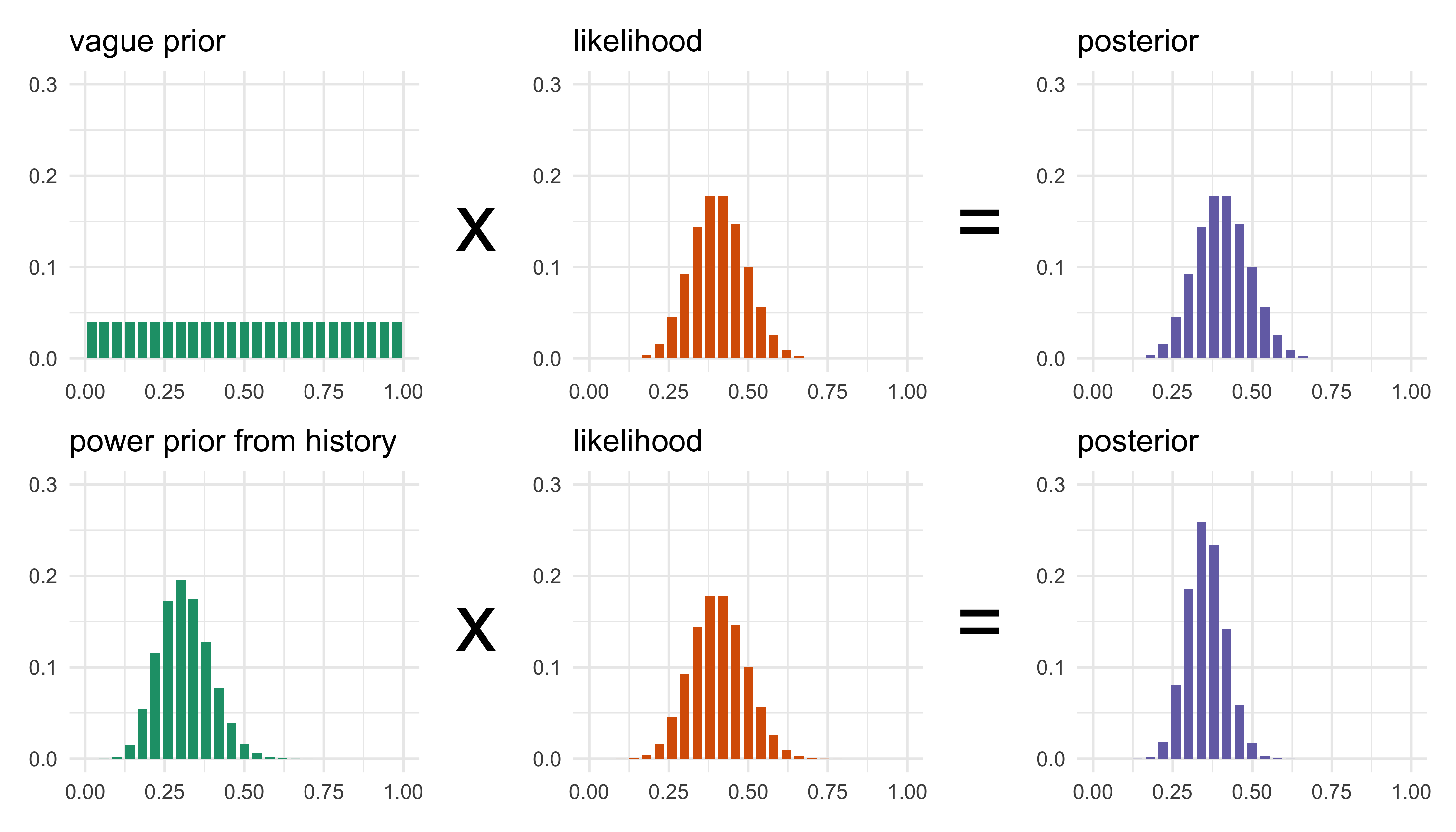
Figure 19.1: Bayes’ rule on a grid of control response rates. Top row: vague Beta(1,1) prior times the likelihood of 12 responders in 30 current controls. Bottom row: power prior from the historical control arm (30/100, weight 0.3) times the same likelihood. Each panel is scaled to sum to one.
Figure 19.1 reads Bayes’ rule as a product of bars. With a vague prior the posterior is the likelihood, with a standard deviation of 0.085. The power prior at \(a_0=0.3\) adds the equivalent of 32 patients to the 30 current controls (ESS \(a_0 n_h+2\)), and the posterior narrows to a standard deviation of 0.06 and moves from 0.41 towards the historical 0.30, to 0.35. The narrowing is the gain, and the shift is the risk: the current data say 40% and the posterior is pulled down by an amount the trial cannot verify. The larger the gap between the historical and the current rate, the more the borrowed bars mislead, and Table 19.3 (and the drift scenarios in Section 19.8) put numbers on what that costs in type I error.
A natural improvement is to treat \(a_0\) as unknown with its own prior, so that the data choose it. This runs into a technical difficulty: the prior in Equation 19.3 as written has a normalizing constant that depends on \(a_0\), and ignoring it makes the posterior favor small \(a_0\) in a way that has nothing to do with agreement between the datasets. The normalized power prior divides by the constant, \[
\pi(\theta, a_0 \mid D_h) = \frac{L(\theta\mid D_h)^{a_0}\,\pi_0(\theta)}{\int L(\theta\mid D_h)^{a_0}\,\pi_0(\theta)\,d\theta}\;\pi(a_0),
\tag{19.4}\] and then the marginal posterior of \(a_0\) increases when the current data resemble the historical data and decreases when they do not. The normalized power prior is due to Duan, Ye, and Smith (2006) and Neuenschwander, Branson, and Spiegelhalter (2009), and M.-H. Chen and Ibrahim (2006) relate it to hierarchical models. For FDA a fixed \(a_0\) is a static method, and a random \(a_0\) updated by the data is a dynamic one (the draft also lists supervised power priors, a term we do not use again). The cost of dynamic methods is more parameters to specify, including the prior on \(a_0\), and an operating characteristic that has to be simulated.
A rare-disease trial: choosing \(a_0\) by the marginal likelihood
A fixed \(a_0\) is a judgment. The data can say something about it, and the simplest way to see how is a small example. Consider a rare metabolic disease. A natural-history study of 40 patients on standard care found 12 responders by a functional criterion (30%). The new trial randomizes 25 patients to the treatment and 15 to standard care, a 5:3 allocation (hypothetical, like the rest of this example) chosen to limit the number of patients on a comparator of doubtful benefit, and observes 14 of 25 responses on treatment and 6 of 15 on control. With uniform priors and no borrowing, the posterior probability that the treatment rate exceeds the control rate is 0.83, an inconclusive result by the 0.975 standard. Table 19.2 shows what the power prior adds.
Table 19.2: Rare-disease trial (14/25 treated, 6/15 control) with a power prior from 12/40 historical controls. The control size, excluding the reference prior, is 15 + 40 a0. The second probability is that the treatment rate exceeds the control rate by more than 0.10.
a0
Control size (excluding reference prior)
Pr(pT > pC)
Pr(pT - pC > 0.1)
0.00
15
0.830
0.619
0.25
25
0.918
0.743
0.50
35
0.951
0.803
1.00
55
0.974
0.859
At \(a_0=0.5\) the control sample is more than doubled and the probability of benefit reaches 0.95. Whether that borrowing is justified is a question about the current controls, and the data speak to it through the marginal likelihood of the current control data as a function of \(a_0\), \[
m(a_0)=\frac{B\bigl(1+a_0y_h+y_c,\;1+a_0(n_h-y_h)+n_c-y_c\bigr)}{B\bigl(1+a_0y_h,\;1+a_0(n_h-y_h)\bigr)},
\tag{19.5}\] with \(B\) the beta function. It measures how well the historical controls predicted the current ones.
Here the current control rate is 6/15, or 40%, close to the historical 30%, and \(m\) is largest at \(a_0=\) 1: full borrowing is supported, with \(m(1)/m(0)=\) 2.3. Had the current controls responded 11 times in 15 (73%), the maximum would move to \(a_0=\) 0 and the trial would stand on its own data. This is an empirical Bayes choice and it is crude, because fifteen patients are asked to judge a disagreement, and the maximizer \(a_0=1\) at a boundary says “no evidence against full borrowing”, not “the populations are the same”. It captures the logic of the commensurate and robust-mixture priors of Section 19.5 and Section 19.6: borrow when the sources agree and stop when they conflict. It does not remove the need for the drift simulation of Section 19.8, because a regulator will ask what the design concludes if the true control rate is 45%, not 30%. Real instances of borrowing from natural-history and earlier-trial controls are told in Section 19.17. Before relying on a source like the 12 of 40 above, check it against the DIA roadmap’s criteria for the quality and comparability of historical controls (Ghadessi et al. 2020), and expect the review division to read it against the rare-disease guidance, which reserves external controls for specific circumstances (U.S. Food and Drug Administration 2023c).
19.5 Commensurate priors
Hobbs, Carlin, Mandrekar and Sargent (2011) put the question of agreement into a parameter of its own (Hobbs et al. 2011) (the paper treats Gaussian data, and the extension to generalized linear models, the case the binary examples of this chapter need, is in Hobbs, Sargent, and Carlin (2012)). Write \(\eta_c\) for the current parameter and \(\eta_h\) for the historical one (for binary data, the logits \(\eta_c=\operatorname{logit}p_c\) and \(\eta_h=\operatorname{logit}p_h\), so that the normal prior is placed on the logit scale). The commensurate prior says \[
\eta_c \mid \eta_h, \tau_c \sim N(\eta_h,\; 1/\tau_c),
\tag{19.6}\] where the commensurability parameter\(\tau_c\) is a precision, with its own prior, typically a spike-and-slab or a discrete mixture that allows a large value (near agreement) and a small value (near independence). Large posterior \(\tau_c\) means the current data support the claim that the two parameters are close, and the historical data count heavily. Small posterior \(\tau_c\) means they do not, and the historical data are down-weighted. In this form the method looks like a hierarchical model with two groups, but there is an important difference in how the historical group is used. In the two-stage version the historical posterior is held fixed and the direction of borrowing is one way, which is the way a regulator thinks about an earlier trial that has already been reported. In the fully Bayesian joint model, information flows both ways through the commensurability parameter.
Hobbs and colleagues also give a version in which the commensurate model sits on a power prior, so that the two ideas, discounting and agreement, are combined. In applications there is a practical issue the original paper discusses: a method that learns agreement from a small current control arm has little to learn from, and so in a small trial the commensurate prior behaves much like a static one with weights fixed by the prior on \(\tau_c\).
19.6 Meta-analytic-predictive priors and robust mixtures
Often there is not one historical control arm but several, from different trials. The meta-analytic-predictive (MAP) prior of Neuenschwander and colleagues (2010) does a random-effects meta-analysis of the historical control rates, using the hierarchical model of Equation 19.1, and then takes the predictive distribution of the control parameter in a new trial as the prior (Neuenschwander et al. 2010). The predictive distribution is wider than the meta-analytic mean because it includes the between-trial variation \(\tau_b\): even if the historical trials were estimated without error, a new trial’s control rate would differ from their average by about \(\tau_b\). This is the logic of an exchangeable new trial, and it is the reason a MAP prior does not become more informative than the heterogeneity warrants however many historical patients there are.
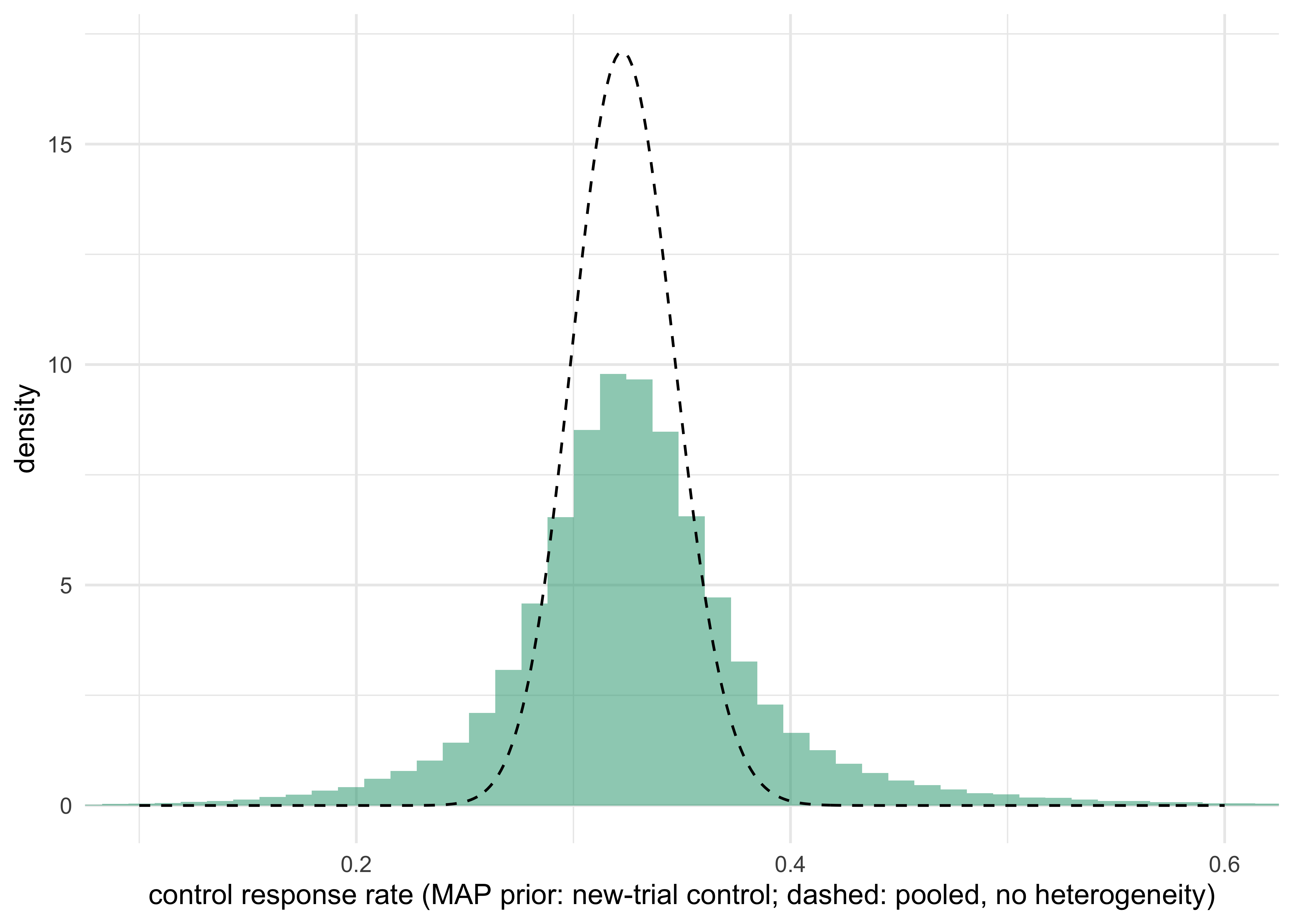
Figure 19.2 shows this with four illustrative historical control arms (80, 100, 70 and 150 patients, 400 in total). The calculation is a normal-normal random-effects model on the logit scale, with a half-normal prior with scale 0.5 on \(\tau_b\), and the predictive distribution is converted to a Beta prior by matching mean and variance.
Code: MAP prior from four historical control arms
q <-quantile(mp$samples, c(0.025, 0.5, 0.975))
Show the R code
x <-seq(0.1, 0.6, length.out =400)pooled <-data.frame(x = x, d =dbeta(x, 1+sum(yh_trials), 1+sum(nh_trials) -sum(yh_trials)))ggplot() +geom_histogram(aes(x = mp$samples, y =after_stat(density)), bins =80, fill ="#1B9E77", alpha =0.5) +geom_line(data = pooled, aes(x, d), linetype ="dashed") +coord_cartesian(xlim =c(0.1, 0.6)) +labs(x ="control response rate (MAP prior: new-trial control; dashed: pooled, no heterogeneity)", y ="density") +theme_minimal()
Figure 19.2: Meta-analytic-predictive prior for the control response rate in a new trial (histogram) compared with the pooled-historical posterior that ignores between-trial variation (dashed). Four illustrative historical arms.
The MAP prior has median 0.326 and 95% interval (0.212, 0.471), with posterior mean \(\tau_b\) of 0.18, and its Beta approximation is Beta(18.8, 38.2). The MAP prior is worth about 57 patients, although 400 patients contributed. The pooled analysis, which ignores between-trial variation, would claim a prior effective sample size of 402 (the 400 historical patients plus the 2 patients of the Beta(1, 1) reference prior). The difference is the between-trial variation, and it is the most important number a regulator can ask for, since it quantifies how much a new trial’s control arm can be expected to differ from the old ones.
A MAP prior is still an exchangeability assumption: it assumes that the new control rate is another draw from the same distribution as the historical ones. If the new trial differs systematically, because standard of care changed or the population is different, the MAP prior is confidently wrong. Schmidli and colleagues (2014) proposed protecting against this with a robust MAP prior, a mixture of the MAP prior and a vague prior (Schmidli et al. 2014): \[
\pi_{\text{rob}}(\theta) = w\,\pi_{\text{MAP}}(\theta) + (1-w)\,\pi_{\text{vague}}(\theta).
\tag{19.7}\] The conjugate update of a mixture is a mixture of conjugate updates, with the weights multiplied by the marginal likelihood of the current data under each component. If the current control data look like the MAP prior, the weight stays on the informative component. If they do not, the weight moves to the vague component and the posterior reverts to the current data (Schmidli et al. 2014). The weight \(1-w\) on the vague component is a choice made at the design stage; values of 0.1 to 0.5 are our working range, not a figure taken from the literature on robust priors. The mixture weight after the data are in plays the role of the commensurability parameter in the previous section, and it is the quantity to report: it says how much of the final answer comes from outside the trial. For production use, the R package RBesT (on CRAN) fits MAP priors by MCMC, approximates them by mixtures of conjugate distributions, and computes robust versions and operating characteristics (Weber et al. 2021); the chunks in this chapter use a simpler normal-normal approximation from bayestrials so that every step is visible. The belimumab pediatric analysis (Section 19.17.2) is the clearest regulatory example of a robust mixture prior.
Let the informative component be Beta\((a,b)\) and the vague one Beta\((1,1)\), with prior weights \(w\) and \(1-w\). After \(y\) successes in \(n\) current control patients, the posterior weight on the informative component is proportional to \(w\,B(a+y,b+n-y)/B(a,b)\), against \((1-w)\,B(1+y,1+n-y)\). The ratio of the two marginal likelihoods is a Bayes factor between a sharp and a diffuse prior. For small \(n\) it takes a large discrepancy to change the Bayes factor by much, because both components assign comparable marginal likelihood to a wide range of \(y\). The weight starts to move only when \(\hat\theta\) is more than a couple of standard errors, \(\sqrt{\theta(1-\theta)/n}\), from the informative component’s mean. In a control arm of 30 patients the standard error is about 0.08, so a true rate 0.10 above the historical rate is within two standard errors and the weight barely moves. This is not a defect of the method. It is the statement that 30 patients cannot tell 30% from 40%, and therefore that dynamic borrowing in a small trial offers weak protection against moderate drift. The simulation below shows the consequence.
19.7 How much does the borrowed information weigh? Effective sample size and conflict
Chapter 8 defined the effective sample size of a prior, and its best known definition is that of Morita, Thall and Mueller (Morita, Thall, and Müller 2008). Definitions differ and give different numbers for the same prior, so a request for the “ESS” should be answered with the definition stated. For borrowing it is the central summary, and FDA asks for it: the draft guidance defines ESS as “a measure of the information in a probability distribution in terms of the equivalent number of patients in the target population”, asks that it be reported across the plausible range of outcomes, with its maximum and its mean, and asks for the ratio of prior ESS to trial size (U.S. Food and Drug Administration 2026). For a static prior the ESS is a number. For a dynamic prior it is a function of the observed current data: the ESS is high when the current control agrees with the historical one and falls when it does not.
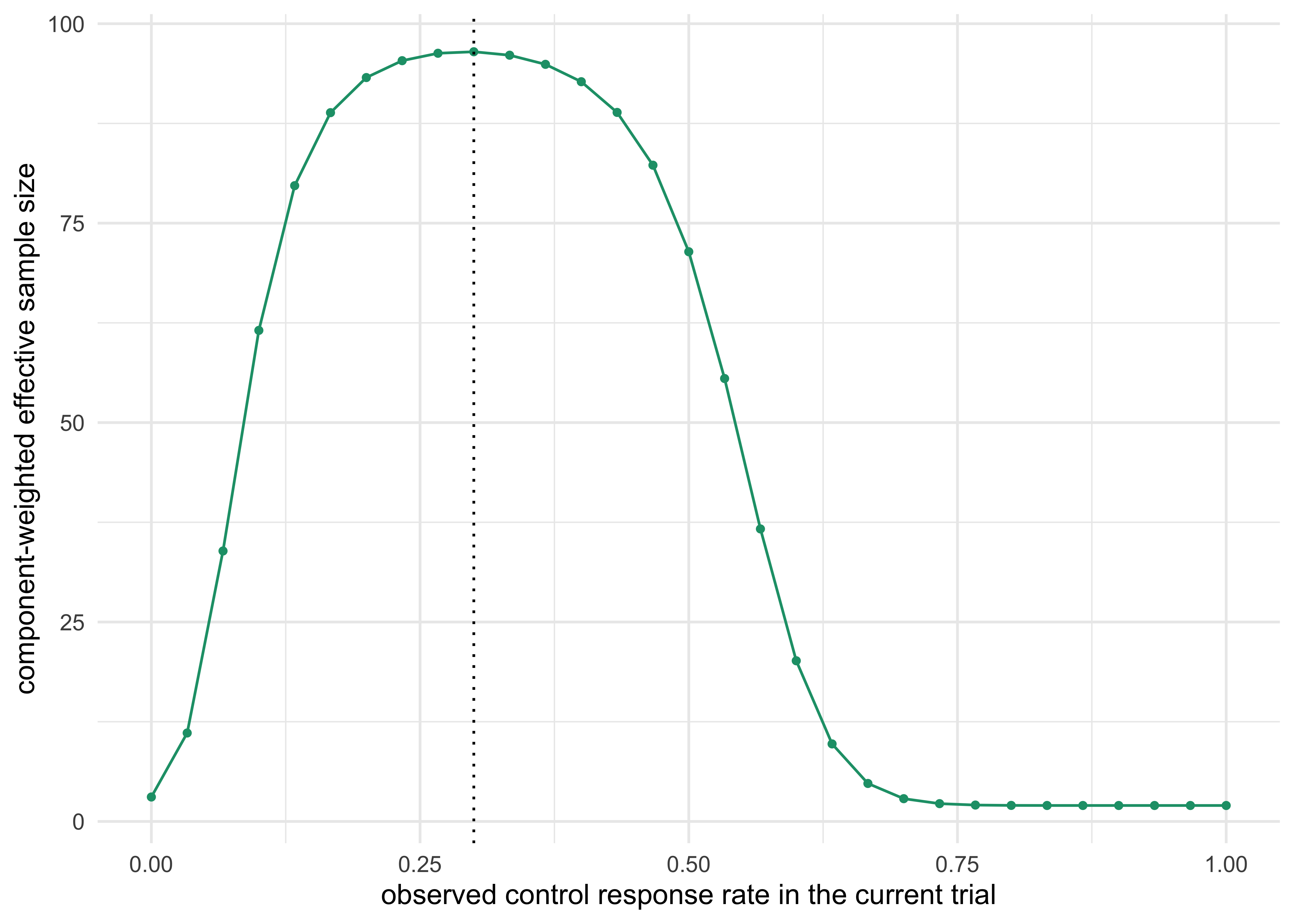
For a robust mixture there is no unique patient-equivalent ESS. A simple convention, used here, is the component-weighted ESS: the posterior weight on each component times that component’s ESS (102 for the informative Beta\((31,71)\), 2 for the vague Beta\((1,1)\)), summed over the two components. Other conventions give different numbers. Figure 19.3 shows it for the example used in the rest of the chapter: a historical control arm of 100 patients with 30 responders, and a current control arm of 30 patients, with a robust prior that puts weight 0.8 on the historical-data Beta\((31,71)\) and 0.2 on Beta\((1,1)\).
Show the R code
yc <-0:ncd <-data.frame(rate = yc / nc, ess =borrow_ess_robust(yc, nc, yh, nh))ggplot(d, aes(rate, ess)) +geom_line(colour ="#1B9E77") +geom_point(colour ="#1B9E77", size =1) +geom_vline(xintercept = yh / nh, linetype ="dotted") +labs(x ="observed control response rate in the current trial", y ="component-weighted effective sample size") +theme_minimal()
Figure 19.3: Dynamic (component-weighted) effective sample size of the robust prior as a function of the number of responders in the current control arm of 30. The historical control is 30/100.
At the historical rate (9 of 30) the weight on the historical component is 0.94 and the borrowed ESS is about 96. At 12 of 30, which is an observed rate ten percentage points above the historical one, the weight is still 0.91. At 15 of 30 it is 0.69, and at 18 of 30 it has fallen to 0.18. The method protects against a gross conflict and does very little against a moderate one.
Prior-data conflict is the general name for this problem: the current data are unlikely under the prior. Two practical diagnostics are used. The first is a prior predictive check: compute the probability, under the prior, of data at least as extreme as the observed control data (a Box p-value), and report it. The second is the weight on the vague component or the posterior of \(a_0\) or \(\tau_c\). Neither detects conflict that the current data are too small to see. The FDA draft asks sponsors to explore prior-data conflict in the design simulations, including a scenario with no effect in the target population (U.S. Food and Drug Administration 2026).
19.8 What borrowing costs: type I error and power under drift
Now the central calculation. Take a two-arm trial with a binary endpoint, with 60 patients on the new treatment and 30 on control (2:1 randomization, so that a smaller concurrent control arm is accepted in return for borrowing). The historical control arm has 100 patients and 30 responders. The decision rule is the one the FDA draft uses, \(\Pr(\delta>0 \mid \text{data}) > c\) with \(\delta=p_1-p_0\) and \(c=0.975\), with a Beta\((1,1)\) prior on the treatment arm. The control arm gets one of four priors:
No borrowing: Beta\((1,1)\).
Full pooling: Beta\((31,71)\), the historical arm added as if it were current.
Power prior, \(a_0=0.3\): Beta\((10,22)\).
Robust MAP-type mixture: 0.8 Beta\((31,71)\) + 0.2 Beta\((1,1)\), with weights updated by the data.
We then ask what happens when the true control rate in the current trial is not the historical 30% but \(0.30+d\), for drift\(d\) between \(-0.15\) and \(+0.20\). For type I error the true treatment rate equals the true control rate. For power the true treatment effect is 0.20 above the control rate. The calculation is exact: the number of responders in each arm is binomial, the decision is a function of the two counts, and the rejection probability is a double sum with no Monte Carlo error.
Code: exact operating characteristics of four borrowing methods under drift
rownames(t1) <-rownames(pw) <- drifts
Show the R code
long <-function(m, lab) data.frame(drift =rep(drifts, ncol(m)), prob =c(m), method =rep(colnames(m), each =nrow(m)), what = lab)d <-rbind(long(t1, "Type I error"), long(pw, "Power"))ggplot(d, aes(drift, prob, colour = method)) +geom_line() +geom_point(size =1) +geom_hline(data =data.frame(what ="Type I error", y =0.025), aes(yintercept = y), linetype ="dashed") +facet_wrap(~what, scales ="free_y") +scale_colour_brewer(palette ="Dark2") +labs(x ="drift: true current control rate minus 0.30", y =NULL, colour =NULL) +theme_minimal() +theme(legend.position ="bottom")
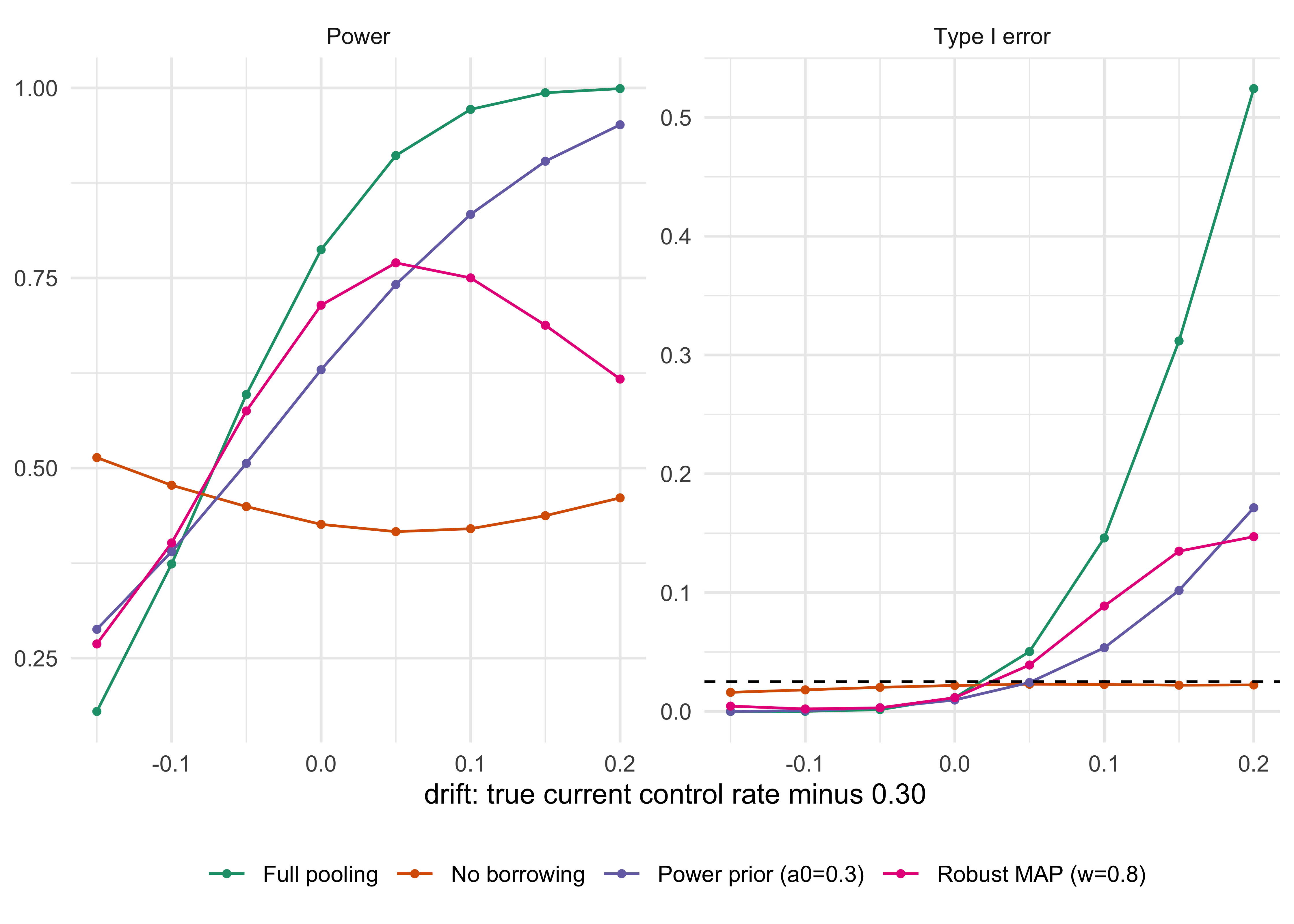
Figure 19.4: Type I error (left) and power (right) of four ways of handling a historical control arm (30/100), as the true current control rate drifts from the historical 30%. Trial: 60 treated, 30 control, rule Pr(p1 > p0 | data) > 0.975. Dashed line: 0.025.
Figure 19.4 plots the whole range, and Table 19.3 reads the numbers that matter off the simulation above.
Table 19.3: Selected operating characteristics from the simulation above (exact enumeration).
True control rate
No borrowing
Full pooling
Power prior
Robust MAP
0.25 (drift \(-0.05\)): power
0.449
0.597
0.506
0.575
0.30 (no drift): type I error
0.022
0.012
0.010
0.012
0.30 (no drift): power
0.426
0.787
0.629
0.714
0.40 (drift \(+0.10\)): type I error
0.023
0.146
0.054
0.089
0.40 (drift \(+0.10\)): power
0.420
0.972
0.834
0.750
0.50 (drift \(+0.20\)): type I error
0.022
0.524
0.171
0.147
Four features of this table are the content of the chapter.
Without drift, borrowing buys power. At the historical rate, full pooling raises power from 0.43 to 0.79 with the same 90 patients, and the type I error is below 0.025 (it is conservative because the decision threshold has not been recalibrated for the borrowed information). The saving is real: it would take a no-borrowing trial with roughly 170 control patients, rather than 30, to match this power (computed with the same exact enumeration and 60 treated patients). The power prior at \(a_0=0.3\) and the robust prior sit in between.
With drift upward, borrowing inflates the type I error, and the inflation is large. If the true control rate is 40% instead of 30%, the Bayesian rule that was conservative at \(d=0\) rejects a true null 14.6% of the time under full pooling, 5.4% under the power prior and 8.9% under the robust prior. At a 20 point drift, full pooling rejects 52% of the time. Nothing is wrong with the arithmetic: the rule “is the treatment rate above the posterior control rate” is correctly computed, and the posterior control rate is anchored at the wrong value. The false positive arises because the historical control appears worse than the treatment, which is exactly the signature of a successful drug.
Without borrowing the type I error does not move. The first column is nearly flat, between 0.016 and 0.023 for every drift. This is the property the traditional design buys by discarding prior data: validity does not depend on any assumption about the past.
The same drift that inflates type I error gives spurious power. The columns for full pooling and the power prior at \(d=+0.10\) show power of 0.97 and 0.83, but this is a mixture of a real effect and an artifact, and a sponsor cannot tell which from the trial. Conversely, at \(d=-0.15\) (the current control rate is 15 points lower than history) full pooling loses power, falling from 0.79 at no drift to 0.18, against 0.51 without borrowing: the posterior control rate is pulled up towards the old 30%, which hides a real treatment effect. Drift in one direction costs type I error and drift in the other costs power. Neither is controlled by the trial.
The robust prior is not a cure. At a ten point drift it still has a type I error of 0.089, higher than the power prior’s 0.054, and only at a twenty point drift (0.147 against 0.171) does it start to protect.
Viele and colleagues compared pooling, power priors and hierarchical borrowing in simulations of this kind and found, as here, that the gain from borrowing is lost or reversed when the current control rate drifts, and that dynamic methods protect only in part (Viele et al. 2014). Galwey argues that, unless a strong assumption is made about the degree of discounting, dynamic borrowing may give little or no gain over using the current data alone, and recommends comparing the consequences of a range of assumptions (Galwey 2017); for a control arm of 30 this agrees with the technical note above. When there is a single historical study, as in the example here, Röver and Friede treat the discount as shrinkage estimation in a Bayesian random-effects meta-analysis of two studies, and illustrate it with a trial and a clinical registry in Creutzfeldt-Jakob disease (Röver and Friede 2020).
What the regulator does with this
In the settings studied by Kopp-Schneider and colleagues, borrowing cannot improve power over an optimal current-data test while preserving strict conditional type I error control given the historical data (Kopp-Schneider, Calderazzo, and Wiesenfarth 2020). Recalibration can restore control, but may remove the gain. So the claim “type I error at most 0.025 over every drift” is available only for a recalibrated rule, and for the uncalibrated rules above inflation at some drift is unavoidable: a rule that is conservative when the historical rate is right gives up something when it is wrong. The FDA draft recognizes this. For designs with borrowing, “this default success criterion may not be applicable or appropriate”, and the sponsor should agree an alternative with the Agency (U.S. Food and Drug Administration 2026). The draft says that it does not recommend using type I error inflation as the measure of how much has been borrowed, because it regards that as philosophically inconsistent with having chosen to borrow, and observes that dynamic methods already reduce borrowing near the null (U.S. Food and Drug Administration 2026). What it asks for instead:
the ESS of the prior and the ratio of prior ESS to the trial’s size, over the range of plausible data;
simulations of prior-data conflict, including a scenario with no effect in the target population (that is the type I error row of the table above, for a chosen set of drift values);
sensitivity analyses that vary the strength of borrowing;
justification that the source and target are relevant: same estimand, comparable standard of care and population, patient-level data where possible, and a pre-specified rule for including sources so that the sponsor cannot pick favorable studies.
The table above is the shape of the simulation report. The one number to add to it is the range of drift that the sponsor believes is plausible and the type I error at the edge of that range. A sponsor who can say “we think the control rate in 2027 lies between 0.25 and 0.35, and at 0.35 our type I error is 0.04” has stated what is being bought and what it costs, and the regulator can negotiate on that basis. A sponsor who reports only the no-drift column has not.
Two protective devices are also in use. A cap on borrowing limits the ESS from the historical source to a fraction of the current trial, such as 30% to 50% (an illustrative range, not a regulatory figure), so that the current data always dominate. A recalibrated threshold raises \(c\) until the type I error at no drift, or at a pre-agreed drift, is at most 0.025, which gives up part of the power gain. Both are choices to put to the Agency early, as FDA recommends for any informative prior.
TipIn the protocol: borrowing from a historical control
State, before the historical data are examined by the sponsor’s statisticians where possible: (1) the source trials and the pre-specified criteria that selected them; (2) the estimand in the historical and current trials and any differences in the definition of response or event; (3) the discounting method, the parameters (for example \(a_0\), \(w\), or the prior on \(\tau_b\)) and the reason for each; (4) the prior ESS and its ratio to the planned control arm; (5) the simulation scenarios, with drift values stated as ranges, and the type I error and power at each; (6) a primary analysis with borrowing and a sensitivity analysis without it, and what happens if they disagree; (7) who sees the current control data when, so that the borrowing parameters are not tuned after the data are seen.
19.9 Traditional versus Bayesian: side by side
Conventional standalone design
Bayesian borrowing
Role of prior data
Sets the design alternative, control rate and \(n\); absent from the analysis
Enters the analysis through a prior on the control parameter
Control arm
Concurrent and randomized, full size
Concurrent, possibly smaller (for example 2:1), supplemented by external information
Validity claim
Type I error at most 0.025 at every null value, whatever the past
No general 0.025 guarantee for the uncalibrated rules: report error rates over the justified drift range, and calibrate over that range if a 0.025 guarantee is claimed (recalibration can remove the power gain)
Main risk
A larger or longer trial than the history suggests is necessary
Bias from a mismatched source, undetectable from a small control arm
Report
p-value, confidence interval
Posterior probability, prior ESS, simulations over conflict
A common disease with a feasible randomized trial, where external controls are not needed
A rare disease or pediatric population where a full concurrent control is infeasible, with strong evidence that the source applies
Where the two agree: with \(a_0=0\), or a vague prior, the Bayesian design is the traditional one in a different notation and (up to the tail calculation) gives the same decision. In a trial large enough that the borrowed ESS is small relative to the trial, the two also agree in practice. Where traditional is the better choice: when a randomized comparison of full size is feasible and the question is the effect of the drug now, the borrowing buys little and risks something.
19.10 Pediatric extrapolation and ICH E11A
Pediatric trials are the setting where borrowing is most often justified, because enrollment is small and withholding treatment from children is difficult ethically. The ICH E11A guideline on pediatric extrapolation, adopted at Step 4 in August 2024, sets out a general approach (International Council for Harmonisation 2024). It asks for a pediatric extrapolation plan with three parts: an assessment of how similar the disease, the drug’s pharmacology and the response to treatment are in the source (adult) and target (pediatric) populations, using whatever is known about the mechanism; a description of the gaps and uncertainties; and a plan for the data to be generated in children, which can range from PK and safety only (full extrapolation of efficacy) to a reduced efficacy trial to a full one. The more similar the populations, the less pediatric data are needed. Bayesian borrowing is one of the quantitative tools that the guideline allows for the middle case, in which adult data are used to inform the pediatric efficacy analysis, and the guideline emphasizes that the same evidence-based judgment of similarity should come first and the statistics second. The intravenous belimumab program in pediatric lupus, analyzed with a robust mixture prior and a tipping-point analysis over the borrowing weight, is described in Section 19.17.2. The FDA framework for extrapolating adult data to children is described by Dunne et al. (2011), and Bayesian modeling for it by Gamalo‐Siebers et al. (2017). For rare diseases generally, FDA’s final guidance of December 2023 says that Bayesian methods may inform pediatric investigations through incorporation of adult data (U.S. Food and Drug Administration 2023c).
The FDA Bayesian draft gives pediatric extrapolation as a core use of an informative prior and names empagliflozin and linagliptin in pediatric type 2 diabetes as examples where Bayesian analyses were supportive (U.S. Food and Drug Administration 2026). It draws two practical points. First, undiscounted adult data would often overwhelm a small pediatric sample, so a prior centered on the adult effect with an inflated variance, representing the possibility that children respond differently, is often more reasonable than pooling. Second, the sources can be related in several ways: equal relevance (adolescents enrolled with adults), exchangeability (a hierarchical model across age strata after adjusting for known effect modifiers), a bias parameter (the pediatric effect equals the adult effect plus an unknown shift), and functional dependence (a pharmacometric model predicting the pediatric effect from adult data and exposure). The bias-parameter form is the one that fits the discount most naturally: if the pediatric effect is \(\theta_p=\theta_a+b\) with \(b\sim N(0,\omega^2)\), then the adult data enter the pediatric prior with variance \(\sigma_a^2+\omega^2\), and the sponsor’s judgment of pediatric similarity is the number \(\omega\). With a large \(\omega\) the adult data contribute little. With \(\omega=0\) they are pooled. The protocol, in effect, writes down \(\omega\) and defends it with the pharmacology.
The design consequence is the same as in the simulation above. Drift in this setting is “the pediatric effect is not the adult effect”, and its plausible range is a clinical judgment about physiology, not a statistical estimate. The simulation of conflict should therefore cover scenarios in which children respond less well than adults, including no effect, and say what the pediatric trial would conclude.
A numerical example shows the bias-parameter form with a mixture prior. Let \(\theta_A\) be the adult log odds ratio, estimated as \(-0.5\) with standard error \(0.08\), and let \(\theta_P\) be the pediatric effect. A pediatric trial of modest size gives \(\hat\theta_P=-0.35\) with standard error \(0.30\). The prior is \[
\theta_P\sim w\,N(\hat\theta_A,\,0.08^2+\omega^2)+(1-w)\,N(0,1),
\tag{19.8}\] where \(\omega\) is the allowed adult-pediatric difference and \(w\) the prior probability that extrapolation is valid.
Show the R code
pm <-borrow_pediatric_mixture(thetaA =-0.5, seA =0.08, tau =0.15, w =0.7, est =-0.35, se =0.3)pm2 <-borrow_pediatric_mixture(est =-0.05)
With \(w=0.7\) and \(\omega=0.15\), the posterior weight on the informative component rises to 0.87, because the pediatric estimate is consistent with the adult one, and the posterior probability of benefit, \(\Pr(\theta_P<0\mid\text{data})\), is 0.98. The pediatric trial alone gives 0.88. The mixture is a weak safeguard in a trial this small, and the example shows it: if the pediatric estimate had been \(-0.05\) instead, the weight on the informative component would fall only to 0.75, and the probability of benefit would still be 0.89 against 0.57 for the trial alone. With a standard error of 0.30 the pediatric data cannot tell the two components apart, so the answer is mostly the prior, which is why the simulation of conflict above must include scenarios in which children respond less well. The prior weight \(w\) is the honest summary of the clinical judgment about similarity in the E11A extrapolation plan, and writing it down is what lets a review committee debate it.
19.11 Noninferiority with borrowed information
A noninferiority trial is a borrowing problem from the start. Its margin comes from the control’s effect in earlier placebo-controlled trials, and its validity rests on the constancy assumption that this effect still holds (Section 4.9; FDA 2016 (U.S. Food and Drug Administration 2016); ICH E10 (International Council for Harmonisation 2000)). The traditional analysis uses the historical data once to fix a margin and then treats the margin as known. The Bayesian analysis can state the same thing as a model.
Take a difference in event rates \(\theta=p_N-p_C\) (new minus control, events bad), noninferior if \(\theta<M\). Suppose a trial estimates \(\hat\theta=0.01\) with standard error \(0.015\) and the margin is \(M=0.04\). The upper limit of the two-sided 95% interval is \(0.01+1.96\times0.015=\) 0.0394, just under the margin, so the traditional test succeeds. Table 19.4 gives the posterior probability of noninferiority under three priors.
Table 19.4: Posterior probability of noninferiority, estimate 0.01, standard error 0.015, margin M = 0.04. Skeptical prior: N(M, 0.02^2). Enthusiastic prior: N(0, 0.01^2). Flat: improper uniform.
Prior
Posterior mean
Pr(theta < M)
Flat
0.010
0.977
Skeptical, N(M, 0.02^2)
0.021
0.945
Enthusiastic, N(0, 0.01^2)
0.003
>0.999
Under the flat prior the posterior probability is one minus the one-sided p-value, 0.977, as it must be (Section 4.10). The skeptical prior, centered at the margin, is the natural regulatory prior for noninferiority: it represents a reviewer who thinks the new drug is as likely to be unacceptably worse as acceptably close. Under it the probability is 0.945, below the 0.975 that the traditional test implicitly demands. The prior is doing visible work, and the reviewer and the sponsor can argue about its standard deviation instead of about a p-value.
Margin synthesis
Regulatory practice preserves a fraction \(f\) of the control’s effect against placebo, \(\delta_{CP}\), estimated from the historical trials as \(N(d,s_{CP}^2)\). The fixed-margin approach takes the lower 95% limit of \(\delta_{CP}\), multiplies by \(1-f\) (the loss of effect that is allowed), and uses the result as the margin \(M_2\). The synthesis alternative asks directly for the posterior probability that the new drug retains at least the fraction \(f\), \[
\Pr\bigl(\theta_{NC}<(1-f)\,\delta_{CP}\mid\text{data}\bigr),
\tag{19.9}\] with \(\theta_{NC}\) the new-minus-control difference (events bad). The network meta-analytic-predictive approach of Schmidli, Wandel and Neuenschwander is the hierarchical-model counterpart: it combines the historical trials with data on the active control and on placebo, together with the noninferiority trial, in a network meta-analysis, and predicts the effect of the test treatment against placebo in the noninferiority trial while carrying the between-trial variability of all parameters (Schmidli, Wandel, and Neuenschwander 2013). Prior-data conflict can be handled by a robust mixture, as in Section 19.6. The synthesis method is usually credited to Rothmann et al. (2003), with an earlier method for comparison to placebo in active-control trials in Hasselblad and Kong (2001), its preservation-of-effect interpretation and error properties are in Snapinn and Jiang (2008), a Bayesian formulation is in Simon (1999), and the constancy assumption is discussed by Fleming (2008). The fixed-margin approach reduces the historical estimate to a single conservative number, the lower confidence limit, and so builds in a deliberate conservatism; the synthesis carries the full uncertainty of the historical estimate into the comparison. Both rest on the constancy assumption, and the synthesis makes it visible: if care has improved since the historical trials and the control’s effect has shrunk, discounting by a power prior with \(a_0<1\) would only widen the distribution of \(\delta_{CP}\) and leave its center where it was. A shrunken effect has to be modeled directly, for example by shifting or scaling the center of \(\delta_{CP}\) by an attenuation or bias parameter with its own prior, and the retained fraction should be assessed over a range of plausible downward shifts.
Show the R code
sy <-ni_synthesis(est =0.01, se =0.015, d =0.10, s_cp =0.02, f =0.5)sy_hi <-ni_synthesis(est =0.04, se =0.015, d =0.10, s_cp =0.02, f =0.5)
An illustration, with hypothetical numbers: let the historical control effect be a 10-point event reduction with standard error 0.02, and let the sponsor aim to preserve half of it. The fixed margin is half the lower 95% limit, 0.03, tighter than the 0.04 above, and the trial with \(\hat\theta=0.01\) and standard error 0.015 (upper limit 0.039) does not meet it. The synthesis probability of retaining at least half of the effect is 0.987. The two answers differ because the fixed margin spends all of the historical uncertainty at its worst limit and then asks the current trial to clear that limit at 0.025, which is two conservative operations stacked. The synthesis is not automatically more lenient: for a trial with \(\hat\theta=0.04\) the probability of retaining half the effect is only 0.71. Whether a regulator will accept a synthesis rule in place of a fixed margin, and with what threshold, is a question for the protocol and for early discussion with the agency; the 2016 guidance describes both approaches.
19.12 Indirect comparison through a common comparator: the tirzepatide chain
The question a guideline committee asks of SURPASS-CVOT is how much tirzepatide lowers cardiovascular risk compared with no incretin therapy at all. No trial answers it directly: SURPASS-CVOT compared tirzepatide with dulaglutide, and REWIND compared dulaglutide with placebo (Nicholls et al. 2025; Gerstein et al. 2019). The answer has to be assembled, and on the log scale the effects add, \[
\log\mathrm{HR}_{T:P}=\log\mathrm{HR}_{T:D}+\log\mathrm{HR}_{D:P},
\tag{19.10}\] with variances adding if the two estimates are independent. SURPASS-CVOT gave a hazard ratio of 0.92 (95.3% CI 0.83 to 1.01) and REWIND 0.88 (95% CI 0.79 to 0.99).
Table 19.5: Tirzepatide versus placebo, chained through dulaglutide: SURPASS-CVOT (HR 0.92) times REWIND (HR 0.88), with the REWIND variance divided by the power-prior weight a0. Standard errors from the published intervals: 0.0496 and 0.0577.
a0
HR
95% interval
Pr(HR < 1)
1.00
0.81
0.70 to 0.94
0.997
0.50
0.81
0.67 to 0.98
0.987
0.25
0.81
0.63 to 1.04
0.954
0.10
0.81
0.56 to 1.17
0.868
At \(a_0=1\) the chain gives a hazard ratio of 0.81 with interval 0.70 to 0.94. The calculation assumes the constancy assumption again: the dulaglutide effect in REWIND is the dulaglutide effect in the SURPASS-CVOT population. The populations differ. REWIND enrolled patients aged 50 or older, with and without established cardiovascular disease, in 2011 to 2013, whereas SURPASS-CVOT enrolled only patients with established disease, a decade later and on different background therapy. A power prior discounts the REWIND evidence: dividing its variance by \(a_0\) widens the interval and leaves the estimate where it was. At \(a_0=0.5\) the interval is 0.67 to 0.98, and at \(a_0=0.25\) it is 0.63 to 1.04, so the conclusion of a benefit against placebo survives a halving of the weight on REWIND but not a quartering. Reporting the table lets a reader pick the weight, and shows where the conclusion changes.
As in Section 19.4, the discount widens the interval but does not move the center. If the REWIND effect in the SURPASS-CVOT population differs from 0.88, the discount is the wrong correction. The published indirect comparison of Sattar and colleagues addresses exactly this (Sattar et al. 2026). It was prespecified, and it used propensity-score adjustment to select and weight 2055 of the 9901 REWIND participants who resemble the SURPASS-CVOT population, then multiplied the SURPASS-CVOT hazard ratio by the REWIND hazard ratio in that subset. Its primary result is a hazard ratio of 0.72 (95% CI 0.55 to 0.94) for the primary composite against an imputed placebo. That is lower than the simple chain’s 0.81, which is consistent with a larger dulaglutide effect in the REWIND subset with established disease than the overall 0.88 (the paper itself reports a hazard ratio of 0.78, 95% CI 0.61 to 1.01, for the selected REWIND cohort, which is a different quantity from the propensity-weighted indirect analysis). The two answers rest on different assumptions about exchangeability, and the Bayesian formulation lets both be reported: the unadjusted chain with its discount table, and the adjusted analysis with its own uncertainty. Neither is a randomized comparison with placebo. For a regulator, this is the evidence that supports a label discussion or a guideline recommendation, not a primary efficacy claim.
19.13 Borrowing across subgroups: basket trials
A basket trial tests one therapy in several tumor types or biomarker-defined subgroups that share a molecular target. Each basket is small, and the question is which baskets respond. The traditional design runs a separate single-arm test in each basket, with a multiplicity adjustment across them (Chapter 10). The Bayesian design puts the baskets in a hierarchical model, Equation 19.1, so that responses in one basket inform the others. Thall and colleagues (2003) proposed the hierarchical model for phase II trials in diseases with multiple subtypes, and Berry and colleagues (2013) applied it to oncology subpopulations, reporting designs that need fewer patients per subgroup than independent analyses at the same type I error under their scenarios (Thall et al. 2003; Berry et al. 2013). In Polson and Sokolov (2026) the quoted figure is 4 to 7 patients per group fewer than independent analyses. It comes from the scenarios that Berry and colleagues chose themselves, so it shows what the method can achieve and not what it will achieve in a given trial.
The next chunk shows the mechanism with ten baskets of 30 patients each. In the first scenario nine baskets have 12 responders (40%) and one has 3 (10%). In the second all ten have 12.
Code: hierarchical shrinkage across ten baskets
a <-borrow_basket_posterior(c(rep(12, 9), 3), rep(30, 10))b <-borrow_basket_posterior(rep(12, 10), rep(30, 10))
In the all-equal scenario the model estimates a small \(\tau_b\) and every basket’s estimate stays at its observed 40%. The estimate is close to the observed rate because nothing disagrees, and the posterior interval for each basket is narrower than it would be alone. In the outlier scenario, the observed heterogeneity pushes \(\tau_b\) up, so that the nine typical baskets are pulled down from 40% to about 38% by the outlier and the outlier is pulled up from 10% to about 29%. The outlier is moved a lot because it has only 30 patients and the model, informed by nine similar baskets, regards a rate of 10% as probably a low draw. If the outlier is in fact a non-responding tumor type, the model has overstated its response rate by almost three-fold, which is the “estimated worse” warning of the earlier section. The treatment effect in a basket that really does not respond is overestimated, and a decision rule such as \(\Pr(p_k>0.2\mid y)>c\) will, for some true rates, reject more often than it would with independent analyses. The inflation is again the price, and the same remedy applies: calibrate the threshold by simulation, over scenarios in which some baskets respond and others do not, and report the false positive rate for the non-responding baskets in each. FDA’s draft guidance lists basket trials under borrowing across similar diseases or subtypes, and recommends that the sponsor justify exchangeability and to model known effect modifiers, such as biomarker status, explicitly (U.S. Food and Drug Administration 2026). Chapter 20 returns to the master-protocol setting, and Chapter 10 treats the shrinkage idea for endpoints.
Several variants are worth knowing. The calibrated Bayesian hierarchical model (CBHM) of Chu and Yuan (2018a) sets the amount of shrinkage as a function of the heterogeneity seen in the data, so that baskets that agree borrow more. The Bayesian latent subgroup design (BLAST) of Chu and Yuan (2018b) assigns each cancer type to a latent sensitive or insensitive subgroup and jointly models the binary response and a longitudinal biomarker, so that a non-responding tumor type is not averaged with responding ones. The exchangeability-nonexchangeability model (EXNEX) of Neuenschwander et al. (2016) gives each basket a prior probability of belonging to the common group, much as the robust prior does for a single historical control. Other designs monitor exchangeability as data accrue (Hobbs and Landin 2018) or estimate which baskets are exchangeable (Kaizer, Koopmeiners, and Hobbs 2018), and Simon et al. (2016) give a Bayesian basket design. All fit the same template: the amount of borrowing is a parameter, and the operating characteristics under heterogeneity, above all the false positive rate when some baskets do not respond, have to be simulated.
19.14 When borrowing failed: the NSCLC case study
A sponsor deciding whether a fixed-weight power prior is enough can look at a case study that tested it. Struebing and colleagues (2024) built a matched real-world external control arm in first-line non-small cell lung cancer, augmented it with historical-trial data through a fixed-weight power prior, and compared the result with the survival result of the randomized trial whose control arm it replaced (Struebing et al. 2024). The result was a negative one: the augmented external control did not reproduce the randomized result.
The lesson is the one in the simulation, from a real dataset. A power prior with a fixed discount lowers the weight of the historical data but does not change their center. Discounting does not remove differences between the sources, and if real-world patients differ from trial patients in prognostic factors that matching did not capture, the augmented control stays biased. The study is one case and should not be generalized beyond what it shows, but it is the right example to put in front of a team that proposes to replace a concurrent control with a matched external one: matching on measured covariates removes only the measured bias.
19.15 Prognostic covariate adjustment and digital twins
There is a way of using external data that does not borrow outcomes of the control arm and therefore carries no bias risk of this kind. Prognostic covariate adjustment (PROCOVA) builds a prognostic model of the control-arm outcome from external data, such as historical trial data, and then uses each trial participant’s predicted outcome (their “digital twin” prediction under control) as a baseline covariate in the analysis of the randomized trial. The treatment effect is still estimated by comparing the randomized arms, so the analysis remains valid, and the covariate absorbs variation in the outcome, so the variance falls. The EMA’s Committee for Medicinal Products for Human Use adopted a qualification opinion for the method in September 2022, for phase 2 and 3 trials with continuous outcomes (European Medicines Agency, Committee for Medicinal Products for Human Use (CHMP) 2022). The key regulatory feature, as with the covariate adjustment guidance of FDA, is that the model is fixed before the trial starts: with an independently developed, pre-specified score and appropriate analysis and variance estimation, PROCOVA can preserve asymptotic type I error control despite poor prediction, whereas small trials need suitable finite-sample inference (U.S. Food and Drug Administration 2023d; European Medicines Agency, Committee for Medicinal Products for Human Use (CHMP) 2022). Precision gains depend on prognostic performance. What the sponsor gains is variance reduction, which can be converted into a smaller sample size, up to the limit the qualification opinion sets; no assumption about the stability of the control arm over time is made. The contrast to take away is that PROCOVA uses external data to sharpen a randomized comparison, whereas borrowing uses them to replace part of it (Ross et al. 2024).
This is why the method is often the first one to propose to a regulator who is wary of external controls. It gives up less (the randomized control stays) and so buys less than a full borrowing design, but what it buys carries no assumption about drift. It is a special case of the covariate adjustment of Section 5.10, with a single prognostic score as the covariate, and the guidance of FDA and EMA on prespecification and the estimand applies to it.
19.16 Putting it together: a decision guide
The chapter’s methods fall on a line from no use of external information to full reliance on it. A practical ordering for a team choosing among them:
Is a concurrent randomized control feasible? If yes, and the question is the effect of the drug in the current population, use it at full size, or use PROCOVA-type adjustment to raise precision without borrowing. This is the traditional design and it is hard to beat.
If the concurrent control must be small, is there a randomized source for the same control treatment in the same population? If so, a pre-specified dynamic borrowing design (robust MAP or commensurate) is defensible, as in REBYOTA (Section 19.17.1). Report the ESS, the conflict simulations and a sensitivity analysis without borrowing.
If the only sources are non-randomized (registries, real-world data, historical single-arm series)? Follow the FDA external-controls draft: pre-specify, demonstrate comparability, quantify what is borrowed, and treat the result as supportive unless the effect is large and the natural history is predictable (ICH E10). Expect the NSCLC lesson to apply.
Pediatric? Begin with the E11A extrapolation plan. Write the similarity judgment as a number (\(\omega\), \(a_0\), \(w\)), defend it, and simulate the case in which it is wrong.
Subgroups of a disease or baskets? A hierarchical model is natural. Justify exchangeability across baskets, include known effect modifiers, and simulate scenarios with some baskets not responding.
19.17 In practice
Three regulatory cases show what borrowing buys and what it risks. Two more appear earlier in the chapter: the NSCLC external-control study (Section 19.14), where a matched real-world control with a fixed-weight power prior failed to reproduce a randomized result, and the EMA qualification of PROCOVA (Section 19.15), which uses external data to sharpen a randomized comparison without borrowing outcomes.
REBYOTA: dynamic borrowing from a phase 2b study
REBYOTA (RBX2660, fecal microbiota, live-jslm) prevents recurrence of Clostridioides difficile infection after antibiotics, and was approved on 30 November 2022. The sponsor first planned two phase 3 trials of about 300 patients each. After FDA’s July 2013 enforcement discretion on fecal microbiota transplantation made enrollment difficult, it proposed a single phase 3 trial (study 2017-01, PUNCH CD3) plus a Bayesian integration of the earlier phase 2b study 2014-01. FDA wrote that the studies “are generally exchangeable” but not identical, and accepted a Bayesian hierarchical model with dynamic borrowing, in which the extent of borrowing depends on how similar the effect is in both the active and placebo arms (U.S. Food and Drug Administration, Center for Biologics Evaluation and Research 2022). The January 2026 FDA draft guidance cites this as its example of borrowing from a previous trial of the same drug (U.S. Food and Drug Administration 2026).
The success criteria are the interesting part. The sponsor set two thresholds on the posterior probability of superiority as analogues of a one-sided type I error of 0.025 (one adequate and well-controlled trial) and one-sided 0.00125 (a substitute for two trials), each without borrowing. After adjusting for the information fraction actually reached, they were 0.9750338 and 0.9993275. The modified intention-to-treat result was an estimated success rate of 0.71 on RBX2660 against 0.57 on placebo (difference 0.13, computed from unrounded estimates, 95% credible interval 0.02 to 0.24), with posterior probability of superiority 0.991. That met the one-trial threshold and missed the two-trial threshold (U.S. Food and Drug Administration, Center for Biologics Evaluation and Research 2022).
The lesson is about data alignment, not about the model. During the review FDA requested a refined analysis that aligned the success definition, the assessment period (9 weeks in 2014-01 against 8 weeks in 2017-01) and the analysis populations of the old study to those of the new one, so as to improve exchangeability. The sponsor’s primary analysis had also used non-final 2014-01 data, from which six randomized but undosed subjects had been wrongly excluded. Both the specified analysis and the refined one reached the same conclusion. The briefing document gives no borrowing weight or ESS, so the amount borrowed cannot be read from it. For a sponsor, the checklist of Section 19.16 applies: same product, randomized source, pre-specified model, and alignment of definitions before the data are analyzed.
Belimumab in pediatric lupus: a robust mixture and a tipping point
The pediatric trial of intravenous belimumab in systemic lupus erythematosus (C1109, PLUTO) randomized 93 children (92 in the analysis below). At week 52 the SRI-4 response was 28 of 53 (52.8%) on belimumab and 17 of 39 (43.6%) on placebo, an observed difference of 9.2 points with an odds ratio of 1.5 (95% CI 0.6 to 3.5) (Brunner et al. 2020; U.S. Food and Drug Administration, Center for Drug Evaluation and Research 2026). That interval is far too wide to stand alone. FDA recommended a post hoc Bayesian analysis that borrowed from two adult trials (C1056 and C1057) with the same SRI-4 endpoint and the same 10 mg/kg dose (U.S. Food and Drug Administration, Center for Drug Evaluation and Research 2026).
The prior was a robust mixture of the form of Equation 19.7: an informative component built from the adult placebo and 10 mg/kg arms, and a minimally informative component, with borrowing weight \(w\). Instead of fixing one value of \(w\), the analysis was a tipping-point analysis. The posterior probability of efficacy reached at least 97.5% whenever \(w\) was 0.55 or more, and the review division judged such a weight reasonable given a similar disease course, similar pharmacokinetics and similar baseline characteristics (U.S. Food and Drug Administration, Center for Drug Evaluation and Research 2026). The case study stresses that the analysis was post hoc and that future programs should pre-specify it, with the discussion starting before the IND.
The tipping-point analysis is the practical answer to the question “what weight should we use?”. It reports the smallest amount of borrowing that supports the conclusion and leaves the judgment of its plausibility to the clinical and pharmacological evidence, which is the role of \(\omega\) in the pediatric section above.
OPTIMIZER Smart: what a fixed 30% weight buys
The OPTIMIZER Smart System (cardiac contractility modulation, Impulse Dynamics, PMA P180036) was reviewed by an FDA device panel on 4 December 2018 and approved on 21 March 2019 for heart failure patients in NYHA class III with ejection fraction 25 to 45%. The pivotal trial FIX-HF-5C randomized 160 patients 1:1 and was analyzed with a Bayesian model that included “30% fixed borrowing” of data from the 229 patients with ejection fraction above 25% in the earlier FIX-HF-5 study. The primary endpoint was the change in peak VO2 at 24 weeks, and success required a posterior probability above 0.975 (U.S. Food and Drug Administration, Center for Devices and Radiological Health 2019).
Table 13 of the summary of safety and effectiveness gives the result under four ways of handling missing data. With borrowing the posterior probability was between 0.977 and 0.989 in all four, so the success criterion was met. FIX-HF-5C alone gave 0.957 and 0.960 under two of the imputation models, 0.916 for the complete-case analysis and 0.911 with last observation carried forward, below 0.975 in each (U.S. Food and Drug Administration, Center for Devices and Radiological Health 2019). The success of the device therefore depended on the borrowed 30%, and this is the clearest illustration in the book of both sides of borrowing. The borrowed information was worth a decision, which is the gain of the simulation above. It also carries the risk of the same simulation: if the earlier study overstated the effect, the conclusion rests on that overstatement. The FDA device guidance expects the sponsor to show simulated operating characteristics under such discrepancies (U.S. Food and Drug Administration 2010), and the fixed weight is the device analogue of the power prior with \(a_0=0.3\) used in our example.
Key points
A conventional standalone randomized-trial analysis uses prior data to choose the alternative, the control rate and the sample size, and then ignores them in the analysis. This is why its type I error does not depend on the past.
External and historical controls are regarded with caution by ICH E10 and by FDA, MHRA and EMA because of selection, time trends and measurement differences. Pocock’s 1976 criteria are still the checklist. FDA’s externally controlled trials draft (February 2023), the MHRA draft and the EMA concept paper (2025, adopted May 2026) ask for pre-specification and fitness for purpose.
Bayesian methods choose how much to borrow: fixed discount (power prior), estimated heterogeneity (hierarchical model, MAP prior), estimated agreement (commensurate, normalized power prior), or a mixture with a vague component (robust MAP). Static methods fix the borrowing in advance; dynamic ones let the data adjust it.
Effective sample size is the summary of how much of the answer comes from outside the trial. A MAP prior built from 400 historical patients can be worth about 57 patients once between-trial variation is counted.
Borrowing buys power when the historical rate is right (0.43 to 0.79 in the example) and inflates type I error when it is wrong (0.023 without borrowing, 0.146 with full pooling, 0.054 with the power prior and 0.089 with the robust prior at a ten point drift). A control arm of 30 cannot detect a ten point drift well enough for a dynamic method to protect against it.
FDA’s January 2026 draft asks for the prior ESS, simulations of prior-data conflict (including no effect), and sensitivity analyses. It does not recommend using type I error inflation to measure the amount of borrowing.
REBYOTA is the template of a good case: a randomized phase 2b source for the same product, a pre-specified hierarchical model with dynamic borrowing, a posterior of 0.991 that met the one-trial threshold (0.975) but not the two-trial one (0.99933), and a data-alignment fix from FDA. In OPTIMIZER the success criterion (0.975) was met with a fixed 30% borrowing (0.977 to 0.989) and missed without it (0.911 to 0.960). Belimumab in children was supported by a robust mixture prior with a tipping point at borrowing weight 0.55. ICH E11A (August 2024) puts the similarity judgment first in pediatric extrapolation, and Bayesian borrowing second.
Basket trials use hierarchical models to borrow across tumor types, at the price of over-estimating the response in baskets that do not respond. In an NSCLC case study, a matched real-world control augmented with a fixed-weight power prior did not reproduce the randomized result.
PROCOVA uses external data without borrowing outcomes, so the randomized comparison and its type I error are unchanged, and the gain is variance reduction.
NoteDiscussion questions
A sponsor proposes a 2:1 trial with a control arm of 30, borrowing from a historical control of 100 patients with a robust prior. What drift would you want the simulation to cover, who should decide the range, and what type I error at the edge would you accept for a serious but non-life-threatening condition? For a condition with no approved therapy?
The FDA draft recommends against using type I error inflation as the measure of how much a design borrows, yet asks for conflict simulations that include a no-effect scenario. How are these two positions consistent? Where would you draw the line between a legitimate price of borrowing and an unacceptable one?
A MAP prior from four trials has an ESS of 57 while the pooled analysis would give 400. Which of those two numbers would you put in the protocol, and what does the difference tell a clinician about how much a new control arm should be expected to differ from the old ones?
In the pediatric setting, the similarity judgment \(\omega\) is a clinical, not a statistical, number. Who should supply it, when should it be fixed, and what should the sponsor do if the pediatric interim data suggest it was too optimistic?
In a basket trial, nine tumor types respond and one does not. The hierarchical model reports the non-responding type at 29% against an observed 10%. What decision rule and what calibration would you propose so that a regulator would not label the basket “responding” on the strength of the other nine?
Berry, Scott M, Kristine R Broglio, Susan Groshen, and Donald A Berry. 2013. “Bayesian Hierarchical Modeling of Patient Subpopulations: Efficient Designs of Phase II Oncology Clinical Trials.”Clinical Trials 10 (5): 720–34. https://doi.org/10.1177/1740774513497539.
Brunner, Hermine I, Carlos Abud-Mendoza, Diego O Viola, Inmaculada Calvo Penades, Deborah Levy, Jordi Anton, Julia E Calderon, et al. 2020. “Safety and Efficacy of Intravenous Belimumab in Children with Systemic Lupus Erythematosus: Results from a Randomised, Placebo-Controlled Trial.”Annals of the Rheumatic Diseases 79 (10): 1340–48. https://doi.org/10.1136/annrheumdis-2020-217101.
Chen, Ming-Hui, and Joseph G. Ibrahim. 2006. “The Relationship Between the Power Prior and Hierarchical Models.”Bayesian Analysis 1 (3): 551–74. https://doi.org/10.1214/06-BA118.
Chen, Wei-Chen, Chenguang Wang, Heng Li, Nelson Lu, Ram Tiwari, Yunling Xu, and Lilly Q. Yue. 2020. “Propensity Score-Integrated Composite Likelihood Approach for Augmenting the Control Arm of a Randomized Controlled Trial by Incorporating Real-World Data.”Journal of Biopharmaceutical Statistics 30 (3): 508–20. https://doi.org/10.1080/10543406.2020.1730877.
Chu, Yiyi, and Ying Yuan. 2018a. “A Bayesian Basket Trial Design Using a Calibrated Bayesian Hierarchical Model.”Clinical Trials 15 (2): 149–58. https://doi.org/10.1177/1740774518755122.
———. 2018b. “BLAST: Bayesian Latent Subgroup Design for Basket Trials Accounting for Patient Heterogeneity.”Journal of the Royal Statistical Society: Series C 67 (3): 723–40. https://doi.org/10.1111/rssc.12255.
Duan, Yuyan, Keying Ye, and Eric P. Smith. 2006. “Evaluating Water Quality Using Power Priors to Incorporate Historical Information.”Environmetrics 17 (1): 95–106. https://doi.org/10.1002/env.752.
Dunne, Julia, William J. Rodriguez, M. Dianne Murphy, B. Nhi Beasley, Gilbert J. Burckart, Jonca D. Filie, Lisa L. Lewis, et al. 2011. “Extrapolation of Adult Data and Other Data in Pediatric Drug-Development Programs.”Pediatrics 128 (5): e1242–49. https://doi.org/10.1542/peds.2010-3487d.
Fleming, Thomas R. 2008. “Current Issues in Non-Inferiority Trials.”Statistics in Medicine 27 (3): 317–32. https://doi.org/10.1002/sim.2855.
Galwey, Nicholas W. 2017. “Supplementation of a Clinical Trial by Historical Control Data: Is the Prospect of Dynamic Borrowing an Illusion?”Statistics in Medicine 36 (6): 899–916. https://doi.org/10.1002/sim.7180.
Gamalo‐Siebers, Margaret, Jasmina Savic, Cynthia Basu, Xin Zhao, Mathangi Gopalakrishnan, Aijun Gao, Guochen Song, et al. 2017. “Statistical Modeling for Bayesian Extrapolation of Adult Clinical Trial Information in Pediatric Drug Evaluation.”Pharmaceutical Statistics 16 (4): 232–49. https://doi.org/10.1002/pst.1807.
Gerstein, Hertzel C., Helen M. Colhoun, Gilles R. Dagenais, Rafael Diaz, Mark Lakshmanan, Prem Pais, Jeffrey Probstfield, et al. 2019. “Dulaglutide and Cardiovascular Outcomes in Type 2 Diabetes (REWIND): A Double-Blind, Randomised Placebo-Controlled Trial.”The Lancet 394 (10193): 121–30. https://doi.org/10.1016/S0140-6736(19)31149-3.
Ghadessi, Mercedeh, Rui Tang, Joey Zhou, Rong Liu, Chenkun Wang, Kiichiro Toyoizumi, Chaoqun Mei, Lixia Zhang, C. Q. Deng, and Robert A. Beckman. 2020. “A Roadmap to Using Historical Controls in Clinical Trials by Drug Information Association Adaptive Design Scientific Working Group (DIA-ADSWG).”Orphanet Journal of Rare Diseases 15: 69. https://doi.org/10.1186/s13023-020-1332-x.
Hasselblad, Vic, and David F. Kong. 2001. “Statistical Methods for Comparison to Placebo in Active-Control Trials.”Drug Information Journal 35 (2): 435–49. https://doi.org/10.1177/009286150103500212.
Hobbs, Brian P., Bradley P. Carlin, Sumithra J. Mandrekar, and Daniel J. Sargent. 2011. “Hierarchical Commensurate and Power Prior Models for Adaptive Incorporation of Historical Information in Clinical Trials.”Biometrics 67 (3): 1047–56. https://doi.org/10.1111/j.1541-0420.2011.01564.x.
Hobbs, Brian P., and Rodney Landin. 2018. “Bayesian Basket Trial Design with Exchangeability Monitoring.”Statistics in Medicine 37 (25): 3557–72. https://doi.org/10.1002/sim.7893.
Hobbs, Brian P., Daniel J. Sargent, and Bradley P. Carlin. 2012. “Commensurate Priors for Incorporating Historical Information in Clinical Trials Using General and Generalized Linear Models.”Bayesian Analysis 7 (3): 639–74. https://doi.org/10.1214/12-BA722.
Ibrahim, Joseph G., and Ming-Hui Chen. 2000. “Power Prior Distributions for Regression Models.”Statistical Science 15 (1): 46–60.
Ibrahim, Joseph G., Ming-Hui Chen, Yeongjin Gwon, and Fang Chen. 2015. “The Power Prior: Theory and Applications.”Statistics in Medicine 34 (28): 3724–49.
Kaizer, Alexander M., Joseph S. Koopmeiners, and Brian P. Hobbs. 2018. “Bayesian Hierarchical Modeling Based on Multisource Exchangeability.”Biostatistics 19 (2): 169–84. https://doi.org/10.1093/biostatistics/kxx031.
Kopp-Schneider, Annette, Silvia Calderazzo, and Manuel Wiesenfarth. 2020. “Power Gains by Using External Information in Clinical Trials Are Typically Not Possible When Requiring Strict Type I Error Control.”Biometrical Journal 62 (2): 361–74. https://doi.org/10.1002/bimj.201800395.
Lin, Junjing, Margaret Gamalo-Siebers, and Ram Tiwari. 2019. “Propensity-Score-Based Priors for Bayesian Augmented Control Design.”Pharmaceutical Statistics 18 (2): 223–38. https://doi.org/10.1002/pst.1918.
Morita, Satoshi, Peter F. Thall, and Peter Müller. 2008. “Determining the Effective Sample Size of a Parametric Prior.”Biometrics 64 (2): 595–602.
Neuenschwander, Beat, Michael Branson, and David J. Spiegelhalter. 2009. “A Note on the Power Prior.”Statistics in Medicine 28 (28): 3562–66. https://doi.org/10.1002/sim.3722.
Neuenschwander, Beat, Gorana Capkun-Niggli, Michael Branson, and David J. Spiegelhalter. 2010. “Summarizing Historical Information on Controls in Clinical Trials.”Clinical Trials 7 (1): 5–18. https://doi.org/10.1177/1740774509356002.
Neuenschwander, Beat, Simon Wandel, Satrajit Roychoudhury, and Stuart Bailey. 2016. “Robust Exchangeability Designs for Early Phase Clinical Trials with Multiple Strata.”Pharmaceutical Statistics 15 (2): 123–34. https://doi.org/10.1002/pst.1730.
Nicholls, Stephen J., Imre Pavo, Deepak L. Bhatt, John B. Buse, Stefano Del Prato, Steven E. Kahn, A. Michael Lincoff, et al. 2025. “Cardiovascular Outcomes with Tirzepatide Versus Dulaglutide in Type 2 Diabetes.”New England Journal of Medicine 393 (24): 2409–20. https://doi.org/10.1056/NEJMoa2505928.
Pocock, Stuart J. 1976. “The Combination of Randomized and Historical Controls in Clinical Trials.”Journal of Chronic Diseases 29 (3): 175–88. https://doi.org/10.1016/0021-9681(76)90044-8.
Polson, Nicholas G., and Vadim Sokolov. 2026. “Bayesian Adaptive Clinical Trials: Priors, Thompson Sampling, Predictive Stopping and Backward Induction.”
Ross, Jessica L., Arman Sabbaghi, Run Zhuang, and Daniele Bertolini. 2024. “Enhancing Longitudinal Clinical Trial Efficiency with Digital Twins and Prognostic Covariate-Adjusted Mixed Models for Repeated Measures (PROCOVA-MMRM).”arXiv Preprint arXiv:2404.17576. https://arxiv.org/abs/2404.17576.
Rothmann, Mark, Ning Li, Gang Chen, George Y. H. Chi, Robert Temple, and Hsiao‐Hui Tsou. 2003. “Design and Analysis of Non-Inferiority Mortality Trials in Oncology.”Statistics in Medicine 22 (2): 239–64. https://doi.org/10.1002/sim.1400.
Röver, Christian, and Tim Friede. 2020. “Dynamically Borrowing Strength from Another Study Through Shrinkage Estimation.”Statistical Methods in Medical Research 29: 293–308. https://doi.org/10.1177/0962280219833079.
Sattar, Naveed, Hertzel C. Gerstein, David D’Alessio, et al. 2026. “Estimating the True MACE Benefits from Tirzepatide in SURPASS-CVOT Using an Imputed Placebo Analysis of REWIND.”Diabetes Care. https://doi.org/10.2337/dc26-0298.
Schmidli, Heinz, Sandro Gsteiger, Satrajit Roychoudhury, Anthony O’Hagan, David Spiegelhalter, and Beat Neuenschwander. 2014. “Robust Meta-Analytic-Predictive Priors in Clinical Trials with Historical Control Information.”Biometrics 70 (4): 1023–32. https://doi.org/10.1111/biom.12242.
Schmidli, Heinz, Simon Wandel, and Beat Neuenschwander. 2013. “The Network Meta-Analytic-Predictive Approach to Non-Inferiority Trials.”Statistical Methods in Medical Research 22: 219–40. https://doi.org/10.1177/0962280211432512.
Simon, Richard, Susan Geyer, Janakiraman Subramanian, and Sameek Roychowdhury. 2016. “The Bayesian Basket Design for Genomic Variant-Driven Phase II Trials.”Seminars in Oncology 43 (1): 13–18. https://doi.org/10.1053/j.seminoncol.2016.01.002.
Skene, A. M., and J. C. Wakefield. 1990. “Hierarchical Models for Multi-Centre Binary Response Studies.”Statistics in Medicine 9: 919–29.
Snapinn, Steven, and Qi Jiang. 2008. “Preservation of Effect and the Regulatory Approval of New Treatments on the Basis of Non-Inferiority Trials.”Statistics in Medicine 27 (3): 382–91. https://doi.org/10.1002/sim.3073.
Spiegelhalter, David J., Keith R. Abrams, and Jonathan P. Myles. 2004. Bayesian Approaches to Clinical Trials and Health-Care Evaluation. Chichester: Wiley. https://doi.org/10.1002/0470092602.
Spiegelhalter, David J., Laurence S. Freedman, and Mahesh K. B. Parmar. 1994. “Bayesian Approaches to Randomized Trials.”Journal of the Royal Statistical Society, Series A 157 (3): 357–416. https://doi.org/10.2307/2983527.
Stein, Charles. 1956. “Inadmissibility of the Usual Estimator for the Mean of a Multivariate Normal Distribution.” In Proceedings of the Third Berkeley Symposium on Mathematical Statistics and Probability, 1:197–206. https://www.degruyter.com/document/doi/10.1525/9780520313880-018/html.
Struebing, Alessandria, Chelsea McKibbon, Haoyao Ruan, Emma Mackay, Natalie Dennis, Russanthy Velummailum, Philip He, et al. 2024. “Augmenting External Control Arms Using Bayesian Borrowing: A Case Study in First-Line Non-Small Cell Lung Cancer.”Journal of Comparative Effectiveness Research 13 (5). https://doi.org/10.57264/cer-2023-0175.
Thall, Peter F., J. Kyle Wathen, B. Nebiyou Bekele, Richard E. Champlin, Laurence H. Baker, and Robert S. Benjamin. 2003. “Hierarchical Bayesian Approaches to Phase II Trials in Diseases with Multiple Subtypes.”Statistics in Medicine 22 (5): 763–80. https://doi.org/10.1002/sim.1399.
U.S. Food and Drug Administration. 2010. “Guidance for the Use of Bayesian Statistics in Medical Device Clinical Trials.”U.S. Food and Drug Administration. https://www.fda.gov/media/71512/download.
———. 2023d. “Adjusting for Covariates in Randomized Clinical Trials for Drugs and Biological Products: Guidance for Industry.” CDER, CBER and OCE. https://www.fda.gov/media/148910/download.
U.S. Food and Drug Administration, Center for Biologics Evaluation and Research. 2022. “FDA Briefing Document, Vaccines and Related Biological Products Advisory Committee Meeting, September 22, 2022: RBX2660 (Fecal Microbiota Suspension for Rectal Enema), Rebiotix, Inc., BLASTN 125739.”https://www.fda.gov/media/161679/download.
U.S. Food and Drug Administration, Center for Drug Evaluation and Research. 2026. “LEADER3D: Bayesian Statistics in Rare Disease Clinical Investigations, Belimumab (Benlysta).”https://www.fda.gov/media/193802/download.
Viele, Kert, Scott Berry, Beat Neuenschwander, Billy Amzal, Fang Chen, Nathan Enas, Brian Hobbs, et al. 2014. “Use of Historical Control Data for Assessing Treatment Effects in Clinical Trials.”Pharmaceutical Statistics 13 (1): 41–54.
Wang, Chenguang, Heng Li, Wei-Chen Chen, Nelson Lu, Ram Tiwari, Yunling Xu, and Lilly Q. Yue. 2019. “Propensity Score-Integrated Power Prior Approach for Incorporating Real-World Evidence in Single-Arm Clinical Studies.”Journal of Biopharmaceutical Statistics 29 (5): 731–48. https://doi.org/10.1080/10543406.2019.1657133.
Weber, Sebastian, Yue Li, John W. Seaman, Tomoyuki Kakizume, and Heinz Schmidli. 2021. “Applying Meta-Analytic-Predictive Priors with the RBayesian Evidence Synthesis Tools.”Journal of Statistical Software 100 (19): 1–32. https://doi.org/10.18637/jss.v100.i19.