16  Response-Adaptive Randomization and Bandits

In 1933 William Thompson asked a question that every clinician has felt at the bedside: if the first patients treated with a new drug seem to do better than those on the old one, why should the next patient be assigned by a coin flip? His answer was to let the odds shift toward the treatment that is looking better, and his motive was ethical, to spare patients from being “sacrificed” to the inferior treatment. The idea is called response-adaptive randomization (RAR), and in the language of operations research it is a multi-armed bandit problem. It is the most intuitive of the adaptive features in this book and the most contested.

It is contested because it asks a randomized trial to do two jobs at once. A trial has to produce a comparison that a regulator will accept as substantial evidence, and that comparison is cleanest when allocation is fixed and balanced. A bandit has to maximize the benefit to the patients inside the study, and that is best done by abandoning the losing arm as soon as it is identifiable. The two objectives pull in opposite directions, and the history of RAR, from the ECMO trial of 1985 to the critiques of the 2010s, is a history of finding out how far.

This chapter follows the book’s rule and starts with the traditional design: fixed allocation, usually 1:1, and the reasons it is the default. It then develops the bandit view, including the surprising fact (due to Polson and Sokolov (Polson and Sokolov 2026b)) that the logarithm that governs the Bayes sequential boundary also governs the regret of an optimal bandit policy. It tells the ECMO story, the one case every trialist knows. It then gives the critiques their due, simulates the failure that matters most in practice (drift in the patient population over calendar time), and shows what fixes it. It ends with the multi-arm setting, where RAR earns its place, and with what the regulators say.

ImportantRegulatory anchor

The documents below govern changes of the allocation ratio on the basis of accumulating outcome data. Chapter 3 has the full map and the status of each document.

  • FDA, Adaptive Designs for Clinical Trials of Drugs and Biologics (final, November 2019). Treats changes to allocation based on accumulating outcome data as adaptive-design features and holds them to the four principles of its Section III: “the chance of erroneous conclusions should be adequately controlled, estimation of treatment effects should be sufficiently reliable, details of the design should be completely prespecified, and trial integrity should be appropriately maintained.” Expects simulation of operating characteristics (“A major use of simulations in adaptive trial design is to estimate trial operating characteristics”). Final guidance: FDA’s current thinking, not legally binding.
  • ICH E20, Adaptive Designs for Clinical Trials (Step 2 draft, June 2025). “A proposed adaptive design requires a clear and compelling justification” and “the number and complexity of adaptations should generally be limited” in confirmatory trials. A draft, not final.
  • FDA, Use of Bayesian Methodology in Clinical Trials of Drug and Biological Products (draft, January 2026). For trials with an overall frequentist analysis plan, success criteria are “almost always” chosen so that the familywise type I error is “no greater than 0.025, one-sided”. The draft also describes direct interpretation of posterior probabilities and decision-theoretic criteria. Calibration is the approach this chapter uses, and it applies to a Bayesian design with RAR as much as to any other. A draft.
  • FDA, Master Protocols for Drug and Biological Product Development (revised draft, June 2026). With a shared control, a design that “allocates more participants to the control arm than each individual drug arm” is described as appropriate, and comparisons should use “only concurrently eligible control participants”. Ratio changes in its examples are fixed schemes, not driven by outcome data. A draft.
  • EMA, reflection paper on confirmatory platform trials (draft, October 2026). Recommends fixed allocation ratios for each comparison of interest and concludes that response-adaptive randomization is not supported in confirmatory platform trials. A draft, and the strictest position of these documents.
  • ICH E9 (1998), Section 2.3.2: randomization “introduces a deliberate element of chance into the assignment of treatments”, the property that RAR modifies and that the analysis must still respect.

16.1 The traditional default: fixed allocation

A traditional two-arm trial fixes the allocation ratio in the protocol and keeps it for the whole study. Almost always the ratio is 1:1, implemented by permuted blocks, perhaps stratified by site or a prognostic factor (Chapter 5). The sample size comes from the power formula of Chapter 9, and the analysis is the test of Chapter 4. This is the design that RAR must beat, so it is worth saying exactly why it is hard to beat.

Why 1:1

For a comparison of two means or two proportions with the same variance in each arm, the standard error of the estimated difference is proportional to \(\sqrt{1/n_1 + 1/n_0}\). For a fixed total \(n = n_0 + n_1\) this is smallest when \(n_0 = n_1\). If the ratio is \(r = n_1/n_0\), the information about the treatment effect is proportional to \(4r/(1+r)^2\) of its 1:1 value, and the sample size needed for the same power is inflated by the reciprocal. Table 16.1 gives the numbers.

Show the R code
r <- c(1, 2, 3, 4, 9); eff <- 4 * r / (1 + r)^2
kable(data.frame(Ratio = paste0(r, ":1"), Efficiency = round(eff, 3), `Inflation of n` = round(1 / eff, 3),
                 `Share on the larger arm` = pct(r / (1 + r)), check.names = FALSE))
Table 16.1: Cost of unequal fixed allocation. Efficiency is the information relative to 1:1 for the same total n. Inflation is the factor by which the total sample size must grow to keep the power of a 1:1 design.
Ratio Efficiency Inflation of n Share on the larger arm
1:1 1.000 1.000 50%
2:1 0.889 1.125 67%
3:1 0.750 1.333 75%
4:1 0.640 1.562 80%
9:1 0.360 2.778 90%

A 2:1 ratio costs 12.5 percent more patients. A 3:1 ratio costs a third more, and 9:1 costs almost three times as many. These are not small prices, and they are paid whatever the data show. When the outcome is binary the variances differ between the arms, and the optimal (Neyman) allocation puts more patients on the arm with the larger variance. For a control response of 0.30 and a treatment response of 0.45 the optimal share on the treatment arm is only 52 percent, so the textbook gain from Neyman allocation is negligible in the range where trials are run. Equal allocation is close to optimal for the questions trials usually ask.

Three other reasons keep 1:1 the default, and none is about the variance formula.

The first is simplicity of the protocol and the analysis. Allocation is a pre-specified schedule independent of the outcomes, so every patient’s assignment is, in the words of ICH E9, a deliberate element of chance, and the randomization distribution of the test statistic is exactly known. The type I error of the test of Chapter 4 is a property of the design, not of a model for how patients enter.

The second is balance in calendar time. With permuted blocks, each arm receives, within one block, the same number of patients, so any change in the patient mix, the standard of care, the assay or the site mix during enrollment hits both arms equally. Time is the covariate nobody records and everybody has. Fixed allocation makes it harmless by construction. This property is the one RAR gives up, and the simulations below show what that costs.

The third is the absence of a statistical contract with the data. A fixed design says nothing about what the interim results may be. The data monitoring committee can look at them (Chapter 11), but allocation does not react, so the trial cannot amplify a lucky early streak.

Unequal fixed allocation and when it is justified

There are good reasons to depart from 1:1, and regulators accept them when stated in advance. A sponsor may want more patients on the experimental arm to collect safety exposure, a rare-disease trial may find enrollment on the experimental arm easier when the odds of getting it are 2:1, and a shared control in a multi-arm trial should be larger than each experimental arm. For \(k\) experimental arms and one shared control, Dunnett’s classical result (Dunnett 1955) is that the control arm should be about \(\sqrt{k}\) times as large as each treatment arm, to minimize the variance of the \(k\) comparisons with control. Table 16.2 shows how far this is from equal allocation.

Show the R code
k <- c(2, 3, 4, 5, 8)
kable(data.frame(k = k, `Equal allocation` = pct(1 / (k + 1), 1), `Dunnett sqrt(k) rule` = pct(sqrt(k) / (k + sqrt(k)), 1), check.names = FALSE))
Table 16.2: Share of patients on the control arm under equal allocation and under Dunnett’s square root rule, for k experimental arms.
k Equal allocation Dunnett sqrt(k) rule
2 33.3% 41.4%
3 25.0% 36.6%
4 20.0% 33.3%
5 16.7% 30.9%
8 11.1% 26.1%

With three experimental arms, equal allocation puts 25 percent of the patients on control and Dunnett’s rule puts 36.6 percent. The FDA master protocols draft makes the same point in its own words (control allocated more than each drug arm), and the EMA draft acknowledges the sqrt(k) rule as more efficient for fixed designs while noting that it is not always suitable when arms enter and leave. These are fixed ratios. A fixed control share protects control accrual but does not establish regulatory acceptability of adaptive experimental allocation, because the ratio of each experimental arm to control still moves when the experimental allocation does. The question the rest of the chapter asks is what, if anything, is gained by letting the ratios among the experimental arms move with the data.

16.2 Allocation as a bandit problem

Exploring and exploiting

Suppose two treatments have unknown success probabilities \(p_0\) and \(p_1\) and patients arrive one at a time. Each assignment does two things. It treats the patient (the reward, a success or a failure), and it teaches us about the arm (information that improves later assignments). Assigning the arm that currently looks better exploits what we know. Assigning the other arm explores. A trial that explores too little may lock onto the wrong arm. A trial that explores too much wastes patients on the arm it already suspects is worse. This is the multi-armed bandit problem, named for a row of slot machines with unknown payout rates, and it was posed in medicine before it was named anywhere.

Thompson (Thompson 1933) proposed that the next patient be assigned to arm 1 with probability equal to the current posterior probability that arm 1 is better, \(\Pr(p_1 > p_0 \mid \text{data})\). Robbins (Robbins 1952) formulated the sequential allocation problem for two populations with unknown distributions, together with its reward-shortfall criterion (regret, the shortfall of the reward actually obtained against the reward of always giving the best arm); Lai and Robbins (Lai and Robbins 1985) established the logarithmic lower bound (below). Clinical-trial versions of the problem are traced in Section 1.9 and Section 15.6. Gittins (Gittins and Jones 1974; Gittins 1979) showed that when future patients are discounted geometrically, the optimal policy is an index policy, and Berry and Fristedt (Berry and Fristedt 1985) gave the definitive Bayesian account. Villar, Bowden and Wason (Villar, Bowden, and Wason 2015) review the use of these models in trial design and are frank about the obstacles, which the simulations of this chapter quantify.

The allocation rules in the clinical literature came by three routes. The first is the urn: Zelen (1969) proposed the play-the-winner rule, and randomized versions followed (Wei and Durham (1978); the ECMO trial in Section 16.3). The second is target allocation: Rosenberger and Lachin (1993) reviewed response-adaptive designs, Rosenberger et al. (2001) derived allocation proportions that minimize the expected number of treatment failures for a fixed power, and the doubly adaptive biased coin design (Eisele 1994; Hu and Zhang 2004; Hu and Rosenberger 2006) is the usual frequentist way to reach a stated allocation target with controlled variability. The Bayesian bandit rules of this section (Thompson sampling and the Gittins index, with the forward-looking version of Villar, Wason, and Bowden (2015) for several arms) are the third family.

Thompson sampling in four lines

With a Beta prior on each success probability, the posterior after \(s\) successes and \(f\) failures is \(\mathrm{Beta}(1+s, 1+f)\) (Chapter 6). Thompson sampling draws one value from each arm’s posterior and assigns the patient to the arm with the largest draw. For two arms, the probability that arm 1 is chosen is exactly \(\Pr(p_1 > p_0 \mid \text{data})\).

Show the R code
set.seed(1)
prob_better <- function(s1, f1, s0, f0, M = 2e5) mean(rbeta(M, s1 + 1, f1 + 1) > rbeta(M, s0 + 1, f0 + 1))  # uniform priors
# after 20 patients: 7 of 10 respond on the new arm, 4 of 10 on control
early <- prob_better(7, 3, 4, 6)
# after 200 patients with the same observed rates, the posterior is far more concentrated
late <- prob_better(70, 30, 40, 60)
kable(data.frame(Stage = c("After 20 patients", "After 200 patients"), `P(new arm better)` = round(c(early, late), 3), check.names = FALSE))
Stage P(new arm better)
After 20 patients 0.901
After 200 patients 1.000

Early in a trial the allocation probability is close to one half and the design behaves like equal randomization. As evidence accumulates it moves toward 0 or 1. That is the whole algorithm. Nothing in it asks for a threshold, a boundary or a stopping rule, and that fact is the subject of the “same logarithm” argument below.

The Bellman equation

A trial is a reinforcement-learning problem in the sense that its state is the posterior. Let \(\pi_t\) be the posterior over the arms’ success probabilities \(p_k\) after \(t\) patients and \(m\) the number of patients still to be treated. The best policy solves

\[ V(\pi_t, m) = \max\Bigl\{ \underbrace{m \max_k \mathrm{E}_{\pi_t}[p_k]}_{\text{stop and treat}},\; \max_k \Bigl( \mathrm{E}_{\pi_t}[p_k] + \mathrm{E}\bigl[ V(\pi_{t+1}, m-1) \mid \pi_t, \text{arm } k \bigr] \Bigr) \Bigr\}, \tag{16.1}\]

where the first term stops the trial and gives every remaining patient the arm that currently looks best, and the second assigns the next patient to arm \(k\), collects the expected response, and moves to the updated posterior by Bayes’ theorem. Reinforcement learning calls this a belief-state Markov decision process, and statisticians have called it a Bayesian sequential design since the 1950s (Chapter 11). The two literatures solve the same equation. It is solvable exactly only for small problems, which is why the rest of this section looks at its two famous approximations: the Gittins index for the discounted infinite horizon, and Thompson sampling.

The Gittins index

The Gittins index (Gittins and Jones 1974) is the exact solution to a cleaner problem. Each arm has a state (for a binary outcome, the counts of successes and failures). Future rewards are discounted by a factor \(\gamma < 1\) per patient. The index of an arm in state \(s\) is the highest achievable ratio of expected discounted reward to expected discounted time, over the stopping times \(\tau\) at which one might abandon the arm,

\[ G(s) = \sup_{\tau > 0} \frac{\mathrm{E}\bigl[\sum_{t=0}^{\tau-1} \gamma^t r_t \mid s\bigr]}{\mathrm{E}\bigl[\sum_{t=0}^{\tau-1} \gamma^t \mid s\bigr]}, \tag{16.2}\]

or, equivalently, the constant payoff per patient at which a decision maker would be exactly indifferent between continuing with that arm and retiring to a sure thing paying that constant forever (Whittle 1980). The optimal policy is to give each patient the arm with the highest index. The remarkable part is that each arm’s index depends only on that arm’s own history, so a problem with many arms is solved by tabulating one-arm indices. Table 16.3 shows a few values for \(\gamma = 0.9\) and \(0.99\).

Show the R code
ab <- list(c(1, 1), c(2, 1), c(1, 2), c(3, 3), c(5, 5), c(10, 10), c(7, 3), c(30, 70))
gt <- gittins_table(data.frame(a = sapply(ab, `[`, 1), b = sapply(ab, `[`, 2)), gamma = c(0.9, 0.99))
kable(data.frame(Posterior = sapply(ab, function(x) sprintf("Beta(%d, %d)", x[1], x[2])),
                 `Posterior mean` = round(gt$mean, 3),
                 `Index, 0.9` = round(gt$gamma_0.9, 4), `Index, 0.99` = round(gt$gamma_0.99, 4), check.names = FALSE))
Table 16.3: Gittins index for a Bernoulli arm with a Beta(a, b) posterior (that is, a - 1 successes and b - 1 failures counted from a uniform prior), discount factors 0.9 and 0.99. The index exceeds the posterior mean when the arm is uncertain, and the excess is the value of learning.
Posterior Posterior mean Index, 0.9 Index, 0.99
Beta(1, 1) 0.500 0.7029 0.8699
Beta(2, 1) 0.667 0.8001 0.9102
Beta(1, 2) 0.333 0.5001 0.7005
Beta(3, 3) 0.500 0.6010 0.7308
Beta(5, 5) 0.500 0.5676 0.6697
Beta(10, 10) 0.500 0.5373 0.6045
Beta(7, 3) 0.700 0.7573 0.8350
Beta(30, 70) 0.300 0.3076 0.3261

An arm we know nothing about (the uniform, Beta(1, 1)) has posterior mean 0.5 but index 0.703. A well-measured arm with the posterior Beta(30, 70) has mean 0.3 and index 0.308, almost no premium. The premium on uncertainty is what makes an optimal policy try a new arm even when its estimate is mediocre. A clinical reader can think of it as the value of finding out. Three arms with the same posterior mean of one half, Beta(1, 1), Beta(5, 5) and Beta(10, 10), have indices 0.7, 0.57 and 0.54, falling as the arm becomes better known. A longer horizon raises the premium: with \(\gamma = 0.99\) the index of the untried arm is 0.87, because the more future there is in which to exploit what is learned, the more an untried arm is worth.

The index is a beautiful result with two limits for trials. It is exact for an infinite, discounted horizon, whereas a trial has a fixed number of patients and a finite horizon problem has no index solution. Practical designs therefore use approximations, with Thompson sampling the most common. And the objective is the reward to patients in the trial, which, as we see below, is not the objective of a confirmatory comparison.

Regret and the Lai-Robbins bound

Regret measures how much a policy loses against an oracle that knows the best arm. For a two-arm trial the regret after \(T\) patients is the expected number of patients on the inferior arm times the gap in response probabilities. Equal randomization puts half the patients on the inferior arm, so its regret grows linearly in \(T\). The question is how much better any policy can do.

Lai and Robbins (Lai and Robbins 1985) answered it. For any policy that is uniformly good in the sense of Lai and Robbins (1985) (expected regret of order \(o(T^a)\) for every \(a > 0\) and every parameter value; the bound holds for single-parameter families under regularity conditions), the expected number of patients on an inferior arm \(i\) satisfies

\[ \liminf_{T\to\infty} \frac{\mathbb{E}[N_i(T)]}{\log T} \;\ge\; \frac{1}{\mathrm{KL}(p_i, p^\ast)}, \tag{16.3}\]

where \(\mathrm{KL}(p_i, p^\ast)\) is the Kullback-Leibler divergence between the response distribution of the inferior arm and that of the best arm. In words: a good policy cannot avoid giving the inferior arm a number of patients that grows like the logarithm of the horizon, and the constant is the reciprocal of how distinguishable the arms are. The regret of the best possible policy is logarithmic, not linear. For response probabilities 0.30 and 0.45 the divergence is 0.047 and the bound is about 21 patients per unit of \(\log T\).

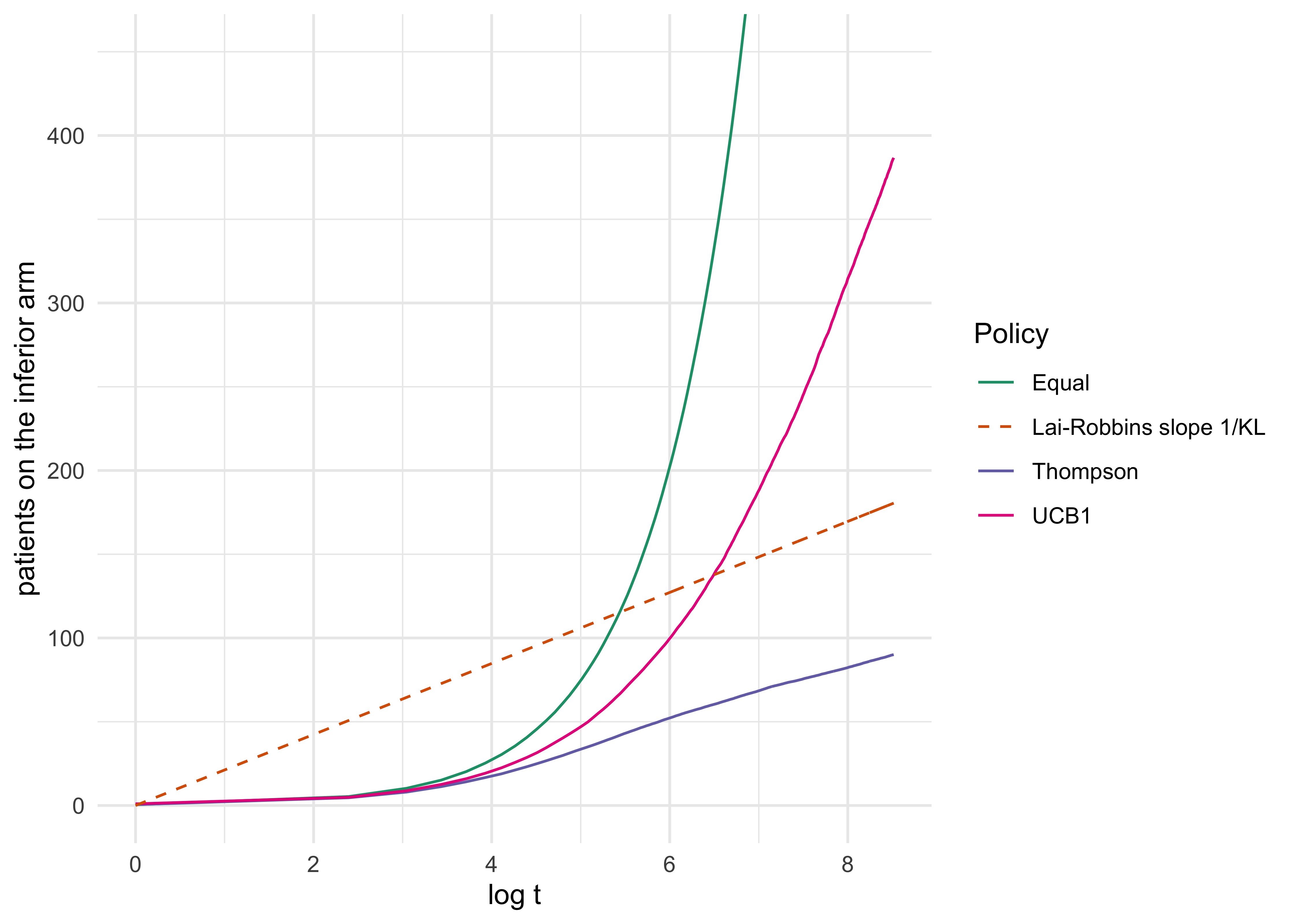
Figure 16.1 simulates the number of patients on the inferior arm for equal allocation, Thompson sampling and the UCB1 rule of Auer, Cesa-Bianchi and Fischer (Auer, Cesa-Bianchi, and Fischer 2002), which adds to each arm’s observed mean a bonus of \(\sqrt{2\log t / N_i(t)}\) and assigns the arm with the largest total.

Show the R code
pols <- c("Equal", "UCB1", "Thompson"); reg <- rar_regret_sim(pols, T = 5000, reps = 300, seed = 3)
tt <- seq(1, 5000, by = 10)
d <- data.frame(logt = log(tt), n = c(reg[tt, ]), Policy = rep(pols, each = length(tt)))
ggplot(d, aes(logt, n, colour = Policy)) + geom_line() +
  geom_line(aes(y = logt / KL, colour = "Lai-Robbins slope 1/KL"), linetype = 2) + coord_cartesian(ylim = c(0, 450)) +
  scale_colour_brewer(palette = "Dark2") + labs(x = "log t", y = "patients on the inferior arm") + theme_minimal()
Figure 16.1: Expected number of patients on the inferior arm (response 0.30 against 0.45) after t patients, 300 simulated trials per policy, plotted against log t. Equal allocation grows linearly in t, so it is exponential on this axis. Thompson sampling and UCB1 grow like log t.

At 100 patients, Thompson sampling has placed about 27 on the inferior arm against 50 for equal allocation. By 5,000 patients the figures are about 90 and 2,502, with UCB1 at about 387. These are the figures of an idealized setting: a very long horizon, an immediate binary outcome and one decision, whether to treat. A phase 3 trial is usually a few hundred patients and its outcome takes months to observe, and its main product is a statement about the drug for people outside the trial. The rest of the chapter is about what that does. The Lai-Robbins bound is asymptotic (a liminf as \(T\) grows), so finite-horizon counts can sit below the plotted slope, as Thompson sampling does at \(t = 5{,}000\) (about 90 patients against about 181 from \(\log T/\mathrm{KL}\)).

To tell an inferior arm from the best arm at error probability \(\epsilon\), a policy needs about \(\log(1/\epsilon)/\mathrm{KL}\) observations on that arm, because \(\mathrm{KL}\) is the rate at which log likelihood ratio evidence accumulates per observation. A policy that must be uniformly efficient for every possible truth cannot let the error probability on this question fall slower than polynomially in the horizon \(T\), since a mistaken commitment costs a number of patients linear in \(T\). Setting \(\epsilon \approx 1/T\) gives \(\log T/\mathrm{KL}\) observations on the inferior arm, which is Equation 16.3. The logarithm is the price of a bar that tightens with the horizon, and the argument of the next section is that the same price appears in sequential testing.

The same logarithm

Polson and Sokolov (Polson and Sokolov 2026b) observe that the scale in Equation 16.3 is the scale of the Bayes sequential boundary of Chapter 11 and the moderate deviation sample size equation of Chapter 9. We give the argument as they make it and mark which parts are exact and which are an analogy.

For contiguous alternatives (a small standardized effect \(\theta\)) the Kullback-Leibler divergence is \(\mathrm{KL} \approx \theta^2/2\). The moderate deviation relation for a test that balances the two errors is \(n\theta^2 \asymp \log n\), which in terms of divergence is \(n\,\mathrm{KL} \asymp \tfrac12 \log n\). For asymptotically optimal policies, the Lai-Robbins bound is attained in order, \(\mathbb{E}[N_i(T)]\,\mathrm{KL}_i \sim \log T\); the theorem itself supplies only the lower bound. These are the same relation with the horizon \(T\) in place of the sample size \(n\), up to a factor of two. The number of patients a bandit policy must waste on an inferior arm is the number of observations the Bayes rule needs to distinguish that arm at the moderate deviation scale.

The frequentist bandit algorithm makes the same point from the other side. UCB1 adds the bonus \(\sqrt{2\log t / N_i}\), which comes from a Hoeffding bound for rewards in \([0,1]\) whose error probability shrinks polynomially in \(t\) (as \(t^{-4}\) in the analysis of Auer and coauthors). So UCB’s confidence level also decays with the horizon, and its bonus grows like \(\sqrt{\log t}\), the same order as the Bayes bar \(\sqrt{\log T}\). The constants are not comparable in general, because the UCB radius is on the response scale and a testing boundary is on the standardized scale, so they depend on the variance proxy. Table 16.4 prints the two expressions for a unit variance proxy to show the shared growth, not a constant-by-constant comparison.

Show the R code
T <- c(1e2, 1e3, 1e4, 1e6)
kable(data.frame(Horizon = format(T, big.mark = ",", scientific = FALSE), `log T` = round(log(T), 2),
                 `UCB bar sqrt(2 log T)` = round(sqrt(2 * log(T)), 2), `Bayes bar sqrt(log T)` = round(sqrt(log(T)), 2), check.names = FALSE))
Table 16.4: The UCB exploration expression and the moderate deviation (Bayes) bar, both on a standardized scale with unit variance proxy (an illustration of shared order, not a comparison of constants). Both grow like the square root of the logarithm of the horizon, in contrast with the fixed bar z = 1.96 of a one-look level 0.025 test.
Horizon log T UCB bar sqrt(2 log T) Bayes bar sqrt(log T)
100 4.61 3.03 2.15
1,000 6.91 3.72 2.63
10,000 9.21 4.29 3.03
1,000,000 13.82 5.26 3.72

An algorithm that holds its confidence level fixed, which is the bandit analogue of an unadjusted fixed-cutoff test, has a constant probability of locking onto the inferior arm forever and suffers regret linear in the horizon. Sublinear regret needs a level that decays with the horizon. That is the lesson of Chapter 11 from a literature that was not trying to teach it: repeated marginal tests at an unchanged cutoff generally fail to control the overall error, whereas sequentially valid procedures (alpha spending, the e-process threshold \(1/\alpha\) of Chapter 12) can retain a fixed overall \(\alpha\).

Thompson sampling has no explicit bar. It draws from the posterior and plays the maximizer, so its exploration is whatever the posterior’s spread dictates, and yet Kaufmann, Korda and Munos (Kaufmann, Korda, and Munos 2012) and Agrawal and Goyal (Agrawal and Goyal 2013) showed that for Bernoulli arms it attains the Lai-Robbins bound asymptotically. The logarithm appears without being imposed. In testing the same thing happens: the Bayes factor carries an Ockham penalty of order \(\log n\) (Chapter 7) that arrives as a consequence of integrating out the parameter and not as a threshold chosen by the analyst. In both problems the Bayesian procedure gets the logarithmic scale by construction (its type I error still has to be calibrated, Chapter 14), and in both the frequentist procedure has to be told its level, as a function of the horizon, by a separate calculation. Table 16.5 sets the two problems beside each other.

Table 16.5: The two problems share a deviation scale. An unadjusted fixed cutoff fails in both; sequentially valid procedures retain a fixed overall error target.
Testing Allocation
Wrong calibration Repeated marginal tests at an unchanged cutoff \(z_\alpha\) A confidence level that does not decay with the horizon, linear regret
Pointwise tail probability for the illustrative boundary Bar \(\sqrt{\log n}\), pointwise normal-tail probability of order \((n \log n)^{-1/2}\) at each \(n\) (not the probability of ever crossing) Bar \(\sqrt{2\log t}\), regret of order \(\log T\)
Imposed by a threshold Level chosen as a function of \(n\) UCB
Supplied by the posterior The Bayes factor’s \(\log n\) penalty Thompson sampling

Russo and Van Roy (Russo and Van Roy 2016) give a third reading. They bound the regret of Thompson sampling through an information ratio, the squared expected reward shortfall divided by the information gained about which arm is best, and the bound involves the entropy of the prior over which arm is best. Regret becomes a quantity of information to be acquired divided by a rate at which it arrives, the same accounting as the Wald approximation of Chapter 11.

An analogy that does not transfer as design advice

Polson and Sokolov are explicit that the analogy is exact at the level of the deviation scale and misleading at the level of the objective, and that a recommendation of Thompson sampling for confirmatory trials on the strength of the first would be wrong. Regret is a loss in the trial. Power is a property of the final decision. Optimizing the first damages the second, and the next sections show it. As mathematics, the analogy shows that this particular normal-mixture construction shares a logarithmic scale with optimal bandit regret. As design advice it does not transfer to a trial whose conclusion will govern treatment for a population far larger than the trial. The place where it does transfer is early-phase work, where the population inheriting the decision is the next trial, and that is where the utility-based designs of Chapter 17 put it.

NoteIf it works for Amazon: Thompson sampling on the web

Hill and colleagues (Hill et al. 2017) describe how Amazon used Thompson sampling to choose among the very many layouts of a web page, searching a combinatorial space of page elements in real time. They report that after a single week of online optimization the chosen layout lifted purchases by about 21 percent over the median layout. The comparison with a trial is instructive and the transfer is limited. A click is observed in seconds, the experiment never really ends, and the visitors after the experiment matter as much as the visitors in it, so in-experiment reward is close to the right objective. A confirmatory trial has delayed outcomes, a population of future patients that may outnumber those enrolled a thousand to one, and a regulator who must trust the final estimate. That is the argument of the analogy section above and of Section 16.4.

16.3 ECMO: the case every trialist knows

What was done

Extracorporeal membrane oxygenation (ECMO) is a form of heart-lung bypass. In the early 1980s, Bartlett and colleagues were convinced that it saved newborns with persistent pulmonary hypertension and a very high predicted mortality, and that randomizing such infants to conventional medical therapy (CMT) was close to unethical. Their trial (Bartlett et al. 1985) used a randomized play-the-winner rule (Wei and Durham 1978), the randomized form of Zelen’s play-the-winner rule (Zelen 1969). In its simplest form the rule is an urn: start with one ball for each treatment, draw a ball to assign each patient, and after each outcome add a ball for the treatment that succeeded (or for the other treatment after a failure). As the urn drifted toward ECMO, one infant was assigned to CMT and died, and the other eleven were assigned to ECMO and all survived. The final tally was 11 of 11 on ECMO and 0 of 1 on CMT, with intracerebral hemorrhage in 1 of the 11 ECMO infants (Bartlett et al. 1985). A Fisher exact test of 11 of 11 against 0 of 1 gives a one-sided \(p = 1/12 = 0.083\), and Ware and Epstein (Ware and Epstein 1985) commented on the trial in the same journal.

The controversy

Ware (Ware 1989) used the trial as a case study of the difficulties of investigating therapies of potentially great benefit. The difficulty is specific. The conclusion that ECMO works rests on twelve infants, and the comparison with control rests on one death. A reader who accepts the trial does so largely because they already believe ECMO works and because the historical mortality of such infants was dreadful, and a reader who does not believe it can reasonably say that the trial did not provide the evidence. The design that was meant to reconcile ethics with science had allocated the information away from the comparison. The ethics of randomizing in such a case is treated as a problem of statistical inference by Royall (1991), who describes the randomized trial as a scientific and ethical dilemma and notes that statisticians have tended to emphasize only one side of it.

The Bayesian reading, as discussed by Kass and Greenhouse in their commentary (Kass and Greenhouse 1989) and by Berry on the ethics (Berry 1989), is more forgiving in one respect: the posterior depends on the data observed and not on the rule that produced them. With uniform priors the posteriors are \(\mathrm{Beta}(12,1)\) for ECMO and \(\mathrm{Beta}(1,2)\) for CMT, and the posterior probability that ECMO is better is \(90/91 \approx 0.989\), which the chunk below confirms by integration. With a \(\mathrm{Beta}(4,16)\) prior for CMT encoding a historical survival of about 20 percent, the probability is above 0.999. That agreement of the two priors is, of course, a statement about the data being extreme and not about the design being good.

Show the R code
f  <- function(x) dbeta(x, 12, 1) * pbeta(x, 1, 2)    # uniform priors
f2 <- function(x) dbeta(x, 12, 1) * pbeta(x, 4, 17)   # Beta(4,16) prior for CMT, 0/1 observed
kable(data.frame(Quantity = c("Uniform priors", "Exact 90/91", "Beta(4,16) prior for CMT"), `Pr(ECMO better)` = round(c(integrate(f, 0, 1)$value, 90 / 91, integrate(f2, 0, 1)$value), 4), check.names = FALSE))
Quantity Pr(ECMO better)
Uniform priors 0.989
Exact 90/91 0.989
Beta(4,16) prior for CMT 1.000

The Harvard two-stage trial

The comment on the Michigan trial was that it could not settle the question, and the Harvard group (Boston Children’s Hospital) designed a second trial with that in mind (O’Rourke et al. 1989). In the first phase infants were randomized between ECMO and CMT until a fourth death had occurred in one arm. That happened on the CMT arm: 9 of 9 ECMO infants survived against 6 of 10 on CMT. In the second phase the next 20 infants all received ECMO and 19 survived, so that overall 28 of 29 ECMO infants survived against 6 of 10 on CMT. The trial report is O’Rourke et al. (O’Rourke et al. 1989); the analysis that made it a teaching case is Ware’s (Ware 1989). The first phase alone has a one-sided Fisher \(p\) of 0.054, just short of the conventional bar, and the data from the second phase cannot be used in a randomized comparison because they were not randomized.

The UK collaborative trial

The question was settled by a conventional randomized trial in the United Kingdom (UK Collaborative ECMO Trial Group 1996). It enrolled 185 infants in 55 hospitals from 1993 to 1995 and compared referral to one of five ECMO centers with continued conventional care. It was stopped early on the advice of the data monitoring committee. Thirty of 93 infants allocated to ECMO died against 54 of 92 allocated to conventional care, a relative risk of 0.55 (95% CI 0.39 to 0.77, \(p = 0.0005\)), or about one extra survivor for every three to four infants allocated to ECMO. (Only 84% of those allocated to ECMO received it, so this is an intention-to-treat comparison of a referral policy.)

How much the prior matters

Table 16.6 collects the four data sets and two summaries computed from them: the one-sided Fisher exact \(p\) (a nominal calculation that ignores the allocation rule and the stopping design of the adaptive trials, and is omitted for the pooled Harvard rows, where the second-phase ECMO infants were not randomized) and the posterior probability that ECMO has the higher survival under independent uniform priors.

Show the R code
ed <- ecmo_data()
lab <- c(michigan = "Michigan (Bartlett 1985)", harvard1 = "Harvard, phase I", harvard12 = "Harvard, phases I and II", uk = "UK collaborative (1996)")
cmp <- lapply(ed, ecmo_beta_comparison)
kable(data.frame(Trial = lab[names(ed)],
                 ECMO = sprintf("%d/%d", sapply(ed, `[`, "yE"), sapply(ed, `[`, "nE")),
                 Control = sprintf("%d/%d", sapply(ed, `[`, "yC"), sapply(ed, `[`, "nC")),
                 `Fisher p` = ifelse(names(ed) == "harvard12", "n/a", as.character(signif(sapply(cmp, `[[`, "fisher_p"), 2))),
                 `Pr(ECMO better)` = round(sapply(cmp, `[[`, "post_prob"), 4), check.names = FALSE, row.names = NULL))
Table 16.6: The ECMO trials: survivors out of infants, the one-sided Fisher exact p (nominal: it ignores the allocation and stopping design of the adaptive trials, and is not shown for the pooled Harvard phases I and II, which combine nonrandomized ECMO infants with earlier controls), and the posterior probability that ECMO survival exceeds control survival under independent uniform priors. The Harvard rows take 28 of 29 on ECMO as given, which assumes the second phase adds only ECMO infants. The UK row counts survivors (63 of 93 and 38 of 92 are the complements of the reported deaths).
Trial ECMO Control Fisher p Pr(ECMO better)
Michigan (Bartlett 1985) 11/11 0/1 0.083 0.9890
Harvard, phase I 9/9 6/10 0.054 0.9773
Harvard, phases I and II 28/29 6/10 n/a 0.9968
UK collaborative (1996) 63/93 38/92 0.00025 0.9998

Kass and Greenhouse (Kass and Greenhouse 1989) showed in their comment on Ware’s paper how a Bayesian should handle the disagreement: not by hiding the prior but by displaying how the conclusion depends on it. Table 16.7 is our reconstruction in that spirit, not a reproduction of their priors or numbers (we did not extract those). Let \(\eta\) be the control log odds of survival and \(\theta\) the log odds ratio for ECMO. The effect prior is \(\theta \sim N(0, \sigma_\theta^2)\), centered on no effect, with \(\sigma_\theta = 0.5\) a skeptic (odds ratios beyond about 2.7 are two standard deviations out) and \(\sigma_\theta = 5\) open to almost anything. The control prior is either vague, \(\eta \sim N(0, 2^2)\), or historical, \(\eta \sim N(\mathrm{logit}\,0.4, 0.5^2)\), centered at 40 percent survival.

Show the R code
sg <- c(0.5, 1, 2, 5)
rows <- list(`Michigan, vague control prior` = ecmo_prior_sensitivity(ed$michigan, sg),
             `Harvard phase I, vague control prior` = ecmo_prior_sensitivity(ed$harvard1, sg),
             `Harvard phase I, historical control prior` = ecmo_prior_sensitivity(ed$harvard1, sg, control_prior = c(qlogis(0.4), 0.5)),
             `UK collaborative, vague control prior` = ecmo_prior_sensitivity(ed$uk, sg))
tab <- t(sapply(rows, function(r) round(r$post_prob, 3)))
colnames(tab) <- paste("SD", sg)
kable(tab)
Table 16.7: Posterior probability that ECMO is better, Pr(theta > 0 | data), by the prior SD of the log odds ratio. Our reconstruction in the spirit of Kass and Greenhouse (1989), not their numbers. Control prior vague N(0, 2^2) on the log odds of survival, or historical N(logit 0.4, 0.5^2) where stated.
SD 0.5 SD 1 SD 2 SD 5
Michigan, vague control prior 0.753 0.894 0.975 0.997
Harvard phase I, vague control prior 0.825 0.939 0.984 0.997
Harvard phase I, historical control prior 0.934 0.989 0.998 1.000
UK collaborative, vague control prior 0.999 1.000 1.000 1.000

Three things follow. To a skeptic (\(\sigma_\theta = 0.5\)) the Michigan trial is weak evidence (0.75), because almost everything it says about control survival comes from one infant. The Harvard first phase is stronger (0.83), and to anyone open to a large effect it is convincing. The historical control prior, whose information the unaugmented Fisher analysis shown here excludes, moves the skeptic to 0.93, and this is exactly where the disagreement in the 1989 discussion lives: whether that prior is well founded is the question, and the table shows how much hangs on it. By the UK trial the data swamp any of these priors (0.999 even for the skeptic), and evidence that the earlier trials only suggested was confirmed.

What the rule did to the information

The design question is cleaner than the argument about whether ECMO works. Under a randomized play-the-winner rule, how many patients end up on the control arm, and how much power does the trial have? The simulation below runs the urn with 12 infants and true survival 0.80 on ECMO and 0.20 on CMT, the extreme scenario the SIM paper uses as a stress test (Polson and Sokolov 2026a), and compares it with a fixed 6:6 trial analyzed by a one-sided Fisher exact test at level 0.025.

Show the R code
u <- rar_ecmo_urn(reps = 20000, n = 12, p = c(0.2, 0.8), m = 2000, seed = 14)

Play-the-winner puts on average about 3.7 of the 12 infants on CMT, and in about 11 percent of trials at most one, which is the situation in which a comparison is essentially impossible. Its power is 0.15, against 0.29 for a fixed 6:6 split, and neither is a trial anyone would call adequate (twelve patients is not a sample size at which any test can detect even a large effect with confidence, and the true advantage assumed here is huge). The point of the numbers is the direction. The rule gave more infants the treatment the investigators believed in, and it did so at the cost of the information the trial was meant to produce. That is the pattern of every RAR design: the benefit is in-trial reward, the price is terminal information.

The aftermath and what it means for design

A frequentist re-expression of the same logic appears in the later EOLIA trial of ECMO for adult ARDS (Combes et al. 2018), whose primary analysis gave \(p = 0.09\). A Bayesian reanalysis reported 88 to 99 percent posterior probability that ECMO reduces mortality, depending on the prior (Goligher et al. 2018). As the SIM paper puts it, this is a model-dependent re-expression of evidence, not a resolution. The SIM paper also treats the ECMO data as a prior-sensitivity stress test for a backward-induction stopping design (Chapter 15), with a \(\mathrm{Beta}(4,16)\) prior for CMT and a \(\mathrm{Beta}(1,1)\) prior for ECMO. That analysis is explicitly not a reconstruction of the play-the-winner trial and not a proposed design: it asks what a pre-specified Bayesian rule would have concluded and how fast, and it finds that with an extreme generating effect and an asymmetric historical prior the rule stops after a handful of patients per arm. Its warning is the one to carry forward. Extreme early data and an informative prior can make a rule stop almost immediately, and a protocol must show, by simulation, that this is the behavior it wants (Chapter 14).

The lessons of ECMO for RAR are three. A rule that reacts to a few early outcomes can move allocation sharply on very little evidence. The treatment that looks best early is not always best, and an urn that has drifted toward it will take a long time to correct the error. And the argument over whether the evidence was adequate is an argument about the comparison, which was thin because the design starved it.

16.4 The critiques of response-adaptive randomization

The case against, in two arms

By the 2010s the experience with Bayesian adaptive randomization in oncology produced a set of published criticisms that the practitioners of RAR now regard as the fair statement of its costs. Korn and Freidlin (Korn and Freidlin 2011) argued that in two-arm trials outcome-adaptive randomization offers little over equal allocation, while its costs in efficiency and logistics are real. Thall, Fox and Wathen (P. Thall, Fox, and Wathen 2015) collected the scientific and ethical objections, among them lower power for a given sample size, highly variable arm sizes, a non-trivial chance of putting more patients on the inferior arm than equal allocation would have, and sensitivity to time trends, and they questioned whether the ethical gain that motivates RAR survives these defects. Hey and Kimmelman (2015) argue that the ethical advantage claimed for outcome-adaptive allocation does not survive scrutiny in two-armed or early-phase studies. The summaries here follow the papers’ main arguments and are not exhaustive. Wathen and Thall (Wathen and Thall 2017) followed with a simulation study of multi-arm trials, and Proschan and Evans (Proschan and Evans 2020) titled their review as advice: resist the temptation. The balanced review of Robertson and coauthors (Robertson et al. 2023) separates the myths from the practical considerations and arrives at guidance that this chapter follows: use a burn-in, restrict extreme allocation, model time trends, and justify the ethical claim explicitly.

The case for, and the replies

The critiques have replies, and a fair account gives them. Berry and Eick (1995) analyzed adaptive assignment against balanced randomization as a decision problem whose objective is to treat as many patients, in and out of the trial, as effectively as possible. Randomization is satisfactory when the disease is at least moderately common, and adaptive procedures can play a role when a substantial proportion of all patients with the disease are in the trial. That is the premise the later simulations test, and, on our reading, the two-arm trials of the critique are mostly settings with a large population outside the trial. Villar, Robertson, and Rosenberger (2020) is a reply to the review of Proschan and Evans, and Villar, Bowden, and Wason (2018) propose response-adaptive designs for binary responses that keep patient benefit while being robust to time trends. Lee, Chen, and Yin (2012) revisited the usefulness of outcome-adaptive randomization, and Wason and Trippa (2014) compared Bayesian adaptive randomization with multi-stage designs for multi-arm trials, which puts the cost of RAR against alternatives that also drop arms early. On our reading the case is weakest in a two-arm confirmatory trial with a large outside population, and strongest with several arms and a small population (Section 16.6), provided the ethical claim is made explicitly and the design guards against drift (Section 16.5). This is not a point of agreement: P. Thall, Fox, and Wathen (2015) and Wathen and Thall (2017) argue that the problems persist with several arms.

Reproducing the critique

We simulate the two-arm trial of the Polson and Sokolov example: 400 patients, response 0.30 on control and 0.45 on the experimental arm, binary outcome observed immediately, outcomes analyzed by a one-sided pooled \(z\) test of two proportions at \(\alpha = 0.025\). Three allocation rules are compared. Equal 1:1 is the traditional design, here simple randomization with probability one half (permuted blocks would give exact balance within periods). Thompson uses the posterior probability that the experimental arm is better, recomputed after every batch of 20 patients. Capped Thompson adds a burn-in of the first 25 percent of patients at 1:1 and then bounds the allocation probability between 0.10 and 0.90 (the bounds are enforced exactly, with the probabilities still summing to one). The simulator is rar_simulate() in the package, wrapped by rar_two_arm(). We report the number of responders in the trial, the share of patients on the better arm, the number of patients on the inferior arm, the standard deviation of the number of patients on the better arm (how variable the design is from trial to trial), and power.

Show the R code
two <- rar_two_arm(reps = 5000)
kable(with(two, data.frame(Rule = rule_name, Responders = round(resp, 1), `Share on better arm` = pct(share_best), `Patients on inferior arm` = round(n_inferior),
  `SD of n on better arm` = round(sd_n_best), `Trials with fewer than half on the better arm` = pct(frac_more_on_inferior, 1), Power = pct(rej_best_naive, 1), `Power, stratified` = pct(rej_best_strat, 1), check.names = FALSE)))
Table 16.8: Two-arm binary trial, n = 400, response 0.30 (control) and 0.45 (experimental), 5,000 simulated trials per rule, no drift. Power is one-sided at level 0.025; the last column is the power of the analysis stratified by enrollment period (Section 16.5).
Rule Responders Share on better arm Patients on inferior arm SD of n on better arm Trials with fewer than half on the better arm Power Power, stratified
Equal 1:1 150.0 50% 200 10 47.1% 87.6% 87.3%
Thompson 172.3 87% 53 41 1.2% 61.1% 49.0%
Capped Thompson 166.6 78% 89 22 0.7% 73.2% 64.0%

The results confirm the critique and the original Polson and Sokolov table to within simulation error. Thompson sampling puts about 87% of patients on the better arm and adds about 22 responders to the trial, but power falls from 88% to 61%. The number of patients on the better arm has a standard deviation of about 41 from trial to trial, against 10 for equal allocation, which is the variability Thall and colleagues describe. The critique that RAR often puts more patients on the inferior arm than equal allocation would is weaker here. Fewer than half of the patients end up on the better arm in about 1% of Thompson trials (the equal-allocation figure of 47% is only sampling noise around a count centered at 200). In this scenario the effect is large, the outcome is immediate and the posterior converges quickly, and the costs that remain are power and variability.

Capped Thompson recovers part of the power (73%) and keeps 78% of patients on the better arm, at a cost of about 6 responders relative to uncapped. In both cases, the trade is what Polson and Sokolov describe: for a 400-patient trial whose conclusion will govern treatment of many more patients, the loss of 14 to 26 points of power is not a trade a sponsor should accept in a confirmatory setting.

For a binary outcome the variance of the estimated difference is approximately \(p_1(1-p_1)/n_1 + p_0(1-p_0)/n_0\), where \(n_1\) and \(n_0\) are the realized arm sizes. When allocation is driven by the data, \(n_0\) falls quickly once arm 1 looks better and the term \(p_0(1-p_0)/n_0\) dominates, so the standard error is much larger than that of the 1:1 design at the same total \(n\). With 87 percent of 400 patients on the better arm, \(n_0 \approx 52\) and the standard error is about 1.4 times the 1:1 value. In addition \(n_0\) is random and correlated with the outcomes, which is why the nominal \(z\) test is no longer exactly standard normal under the null: the simulation below finds a type I error of about 0.049 for Thompson sampling, almost twice the nominal 0.025, even with no drift.

16.5 Time trends: the failure that matters most

The mechanism

RAR reacts to accumulating data, which means it reacts to chance. Under the null hypothesis, if the experimental arm happens to look better in the early patients, RAR sends it more of the later patients. Outcome-adaptive allocation can invalidate the naive analysis even without drift (the no-drift Thompson analysis above has type I error near 0.049 against a nominal 0.025). Changes in the patient population add confounding with calendar time. Suppose the background response rate rises during enrollment, because the standard of care improves, the site mix changes, a referral pattern shifts, or a variant changes. The arm that benefited from early luck now receives more of the later, healthier patients, and it looks better still. The bias runs through allocation alone. Nothing about the treatment has changed, and the comparison of response rates is confounded with calendar time.

This is the central practical objection to RAR in confirmatory trials, and it is the property that fixed allocation with permuted blocks was designed to defeat. The FDA draft on master protocols and the EMA draft both refer to the same mechanism: changes in the allocation probability over time introduce time-varying selection bias, so comparisons should use concurrent controls and the analysis can be hard to adjust.

Simulation

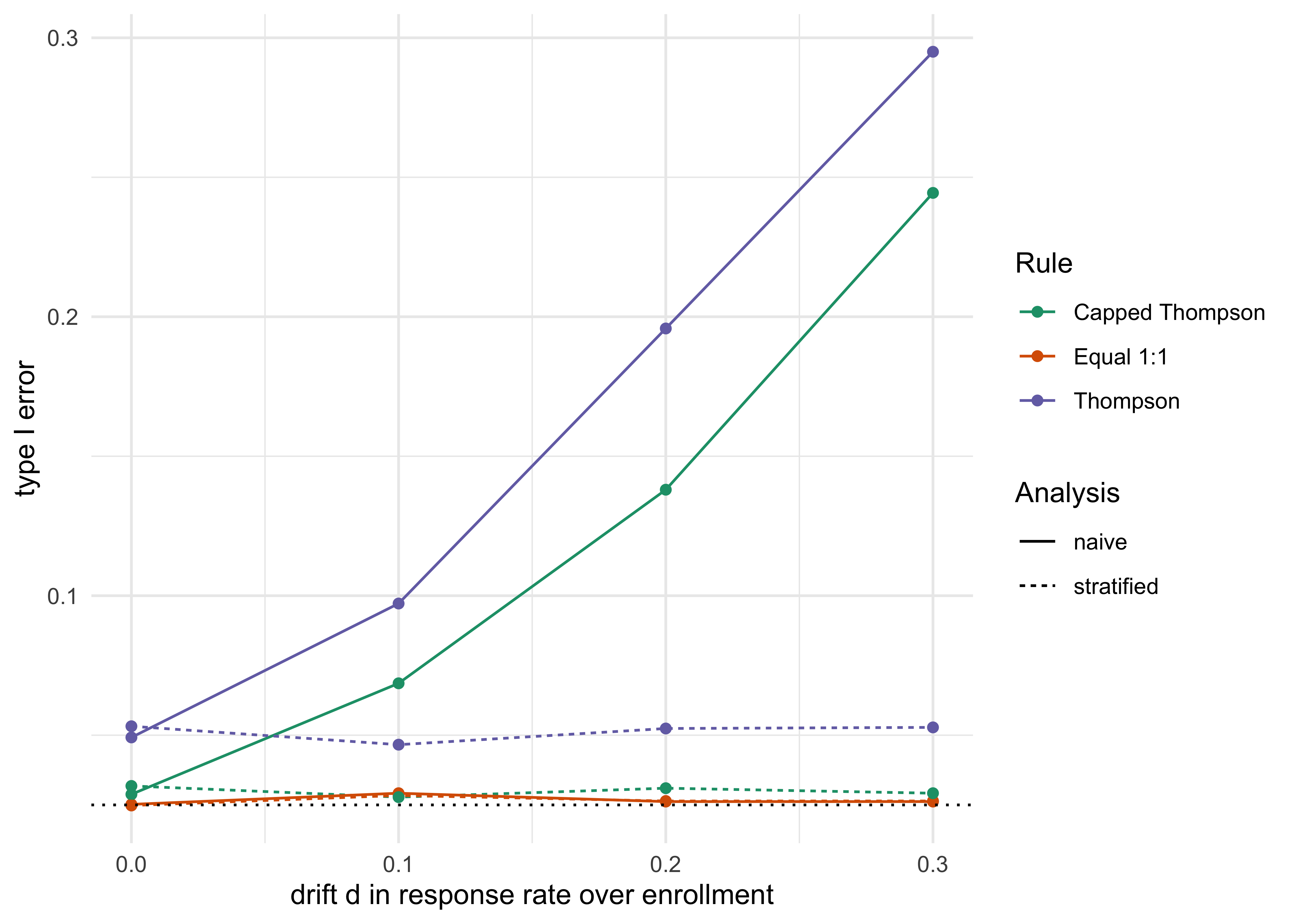
We simulate a null trial (response 0.30 in both arms) in which the response probability of every patient rises linearly from \(0.30 - d/2\) at the first patient to \(0.30 + d/2\) at the last, with drift \(d\) from 0 to 0.30. In the larger values this is a very large change in the patient mix across enrollment; the range is chosen to show the shape of the effect and not to describe a typical trial. Two analyses are applied to each trial. The naive analysis is the pooled \(z\) test. The stratified analysis divides enrollment into four consecutive periods, forms the difference in response rates within each period, and combines them with Mantel-Haenszel-type weights. Type I error is the probability that the experimental arm is declared better at one-sided level 0.025.

Show the R code
sweep <- rar_drift_sweep(reps = 5000)
d <- rbind(data.frame(sweep[c("rule_name", "drift")], err = sweep$rej_any_naive, Analysis = "naive"),
           data.frame(sweep[c("rule_name", "drift")], err = sweep$rej_any_strat, Analysis = "stratified"))
ggplot(d, aes(drift, err, colour = rule_name, linetype = Analysis)) + geom_line() + geom_point() + geom_hline(yintercept = 0.025, linetype = 3) +
  scale_colour_brewer(palette = "Dark2", name = "Rule") + labs(x = "drift d in response rate over enrollment", y = "type I error") + theme_minimal()
Figure 16.2: Type I error (one-sided, nominal 0.025) of the experimental-versus-control comparison under the null, as the response rate drifts upward by d over the course of enrollment. Solid lines: naive pooled analysis. Dashed lines: analysis stratified by enrollment period. 5,000 simulated trials per point, n = 400.
Show the R code
w <- function(d, k) round(sweep[[k]][sweep$drift == d], 3)
kable(data.frame(Rule = unique(sweep$rule_name), `d = 0 naive` = w(0, "rej_any_naive"), `d = 0 stratified` = w(0, "rej_any_strat"),
                 `d = 0.2 naive` = w(0.2, "rej_any_naive"), `d = 0.2 stratified` = w(0.2, "rej_any_strat"), check.names = FALSE))
Table 16.9: Type I error under the null (0.30 versus 0.30), n = 400, for drift d = 0 and d = 0.20. Nominal level 0.025 one-sided.
Rule d = 0 naive d = 0 stratified d = 0.2 naive d = 0.2 stratified
Equal 1:1 0.025 0.025 0.026 0.026
Thompson 0.049 0.053 0.196 0.052
Capped Thompson 0.029 0.032 0.138 0.031

The pattern is clear. Under equal allocation, drift is harmless: the type I error stays at its nominal level even for a 30-point drift, because allocation does not depend on the outcomes, so each period contributes equally to both arms in expectation. Under Thompson sampling, the naive test has a type I error that climbs with the drift, from 0.049 with none to 0.196 at \(d = 0.2\) and 0.295 at \(d = 0.3\), many times the nominal level. Capped Thompson reduces the problem (0.029 with no drift, 0.138 at \(d = 0.2\)) but does not remove it. A trial that drifts by 20 points has roughly a one-in-seven chance of declaring a useless drug effective under capped Thompson, and roughly one in five under plain Thompson.

The fixes

Three fixes are standard, and they should be pre-specified as a package.

Stratify the analysis by enrollment period. If allocation probabilities are fixed within each period and the analysis compares arms only within a period, then the allocation within a period is independent of the outcomes in that period and each stratum is a valid comparison. The type I error stops growing with the drift, as the dashed lines show: 0.047 to 0.053 for Thompson (about twice nominal), 0.028 to 0.032 for capped Thompson. The remaining excess for plain Thompson (about 0.05, not 0.025) comes from allocation updating within a period and from small-count behavior of the \(z\) test, and is removed by calibrating the critical value by simulation (Chapter 14). The price is power. In the no-drift table of the previous section, the stratified analysis has power 49% under Thompson and 64% under capped Thompson (the corresponding naive figures are 61% and 73%), because comparing within periods discards the information in between-period contrasts when allocation is unbalanced across them. Pre-specified adjustment for calendar time as a covariate in a regression model is the continuous counterpart, with the same trade.

Burn-in and a cap. Start with a period of fixed 1:1 allocation, and keep the allocation probability away from 0 and 1. A burn-in prevents the first handful of outcomes from steering the whole trial, as the urn in ECMO did. A cap guarantees that every arm keeps contributing concurrent data, which is what makes later calendar-time adjustment possible. The cap reduced the type I error from 0.196 to 0.138 at \(d = 0.2\) in the table above, which is helpful but not sufficient alone.

Keep the control allocation fixed. Hold the control arm at a pre-specified share, and let only the experimental arms trade patients. The comparison of each experimental arm with the control then rests on a control stream that is balanced in time. This keeps the control stream balanced in time and is the fix with the best operating characteristics in the multi-arm simulation below. It does not by itself make the design acceptable to regulators: the FDA master protocols draft describes a larger fixed control allocation as appropriate, but the ratio of each experimental arm to control still changes with the data, and the EMA draft recommends fixed ratios for every comparison of interest. In a two-arm trial there is nothing left to adapt once the control is fixed, which is the honest reason that two-arm RAR is hard to defend.

A fourth route is to model the time trend instead of designing around it. The platform-trial literature smooths the control rate across calendar periods and borrows from non-concurrent controls with discounting, the Bayesian time machine of Saville et al. (2022), which is developed in Chapter 20. For multi-arm binary trials, Villar, Bowden, and Wason (2018) studied protected control allocation and found approximately nominal error under the time trends examined. They also assessed randomization-based inference and regression adjustment. The protocol should prespecify the allocation rule and analysis method, and simulations should assess plausible drift and any time-model misspecification.

TipIn the protocol: pre-specifying a response-adaptive randomization rule

If a protocol includes RAR, the statistical analysis plan should state, before the first patient is enrolled:

  • the allocation rule in full (for Thompson-type rules, the formula, the tuning exponent if any, and the update frequency);
  • the burn-in size and the lower and upper bound on each arm’s allocation probability;
  • the share of patients on the control arm and whether it is fixed;
  • the primary analysis, including how enrollment period or calendar time enters it, and the estimand (ICH E9(R1));
  • the simulation report: type I error under the null and under pre-specified drift scenarios (a monotone drift of at least 10 and up to 20 percentage points in the control response is a reasonable starting range), power, expected patients per arm, and the distribution of the allocation, not only its mean;
  • how the allocation algorithm is shielded: who runs it, who sees the allocation probabilities, and how the sponsor’s blinding is preserved (the DMC charter of Chapter 23).

16.6 When response-adaptive randomization helps: many arms

The multi-arm case

The strongest argument for RAR is not the two-arm trial but the trial with several experimental arms (doses, regimens, or drugs) and a shared control. Two things differ. First, there are many inferior arms, so equal allocation wastes a larger share of the trial (75 percent of patients are on arms other than the best one in a four-arm trial with one best). Second, the comparison that matters, best arm against control, can be protected by fixing the control share while the experimental arms compete for the rest. This is the setting of I-SPY 2 (Barker et al. 2009) and REMAP-CAP (Angus et al. 2020) (both in Section 16.9 below, with BATTLE) and the one in which the review of Robertson and coauthors (Robertson et al. 2023) finds the best case for RAR. Wathen and Thall (Wathen and Thall 2017) study the multi-arm setting by simulation.

We simulate a four-arm trial: a control at 0.30 and three experimental arms at 0.30, 0.40 and 0.50, 600 patients, with the same batch size of 20. The four rules are equal allocation, Thompson sampling with allocation proportional to the posterior probability that each arm is best (the multi-arm form of Thompson’s rule, which generalizes to arbitrary exponents as in Thall and Wathen (P. F. Thall and Wathen 2007)), capped Thompson with a burn-in and a floor of 2.5 percent on each arm, and the same capped rule with the control share held fixed at 1/4 and the remaining three quarters divided among the three experimental arms by their posterior probabilities of being best among the experimental arms (control excluded). Power is for the best arm (0.50) against control, with a Bonferroni level of \(0.025/3\) for each experimental arm. Power and type I error are reported for the same prespecified analysis, first the naive pooled test and then the period-stratified one. Bonferroni gives familywise control only when each component test is valid, and the naive test is not valid under drift, so no claim of strong familywise control is made here: that would need calibration across nuisance values and partial-null configurations.

Show the R code
fa <- rar_four_arm(reps = 3000)
kable(data.frame(Rule = fa$alt$rule_name, Responders = round(fa$alt$resp), `Patients not on best arm` = round(fa$alt$n_inferior),
  `Share on control` = pct(fa$alt$share_ctrl), `Power, naive` = pct(fa$alt$rej_best_naive, 1), `Power, stratified` = pct(fa$alt$rej_best_strat, 1),
  `Type I, naive, d=0.2` = pct(fa$null$rej_any_naive, 1), `Type I, stratified, d=0.2` = pct(fa$null$rej_any_strat, 1), check.names = FALSE))
Table 16.10: Four-arm trial (control 0.30, experimental 0.30, 0.40, 0.50), n = 600, 3,000 simulated trials per rule. Power is for the best arm against control, one-sided, Bonferroni level 0.025/3, for the naive and the period-stratified analyses. The last two columns are the type I error (probability of declaring any experimental arm better) of the same two analyses under the global null with a drift of 0.20 in the response rate over enrollment.
Rule Responders Patients not on best arm Share on control Power, naive Power, stratified Type I, naive, d=0.2 Type I, stratified, d=0.2
Equal 225 450 25% 87.2% 87.2% 1.6% 1.5%
Thompson 276 164 6% 49.5% 34.8% 16.9% 1.0%
Capped Thompson 267 215 9% 68.1% 49.7% 13.2% 1.7%
Capped, control fixed at 1/4 250 298 25% 93.3% 92.9% 3.4% 1.4%

The first three rows repeat the two-arm lesson with more force. Uncapped Thompson sampling puts 73% of patients on the best arm and adds about 51 responders to the 225 of equal allocation, but because it also reduces the control group to about 6% of the trial, power for the comparison with control falls from 87% to about 50%, and a drifting response rate pushes the familywise type I error of the naive analysis to 17%. Capping helps (power 68%) but is not sufficient (type I error 13% under drift).

The fourth row is the result that justifies RAR. With the control fixed at one quarter of the trial, a burn-in and a floor, the design places about half of the 600 patients on the best arm (against a quarter under equal allocation), delivers about 24 more responders than equal allocation, and has higher power than equal allocation for the best arm versus control (93% against 87% for the period-stratified analysis, 93% against 87% for the naive one), because the best arm now has about 300 patients to compare with the control’s 150. The two analyses must be read each against its own error. For the stratified analysis the type I error under a 20-point drift is 1.4%, against 1.5% for equal allocation, so the power of the stratified analysis (93%) is the one to quote. For the naive analysis it is 3.4%, above the 2.5 percent target by about three Monte Carlo standard errors (0.3 points at 3,000 trials), so the naive power is not a power one can claim. Both error rates are under the global null only; partial nulls and other nuisance values would have to be checked before the procedure is called error-controlled. The gain is the observation that in a multi-arm trial much of the sample would be spent on arms that are visibly not going to win, and a design that moves that sample to the contender, while the control comparison stays balanced in time, spends it on the question being asked.

Two caveats keep the result honest. The power reported is for the best arm. The 0.40 arm gets less data under the adaptive rule than under equal allocation and its comparison with control has lower power, so if the question is to estimate every dose, equal allocation is the better design. And the result depends on the effect being large enough, and the endpoint fast enough, for the allocation to converge in the trial. With a delayed endpoint, the allocation moves on information that is months old, and the gain shrinks. A simulation that mimics the real lag between enrollment and outcome is a required part of the design report.

Dunnett-type and fixed control allocation

The fixed control share in the fourth row is 1/4, the share equal allocation would give. The Dunnett sqrt(k) share for three experimental arms is 36.6 percent (Table 16.2). A protocol that wants the best control comparison in a fixed design should use the latter, and a protocol with RAR among the experimental arms can choose any fixed share it can defend. The regulatory text asks for the choice to be justified and the ratio to be held fixed, and says nothing that requires either number. The extra control patients increase the power for every comparison with control and cost experimental-arm allocation, a trade the simulation report should show.

Where RAR fits

The conditions under which a case for RAR can be made are those the simulations suggest and the literature endorses (Robertson et al. 2023). There are several experimental arms, so there is a lot to be saved from visibly inferior arms. The primary endpoint is observed quickly relative to the enrollment period, so allocation has something to learn from. The trial is large enough for the allocation to converge, and small enough in population that the in-trial benefit matters (a rare serious disease, an early-phase screening trial). The control share is fixed and concurrent controls are used. And the trial’s regulatory role is exploratory or seamless-with-confirmation, not the single confirmatory comparison of record. The platform designs of Chapter 20 and the dose-finding designs of Chapter 17 are where these conditions are most often met. Where they are not (two arms, a slow endpoint, a confirmatory objective) the traditional design wins, and a sponsor that chooses RAR anyway owes the regulator a simulation that shows what it buys.

16.7 What the regulators say

The regulatory texts agree on the principle and differ on strictness. The principle is that RAR is an adaptive design feature and so falls under the general requirements for adaptive designs: prospective planning, control of the false positive rate, reliable estimation, and integrity of the trial. The differences are in how much the text expects a sponsor to justify it.

FDA, Adaptive Designs (2019). Changes to allocation fall within its definition of an adaptive design (anchor above; Chapter 3). The drift simulation above illustrates its warning that adaptive features can inflate the type I error probability, and it expects the analysis, not only the allocation, to be pre-specified, since an analysis that ignores how patients were assigned can be biased. It does not forbid RAR. It places the burden of proof on the sponsor.

ICH E20 (draft, June 2025). For RAR in confirmatory trials the “clear and compelling justification” is the argument of Section 16.6: why the adaptive design is better than a fixed one for this question, shown by simulation under realistic drift and delay. For a two-arm confirmatory trial, Table 16.8 and Table 16.9 are what a reviewer would produce to ask for the justification.

FDA Bayesian draft (January 2026). Nothing in the Bayesian label relaxes the above. This chapter takes calibration by simulation as the default (anchor above). A Bayesian design with RAR is a design with a Bayesian analysis and a data-dependent allocation, and the calibration by simulation (Chapter 14) must include the allocation rule and the drift scenarios. A Bayesian analysis does not by itself solve the confounding of calendar time with arm in a drifting trial. The posterior is conditional on the data, which is why a Bayesian can say that the stopping rule is ignorable, but the model for those data must contain the drift for the posterior to be right.

FDA master protocols (revised draft, June 2026). Its worked examples of ratio changes are fixed schemes in which the ratio changes as drugs enter or leave a platform, not changes driven by outcome data, so it does not address outcome-driven allocation there. It asks that the primary analysis use only concurrently eligible controls.

EMA, draft reflection paper on confirmatory platform trials (October 2026). The EMA text is the strictest: it reasons that changes in allocation probability over time can cause time-varying bias that is difficult to adjust for, and concludes that response-adaptive randomization is not supported in confirmatory platform trials. It is a draft. A sponsor with a global program should assume that RAR in the confirmatory trial of record will be queried in Europe. The draft’s conclusion concerns confirmatory platform trials; exploratory and seamless-stage uses still need case-specific justification and agency discussion.

Table 16.11: Fixed allocation and response-adaptive randomization, side by side.
Traditional fixed allocation Bayesian RAR
Allocation Fixed ratio, usually 1:1, by blocks Probability updated from accumulating outcomes
Basis in regulation Default of ICH E9, 21 CFR 314.126 Adaptive design under FDA 2019 and E20 draft, with justification
Type I error Exact from the design (randomization or normal theory) By simulation, including drift and delay scenarios
Time trends Balanced by blocks Must be handled by stratified or model-based analysis
Power for a fixed n Highest in the two-arm case Lower in two-arm trials, can be higher in multi-arm trials with fixed control
Patients on inferior arms Equal share Fewer, with higher variability
Where regulators are comfortable Confirmatory trials Exploratory, multi-arm, early phase; a fixed control share alone does not establish acceptability, and the EMA draft does not support RAR in confirmatory platform trials

What stays the same is the objective: a comparison that meets the standard of substantial evidence (Chapter 3). What changes is where the burden lies. Some designs, conventional or adaptive, permit analytic or exact recursive evaluation of their operating characteristics; designs with data-driven allocation generally require simulation. Both conventional and Bayesian designs require justification of the complete procedure, including the analysis, the multiplicity handling, the estimation and the operations. For the adaptive trial of this chapter the operating characteristics are known from the simulation report, so the sponsor must make the case, scenario by scenario.

16.8 Practical guidance

For a confirmatory two-arm trial, use fixed allocation. The simulations of this chapter and the critiques of Korn and Freidlin and of Thall and colleagues point the same way: at best a small gain to in-trial patients, a loss of power, and a new route to type I error inflation. If ethics requires protecting patients inside the trial, use a group sequential design with a futility and efficacy boundary (Chapter 11 and Chapter 15), which achieves much of the saving without touching allocation. SHINE (Section 16.9) paired a group sequential design with limited adaptive allocation.

For a multi-arm trial or a platform, decide whether to adapt among experimental arms, and if so, fix the control share, include a burn-in, cap the allocation probabilities, analyze with concurrent controls, adjust for calendar time, and report type I error under drift, together with the power for each experimental arm and not only the best. Chapter 20 develops the platform setting, including how arms enter and leave. Chapter 17 develops the early-phase use, where Thall’s utility-based designs are the strongest case for RAR because the objective there is to choose a dose for the next trial.

For a rare disease, where equal allocation means half of a handful of patients on an arm that may be inferior, a Bayesian design with RAR can be the least bad option and may be the only one the community will accept. The same safeguards apply, and so does the warning from ECMO: the more extreme the allocation, the less information the trial produces about the comparison that regulators will have to judge.

16.9 In practice: four trials

The trials below use adaptive allocation, or sit next to it, in settings where the chapter’s conditions are partly met. The facts are from the primary reports cited in each subsection.

I-SPY 2

I-SPY 2 is a neoadjuvant breast cancer platform with ten prospectively defined biomarker signatures (all patients, HR+, HR-, HER2+, HER2-, MammaPrint high-2, and the four HER2 by HR combinations). Patients are classified into eight mutually exclusive subtypes defined by HR, HER2 and MammaPrint status for adaptive randomization, and efficacy and graduation are assessed in the ten overlapping signatures. The allocation probability of each experimental arm follows its current Bayesian probability of success in the subtype, so arms that look better receive more patients, while a fixed share of patients goes to control (Park et al. 2016; Nanda et al. 2020). No experimental arm exceeds 120 patients, and the model is a covariate-adjusted logistic regression on pathologic complete response (pCR) (Park et al. 2016). The graduation and futility rules, which are written in predictive probability, and the neratinib and pembrolizumab results are in Section 15.10. The lesson for this chapter is the multi-arm one of Section 16.6. Adaptation among experimental arms, with a concurrent control, serves a screening purpose, and the platform pays for it with a conservative graduation bar and a later confirmatory trial.

REMAP-CAP

REMAP-CAP (Angus et al. 2020) is a platform in which several domains of treatment are randomized at once, and its protocol allows response-adaptive updating of allocation within a domain. What is documented are the Bayesian stopping triggers in the interleukin-6 receptor antagonist domain (REMAP-CAP Investigators et al. 2021): efficacy if the posterior probability of an odds ratio above 1 against control exceeds 99 percent, futility if the probability of an odds ratio above 1.2 is below 5 percent, with neutral priors and a hierarchical model that nests tocilizumab and sarilumab under an overall IL-6 effect. At the interim analysis of 28 October 2020, tocilizumab met the efficacy criterion (posterior probability 99.75 percent, odds ratio 1.87, 95 percent credible interval 1.20 to 2.76), and assignment to control closed on 19 November. The final adjusted odds ratio on organ-support-free days was 1.64 (1.25 to 2.14) for tocilizumab. Here the adaptation is in the stopping rule, a posterior probability, and the report was made while the platform kept running. The lesson is the one the drift simulation teaches: the analysis adjusts for 2-week time epochs, site and age, which is the calendar-time adjustment that adaptive allocation requires.

BATTLE

BATTLE (Kim et al. 2011; the design is in Zhou et al. 2008) was a biopsy-mandated trial of pretreated advanced non-small cell lung cancer with about 255 patients and four treatments (erlotinib, vandetanib, erlotinib plus bexarotene, sorafenib). After an initial period of equal randomization, a Bayesian probit model moved allocation toward the treatments performing better within biomarker groups. It is described as the first completed biomarker-based, adaptively randomized trial in this disease. An earlier Bayesian adaptive randomization design for recurrent glioblastoma, evaluated retrospectively on four phase 2 trials, is Trippa et al. (2012). The lesson is the caution of Section 16.6 and Section 16.5: allocation among treatments inside small biomarker strata moves on little data, so the burn-in, the cap and an analysis that respects calendar time matter more, not less.

SHINE and its Bayesian re-analysis

SHINE (NCT01369069) compared intensive with standard glucose control for 72 hours in acute ischemic stroke with hyperglycemia. Its design combined group sequential stopping with response-adaptive randomization, and it was not a Bayesian trial. It found no significant difference in favorable 90-day outcome, and severe hypoglycemia occurred in 15 of 581 patients (2.6 percent) on intensive treatment (Johnston et al. 2019). A later paper compared the Bayesian adaptive design developed in the ADAPT-IT project with the frequentist design that was used, in a retrospective comparison (Broglio et al. 2022). The lesson is regulatory in tone: a confirmatory-scale trial can combine a classical error-controlled stopping rule with limited adaptation of allocation, which is the conservative end of what Section 16.7 describes, and a Bayesian alternative is judged against it by simulation and not by assertion.

TipTry it in the lab

Open Module 9, https://nytel.ai/testing/09-adaptive-bayesian.html, and go to “Send more patients to the winner” (control 30 percent, new drug 50 percent). Before running a trial, predict how many more successes Thompson sampling will give than the 80 expected from an equal split of 200 patients, then run ten more trials and check. Then open the Studio, https://nytel.ai/testing/14-studio.html, switch the allocation from fixed to adaptive and add a drifting scenario: read the operating-characteristics table for power and type I error. The lab shows the gain in successes, and the book and the Studio show the price.

Key points

  • Fixed 1:1 allocation is the default because it maximizes power for a given total, makes the randomization distribution exact, and balances calendar time within blocks. Unequal fixed ratios cost 12.5 percent more patients at 2:1 and a third more at 3:1.
  • Allocation is a bandit problem. Thompson sampling assigns each patient to an arm with probability equal to its posterior probability of being best. The Gittins index solves the discounted infinite-horizon problem exactly, and the Lai-Robbins bound says the best possible regret grows like \(\log T\).
  • The logarithm that governs bandit regret is the same logarithm that governs the Bayes sequential boundary: \(n\,\mathrm{KL} \asymp \tfrac12\log n\) against \(\mathbb{E}[N_i]\,\mathrm{KL}_i \sim \log T\) for asymptotically optimal policies (Polson and Sokolov). Repeated marginal tests at an unchanged cutoff fail in both. The analogy is exact for the scale and does not transfer as design advice, because regret is a loss in the trial and confirmatory power is a property of the final decision.
  • In a two-arm trial of 400 patients (0.30 against 0.45), Thompson sampling adds about 22 responders and cuts power from about 88% to about 61%, with much larger variation in the arm sizes.
  • Drift in the response rate over enrollment breaks RAR. With a 20-point drift the type I error of the naive test is about 0.196 under Thompson sampling and 0.138 under capped Thompson against 0.025 nominal, and it is unaffected under equal allocation. Stratifying the analysis by enrollment period removes the effect of drift (capped Thompson about 0.031; plain Thompson stays near 0.05 until the critical value is calibrated by simulation), at a cost in power.
  • In a multi-arm trial with a fixed control share, a burn-in and a cap, RAR gave about 24 more responders, about half of the patients on the best arm, and higher power for the best arm than equal allocation, reported for the period-stratified analysis (93% against 87%) with its type I error under drift (1.4%); the naive analysis of the same design has type I error 3.4% and its power is not claimable.
  • ECMO illustrates the cost of aggressive allocation: play-the-winner moved nearly all infants to one arm and starved the comparison that the trial existed to make.
  • Regulators accept RAR as an adaptive feature subject to FDA 2019 and E20 (clear and compelling justification, limited adaptations), expect simulation including time trends, and describe a larger fixed control share as appropriate (which protects control accrual but does not by itself establish acceptability of adaptive allocation among experimental arms). The EMA draft of October 2026 recommends fixed allocation ratios and concludes that response-adaptive randomization is not supported in confirmatory platform trials.
NoteDiscussion questions
  1. A sponsor proposes 2:1 allocation to the experimental arm in a two-arm confirmatory trial because “patients prefer it”. What does the 2:1 design cost in sample size for the same power, and is that cost the same as the cost of a data-driven shift to 2:1 halfway through enrollment? Which of the two does the FDA 2019 guidance treat as an adaptive design?
  2. In the drift simulation, equal allocation has the right type I error at any drift and Thompson sampling does not. Explain in words why blocking in calendar time protects the first and why data-dependent allocation exposes the second. What would you add to the SAP to defend a Thompson design against this objection?
  3. In the four-arm simulation, the adaptive design with a fixed control has higher power for the best arm than equal allocation, while in the two-arm simulation every adaptive rule has lower power. What is different? For which arm of the four-arm trial does the adaptive design have lower power than equal allocation, and does that matter for the objective of the trial?
  4. Polson and Sokolov say the bandit analogy is “exact at the level of the deviation scale and misleading at the level of the objective”. Restate this for a clinician. Where in the development program (phase 1b, phase 2, phase 3, platform) is the in-trial reward the right objective?
  5. The Bartlett ECMO trial put 11 infants on ECMO and 1 on conventional therapy. Posterior probabilities were over 0.98 under both priors we tried. Should the regulator have accepted it as substantial evidence? What does the answer depend on besides the posterior probability?