A group sequential design is a promise made in advance. The protocol states how many looks there will be, at what information fractions, and which boundary applies at each; the type I error is then controlled because the analyst did exactly what the protocol said. Most of the time that is how a trial is run, and Chapter 11 showed that the machinery behind it is sound. But anyone who has sat on a data monitoring committee knows the promise is sometimes hard to keep. A competing trial reports early and the committee wants an extra look. A safety signal prompts an unscheduled unblinded review. The sponsor asks whether enrollment can be extended by 200 patients because the interim estimate is promising but the boundary was not crossed. Each of these is a look the protocol did not plan. For a classical fixed boundary schedule an unplanned look is outside the guarantee, although a spending-function design can accommodate a look whose timing does not depend on the accumulating comparative results.
This chapter introduces a family of methods whose guarantee does not depend on the schedule. They are called anytime-valid, and the central object is the e-value: a nonnegative number that can be read as the outcome of a fair bet against the null hypothesis, and that can be updated as data arrive. The idea has a long history (Ville 1939 (Ville 1939), Wald’s sequential probability ratio test (Wald 1945), Robbins’s work on boundaries that hold for every sample size (Robbins 1970)) and a recent revival (Shafer and Vovk 2019; Shafer 2021; Vovk and Wang 2021). We follow the treatment of Sokolova and Sokolov (A. O. Sokolova and Sokolov 2026) and the working papers of Polson and Sokolov (Polson and Sokolov 2026c, 2026b).
The chapter has a second purpose. The guarantee has a price in the construction studied here, and the price can be stated in one line: for the normal-mixture e-value, at large information the anytime-valid rule needs approximately \(2\log(1/\alpha)\) more units of squared evidence than a Bayesian rule at posterior odds of one, which at \(\alpha = 0.025\) is 7.38. Measured against that uncalibrated Bayes-factor bar it amounts to about seventy percent of a conventional trial, as a comparison of boundary terms and not an exact sample-size identity; calibration narrows the realized gap (in the SELECT reconstruction below, among simulated trials that declare efficacy, a calibrated Bayesian rule stops at a median of 464 events and the e-value rule at 612). This is a cost of one construction, not a universal cost of anytime validity. Whether a sponsor should pay that price depends on whether the trial needs validity at stopping times that the protocol cannot anticipate. Most trials do not, and the chapter ends with a concrete way to decide.
ImportantRegulatory anchor
No FDA or ICH guidance names e-values, test martingales or anytime-valid inference as of November 2026. What the guidances do require is control of the type I error probability, and e-values are a way to meet that requirement. A sponsor proposing one is proposing a method, not following a template, and should expect to justify it in a Complex Innovative Trial Design (CID) paired meeting or a comparable interaction (Chapter 3).
FDA, Adaptive Designs for Clinical Trials of Drugs and Biologics, final guidance, November 2019(U.S. Food and Drug Administration 2019). Lists four principles for adaptive designs: “the chance of erroneous conclusions should be adequately controlled, estimation of treatment effects should be sufficiently reliable, details of the design should be completely prespecified, and trial integrity should be appropriately maintained” (Section III, PDF p11). It also warns that “adaptive features can inflate the Type I error probability of a trial” (Section III.A, PDF p11).
ICH E20, Adaptive Designs for Clinical Trials, Step 2 draft, endorsed 25 June 2025(International Council for Harmonisation 2025). Calls “controlling the chances of false positive efficacy conclusions” “an essential element of regulatory decision-making” (Section 3.3, PDF p11) and defines a prospectively planned adaptation as one that is “pre-specified in the clinical trial protocol prior to initiation of the trial” (Section 1, PDF p6). A draft, not final.
FDA, Use of Bayesian Methodology in Clinical Trials of Drug and Biological Products, draft guidance, January 2026(U.S. Food and Drug Administration 2026). The draft describes three routes for Bayesian success criteria: calibration to a type I error rate (one-sided 0.025 typically), direct interpretation of posterior probabilities (for example with borrowing, by agreement with FDA), and decision-theoretic or benefit-risk criteria (Section IV.A, PDF p10). Its phrase “almost always” describes trials with a frequentist analysis plan. A draft recommends and does not bind.
ICH E9 (1998), section 4.5: the statistical principles under which interim analyses are to be planned and documented.
12.1 What a group sequential design does not cover
In Chapter 11 a one-sided test at \(\alpha = 0.025\) was extended to \(K\) planned looks by spending the type I error over information fractions \(t_1 < \dots < t_K\). The O’Brien-Fleming and Pocock boundaries and the Lan-DeMets spending functions are different ways to do the spending. All of them share three properties. The number and approximate timing of looks are fixed before the data are seen (or the spending function is fixed and the realized looks are allowed to vary within it). The boundary at each look is computed from that plan. And the type I error guarantee is a statement about the plan: if the trial had been run to the plan, the probability of ever crossing a boundary under the null is at most \(\alpha\).
Four situations leave the plan behind.
An unplanned look. A Lan-DeMets spending function does accommodate looks at times that were not scheduled, provided the timing is not chosen on the basis of the observed effect. The question is whether the proviso holds: whether the request for the look used accumulating comparative results, and whether the spending or adaptation method remains valid for it. A look triggered by an interim signal in the trial’s own data does not satisfy it.
An external publication. A different trial in the same disease reads out. The committee wants to know whether the accumulating data are now so convincing that continuing is unethical, or so unpromising that it is pointless. Timing triggered entirely by independent external information need not depend on the trial’s own observed treatment effect, and a Lan-DeMets spending function can accommodate such an additional look; the adaptive-design guidance also discusses acceptable changes based solely on external information. What has to be checked is whether the committee’s request used accumulating comparative results, and whether the method keeps the error controlled if it did.
Continuous review. Some DMCs review unblinded safety and efficacy data continuously, or at a frequency far greater than the number of looks in the charter. A boundary designed for four looks says nothing about the 40th.
Extending the trial. The sample size was set from an assumed effect. At the interim the estimate is smaller, the trial is not futile, and the sponsor would like to continue to a larger sample. Doing so changes the sampling plan after the data were seen, which is precisely what the E20 and Adaptive Designs guidances treat as the source of inflated error, and which is why the standard solutions (combination tests, conditional error functions) are pre-specified in the protocol.
None of this is a criticism of group sequential designs. If the schedule is known and will be kept, a group sequential design is the more powerful choice, and we will see the numbers below. The point is that the type I error guarantee of a classical boundary is a property of the whole plan, whereas the guarantee we want in the four situations above is a property of the data path, whatever the monitoring did. A trial that ran its preplanned rule is the BNT162b2 vaccine trial, whose interim looks and thresholds were fixed in the statistical analysis plan, although one planned look was skipped and the realized case counts at the analyses differed from the listed ones (see the section on practice below).
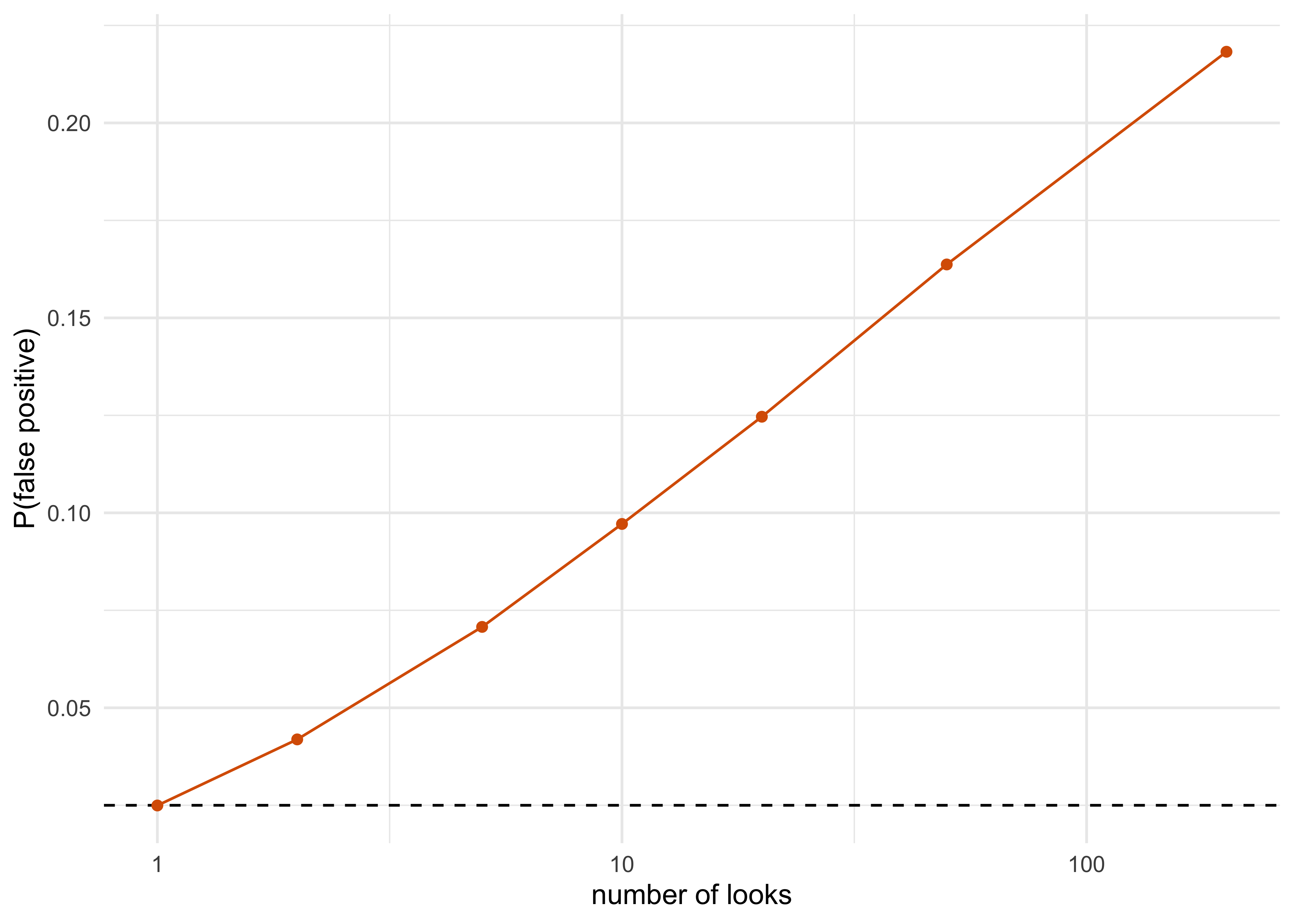
The unplanned look is worth a picture before any theory. Suppose the drug does nothing and a naive analyst applies the ordinary one-sided \(z\) test at the 0.025 level to the accumulating data. How often is a false positive declared if the analyst is willing to look more than once?
Figure 12.1: Probability of at least one false positive when the drug does nothing, as a function of the number of equally spaced looks at 200 observations. The naive z test is applied at the 0.025 level at every look. The dashed line is 0.025.
With a single look the rate is 0.025 (Monte Carlo error aside), with five looks it is 0.071, with twenty it is 0.125, and with a look after every observation it is about 0.22. These are the Armitage, McPherson and Rowe numbers of Chapter 11 reproduced. The rate for the method of this chapter, monitored after every observation, is 0.006. How that is possible is the subject of the next section.
12.2 E-values as bets
The definition
An e-value for a null hypothesis \(H_0\) is a nonnegative random variable \(E\) whose expectation under every distribution in \(H_0\) is at most one, \[
\mathbb{E}_{H_0}[E] \le 1 .
\] An observed e-value of 20 means that the data have multiplied by 20 an amount of evidence that is fair under the null. The name suggests the natural reading: \(E\) is the payoff of a bet. A gambler stakes one dollar against the null (that is, on the drug working), the null being the claim that the bet is fair. If the null is true, the gambler’s expected wealth afterwards is at most one dollar. If the gambler’s wealth ends at \(E = 20\), that outcome was an event which, under the null, has probability at most \(1/20\). This follows from Markov’s inequality, \[
\mathbb{P}_{H_0}(E \ge 1/\alpha) \le \alpha\,\mathbb{E}_{H_0}[E] \le \alpha .
\] So the rule “reject \(H_0\) when \(E \ge 1/\alpha\)” is a level-\(\alpha\) test. At \(\alpha = 0.025\) the threshold is \(E \ge 40\). A fixed-sample e-value is nothing more than a new way of writing a test. The new thing is what happens when the data keep coming.
Test martingales and Ville’s inequality
Now let data arrive in a sequence, and let \(E_n\) be the gambler’s wealth after \(n\) observations, starting from \(E_0 = 1\). Suppose each bet is fair under the null: given the past, the expected wealth after the next observation equals the wealth now. A nonnegative process with this property and \(E_0 = 1\) is called a test martingale (Shafer et al. 2011) (if the expected wealth can only fall, it is a test supermartingale, and everything below holds for it too). Ville’s inequality, the mathematical heart of this chapter, says that such a process crosses a high level only rarely, and that this holds for the entire path, \[
\mathbb{P}_{H_0}\Bigl(\sup_{n} E_n \ge 1/\alpha\Bigr) \le \alpha .
\] The word to notice is \(\sup\). For a fixed \(n\), Markov’s inequality gives the bound at that one time. Ville’s inequality gives the same bound for the supremum over all times, which is the probability that the wealth is ever above \(1/\alpha\). The gambler is allowed to look at the wealth after every patient, to pause and resume, to stop for any reason, including a reason the protocol never considered, and the probability of ever declaring success under the null is still at most \(\alpha\). This is what “anytime-valid” means. For likelihood ratios this bound is the one Wald used for the error rates of his sequential probability ratio test (Wald 1945); Ville’s version (Ville 1939) covers any nonnegative martingale.
NoteTechnical note: why Ville’s inequality holds
Let \(T\) be the first time \(E_n \ge 1/\alpha\) (possibly infinite). The stopped process \(E_{n \wedge T}\) is again a nonnegative martingale, so \(\mathbb{E}[E_{n \wedge T}] = 1\) for every \(n\). On the event \(\{T \le n\}\) the stopped wealth is at least \(1/\alpha\), and it is nonnegative otherwise, so \[
1 = \mathbb{E}[E_{n\wedge T}] \ge \frac{1}{\alpha}\,\mathbb{P}(T \le n).
\] Hence \(\mathbb{P}(T \le n) \le \alpha\) for every \(n\), and letting \(n \to \infty\) gives \(\mathbb{P}(T < \infty) \le \alpha\). The argument is Markov’s inequality applied at the stopping time, with the martingale property supplying the identity \(\mathbb{E}[E_{n \wedge T}] = 1\). Note what is not used: the distribution of the data, the number of looks, and the reason for stopping. The same argument works for a test supermartingale, for which one has \(\mathbb{E}[E_{n \wedge T}] \le 1\).
A betting martingale for a binary endpoint
Take the two-arm binary trial of Sokolova and Sokolov (A. O. Sokolova and Sokolov 2026): patients are enrolled in matched pairs, one to treatment and one to control, and for pair \(i\) let \(D_i = Y_{T,i} - Y_{C,i}\), which equals \(+1\) if only the treated patient responded, \(-1\) if only the control patient responded, and \(0\) otherwise. Under the null that the response probabilities are equal, \(p_T = p_C = p\) for any common value \(p\), we have \(\mathbb{P}(D = +1) = \mathbb{P}(D = -1)\), so \(\mathbb{E}[D] = 0\). Choose a betting fraction \(\lambda \in (0, 1)\) and let \[
E_n = \prod_{i=1}^{n} (1 + \lambda D_i).
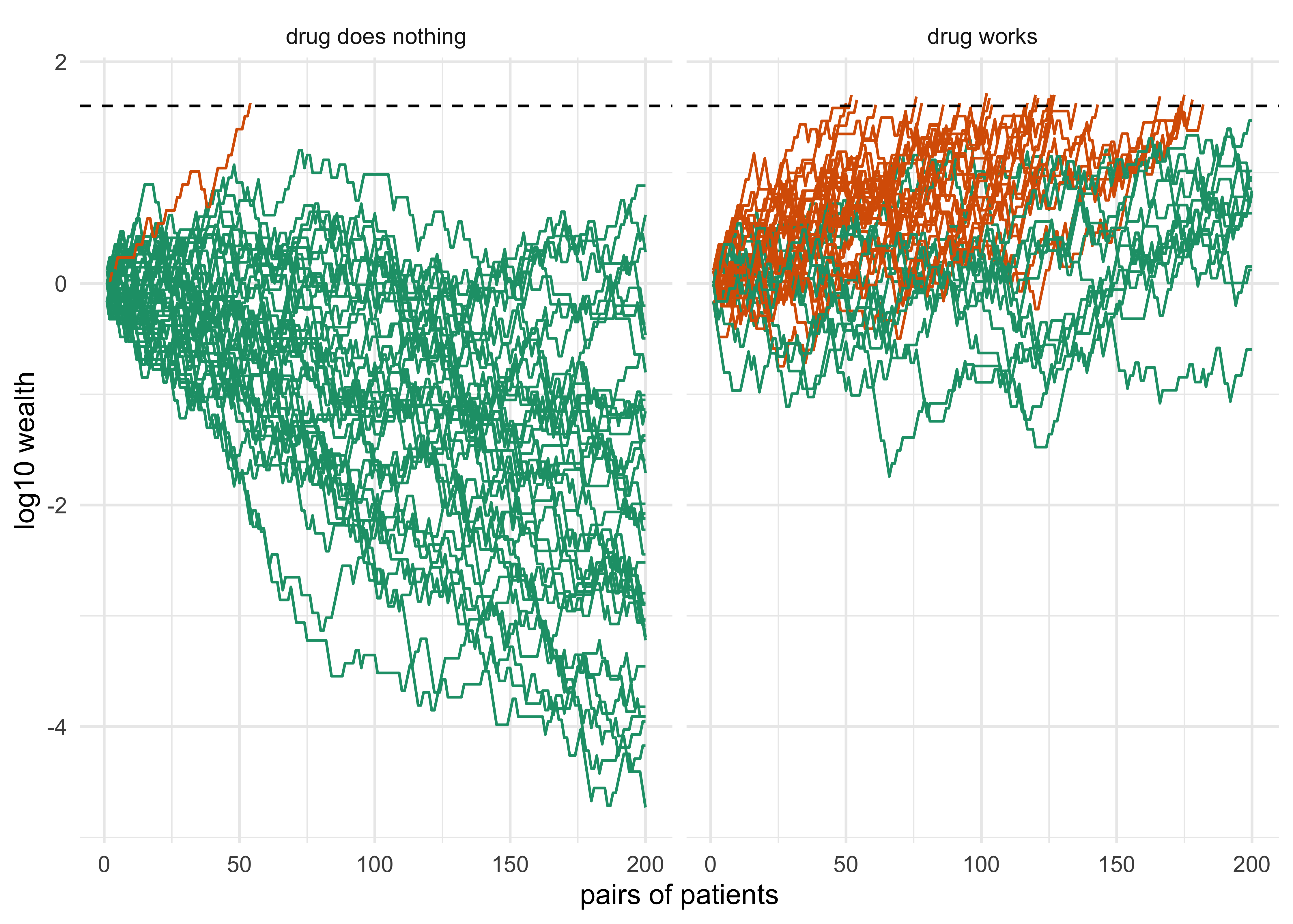
\] Then \(\mathbb{E}[1 + \lambda D_i] = 1\) under the null whatever \(p\) is, so \(E_n\) is a test martingale for the composite null “the two arms have the same response probability”. The nuisance parameter \(p\) never needs to be estimated. In the book’s companion online lab (module 08, https://nytel.ai/testing/08-e-values.html) the paths of this process under the null and under an alternative can be drawn directly. We reproduce the picture.
Figure 12.2: Wealth (log scale) of the betting martingale with fraction 0.31 over 200 pairs, 40 paths per panel. Left: both arms respond at 30 percent, so the null is true and paths drift down. Right: 45 versus 30 percent. Paths are stopped when they reach the dashed line, 1/0.025 = 40, and shown in color.
The left panel shows the feature that surprises people the first time. Under the null the average wealth stays at one dollar, yet the typical path drifts down: the average is held up by rare large excursions, and Ville’s inequality says exactly how rare. The right panel shows what a working drug does: wealth grows, and the path that reaches 40 is declared a success.
With 20,000 simulated trials of 200 pairs the null rate of crossing 40 is 0.017, below the nominal 0.025 (we discuss why in a moment), and when the true rates are 45 and 30 percent about 74 percent of trials cross, with a median crossing at 104 pairs.
How big a bet? The growth rate
A bet that is fair under the null can still be a good or a bad bet under the alternative. If \(\lambda\) is small, wealth grows slowly; if it is large, the wealth wobbles and can collapse. For the binary design above the expected log-growth per pair under the alternative is \[
g(\lambda) = \mathbb{P}(D = +1)\log(1+\lambda) + \mathbb{P}(D = -1)\log(1-\lambda),
\] and the expected number of pairs to reach \(1/\alpha\) is roughly \(\log(1/\alpha)/g(\lambda)\), which is Wald’s identity from the sequential probability ratio test. In the 45 versus 30 percent design of Sokolova and Sokolov the best fraction is \(\lambda^\ast = 0.312\) with \(g = 0.0238\) nats per pair, giving an expected crossing near 155 pairs (A. O. Sokolova and Sokolov 2026). The trade-off is sharp: in their simulations a fraction of 0.10 gives power 0.119, 0.31 gives 0.723 and 0.50 gives 0.589 at 200 pairs. This is the e-value analogue of choosing a design effect size, and it has the same protocol implication: the bet is chosen in advance from the effect one hopes to detect, and an unrealistic choice costs power, not validity. The validity holds for every \(\lambda\).
Cornfield and the betting odds of 1966
The idea is older than the vocabulary. Cornfield (1966a, 1969) proposed what he called relative betting odds as a sequential stopping criterion: the likelihood ratio of the alternative to the null, accumulated as the data arrive and averaged over a prior on the alternative. His companion argument was that the stopping rule should not change the strength of the evidence (Cornfield 1966b). For a simple null the betting odds are a test martingale in the sense of this chapter, so Ville’s inequality bounds the probability that they ever cross a high level, a guarantee that does not need his argument. His proposal lost to alpha spending for a reason that is not statistical. Betting odds require a declared prior on the alternative, and the reviewer has to accept it. The mixture e-value of this chapter makes the same trade, and the regulatory conversation about registering the prior (Chapter 3) is the modern version of that objection.
Shafer and colleagues (Shafer et al. 2011) connect test martingales, Bayes factors and \(p\)-values. Vovk and Wang (Vovk and Wang 2021) develop calibration and combination rules for e-values.
12.3 Likelihood-ratio, mixture and process e-values
Likelihood ratios
When the null and the alternative are each a single distribution, the likelihood ratio \(\prod_i q(Y_i)/p_0(Y_i)\) is a test martingale: under \(p_0\) the expected ratio of densities is \(\int (q/p_0)p_0 = 1\). This is Wald’s SPRT statistic, and for a simple alternative it is the best possible bet in the sense of growth. Its limitation is that it requires committing to one alternative. A bet on a hazard ratio of 0.70 pays badly if the truth is 0.90.
Mixtures
The standard remedy is to average over alternatives. If \(L_n(\theta) = \prod_i p_\theta(Y_i)/p_0(Y_i)\) is a likelihood-ratio martingale for each \(\theta\) in the alternative, then for any mixing distribution \(H\)\[
E_n = \int L_n(\theta)\,dH(\theta)
\] is again a test martingale, because an average of martingales with unit start is a martingale with unit start. For the Gaussian trial of Polson and Sokolov (Polson and Sokolov 2026c), let \(X_i \sim N(\theta, 1)\) denote the standardized treatment-minus-control difference for pair \(i\), \(S_n = \sum_{i\le n} X_i\), and \(H_0:\theta \le 0\). Mixing \(\exp(gS_n - ng^2/2)\) over a half-normal distribution for \(g\) with scale \(\rho\) gives, with \(A_n = n + \rho^{-2}\), the closed form \[
E_n^{+} = \frac{2}{\rho\sqrt{A_n}}\exp\!\Bigl(\frac{S_n^2}{2A_n}\Bigr)\,\Phi\!\Bigl(\frac{S_n}{\sqrt{A_n}}\Bigr).
\tag{12.1}\] For \(\theta < 0\) each integrand is a supermartingale (a martingale at \(\theta = 0\)), so Ville’s inequality holds for the whole composite null. A mirror process, obtained by replacing \(S_n\) with \(-S_n\), monitors the opposite one-sided null and can be used for futility.
The scale \(\rho\) plays the role of a prior standard deviation on the effect: it states how large an effect the bet is hedged against. It is a design parameter and not a nuisance. In the authors’ sweep the integrated Bayes risk of the e-value rule changes by only a few percent across \(\rho\) from 0.10 to 0.32, so the choice matters less than the choice of threshold.
E-processes
Not every sequential statistic is a martingale. Often what one has is a process \(E_n\) that is dominated, under every null distribution, by some test martingale: an e-process. The definitions of this section are enough for the trials in this book, and the distinction matters mainly because it allows e-values to be built for composite nulls and with covariates in cases where no exact martingale exists. For the reader the working rule is the same: if \(\sup_n E_n \ge 1/\alpha\) has probability at most \(\alpha\) under every null, the process can be monitored continuously.
12.4 From e-values to p-values and confidence sequences
A regulator reads a p-value and a confidence interval. An e-process supplies both, in a form that survives continuous monitoring. The always-valid p-value after \(n\) observations is \[
p_n = \min\Bigl(1, \frac{1}{\max_{m\le n} E_m}\Bigr).
\] It is nonincreasing in \(n\), it can only improve as evidence accrues, and \(\mathbb{P}_{H_0}(\inf_n p_n \le \alpha) \le \alpha\): the probability that the always-valid p-value is ever below \(\alpha\) is at most \(\alpha\). For a fixed-sample e-value the same relation, \(p = \min(1, 1/E)\) (with \(p = 1\) when \(E = 0\)), is a valid but conservative p-value by Markov’s inequality, and the conservatism is part of what is paid. A running maximum of 15.3 gives \(p = 0.065\), a running maximum of 45.8 gives \(0.022\). These are the numbers from the reanalysis of the Novick and Grizzle ulcer trial in Sokolova and Sokolov (A. O. Sokolova and Sokolov 2026), where the e-value of surgery A versus B is 15.3 and A versus C is 45.8 (these are the e-values of that paper’s dataset, not computed from the ulcer data table of Chapter 10, and the patient order is simulated because the original order is not recorded; this is an illustration and not a valid test of that trial).
A confidence sequence is the interval analogue. It is a sequence of intervals \(C_n\) such that \(\mathbb{P}(\theta \in C_n \text{ for all } n) \ge 1-\alpha\), constructed by inverting the e-process over null values, and the idea goes back to the confidence sequences of Darling and Robbins (Darling and Robbins 1967; Robbins 1970), studied further by Lai (Lai 1976), and its group sequential counterpart in clinical trials is the repeated confidence interval of Jennison and Turnbull (Jennison and Turnbull 1984). A confidence sequence is wider than a fixed-sample confidence interval at the same \(n\), and it can be read at any time, including at the time the DMC stopped the trial. The estimation principle in the Adaptive Designs guidance, that estimates be “sufficiently reliable”, is what the confidence sequence is for.
12.5 The surcharge: what validity at every stopping time costs
The exact tolls and their derivation are in Chapter 11 (Equation 11.8, Table 11.6); this section only identifies the construction and the comparison baseline. The e-process rule at level \(\alpha\) is the symmetric normal-mixture Bayes factor with \(b = 1/\alpha\), with \(q = I_n\tau^2\): the log of the symmetric normal-mixture e-value is \(\tfrac12\{qZ_n^2/(1+q) - \log(1+q)\}\), so for a one-sided claim (\(Z_n > 0\)) it acts when \(Z_n^2 \ge (1+1/q)\{\log(1+q) + 2\log(1/\alpha)\}\), which exceeds the Bayes bar at \(b = 1\) by \(2\log(1/\alpha)(1+1/q)\), approximately \(2\log 40 = 7.38\) at large information. The half-normal mixture of Equation 12.1 has the exact log e-value \(\log 2 + \tfrac12\{qZ_n^2/(1+q) - \log(1+q)\} + \log\Phi\bigl(Z_n\sqrt{q/(1+q)}\bigr)\); at large information the correction reduces to \(\log 2\), which lowers the bar by about \(2\log 2 = 1.39\). The baseline is the uncalibrated Bayes-factor bar (posterior odds of one). The resulting figure of about seventy percent of a conventional trial (Equation 11.11) compares boundary terms asymptotically and is not an exact sample-size identity, and it is a cost of this construction, not of anytime validity in general (iterated-logarithm boundaries (Robbins 1970) behave differently). Calibration narrows it, as the SELECT comparison below shows. The figure is also not a statement that a sponsor who adopts an e-value design will run a trial 70 percent longer than a fixed design: stopping early at a large effect is built into the e-value design.
12.6 E-values and Bayes factors
The mixture e-value (Equation 12.1) looks like a Bayes factor, and it is one: it is the ratio of the marginal likelihood under a half-normal prior on the effect to the likelihood at the null value. The two ideas share their statistic and differ in how the statistic is read.
A Bayes factor \(\mathrm{BF}_{10}\) is read as a measure of evidence, on the scale of Jeffreys’s table, or combined with prior odds to give a posterior probability. For a simple null, \(\mathbb{E}_{H_0}[\mathrm{BF}_{10}] = 1\), so a Bayes factor is an e-value (Shafer et al. 2011; Shafer and Vovk 2019).
An e-value is read as a test statistic with a guaranteed error rate: reject when it exceeds \(1/\alpha\). The calibration is fixed by Markov’s and Ville’s inequalities and does not need a prior.
So the same number, say 40, is “strong evidence” on a Jeffreys scale and “a level 0.025 test” on the e-value scale. That is the sense in which the difference is one of calibration and not of statistic. A Bayes factor of 3 is a Bayes factor and an e-value of 3; it supports the alternative, but rejecting at 3 has a frequentist type I error as high as \(1/3\). The Bayesian reading is not wrong, it answers a different question, and Chapter 7 discussed which.
Two caveats. With a composite null, a Bayes factor with a prior on the null parameter is not an e-value in general, because its expectation is only an average under the null prior. And most e-values are not Bayes factors: the betting martingale of the binary trial multiplies \(1 + \lambda D_i\), which is a likelihood ratio against no particular prior. The e-value framework is wider than Bayes factors, and the Bayes factor is the particular e-value that is calibrated for the prior used to mix it.
Polson and Sokolov (Polson and Sokolov 2026b) push the observation further. Their theory companion shows that the loss-optimal rejection boundary on the standardized scale grows like \(\sqrt{\log n}\) (the moderate deviation scale), that the \(1/\alpha\) rule is a fixed worst-case bound on a different (large deviation) scale, and that the Bayes factor is the e-variable calibrated at the first of these. The practical content is the next section: the statistic can be the same and the threshold different, and the threshold is where most of the cost lies.
12.7 Power and stopping time: e-value, Bayesian and group sequential designs
There are two comparisons, one on a binary endpoint (A. O. Sokolova and Sokolov 2026) and one on a time-to-event endpoint that reconstructs the SELECT trial of semaglutide (Polson and Sokolov 2026a). They produce different power orderings, and the difference is instructive. For SELECT there is one set of numbers in this book, those of the full reconstruction in Table 12.2.
Two-arm binary design
The design of Sokolova and Sokolov (A. O. Sokolova and Sokolov 2026) has \(H_0: p_T = p_C = 0.30\) against \(H_1: p_T = 0.45\), 1:1 randomization, at most 200 pairs, twenty looks every ten pairs, one-sided \(\alpha = 0.025\), 50,000 replications. Table 12.1 reproduces their results. All figures are from their Table 2 and Table 5; we have not re-simulated them.
Table 12.1: Binary two-arm trial, 20 looks at 10 pair intervals, from Sokolova and Sokolov (A. O. Sokolova and Sokolov 2026).
Method
Type I error
Power
Mean n under null
Mean n under alternative
E-value betting (\(\lambda = 0.31\))
0.012
0.723
199.0
139.2
Group sequential, boundary \(c/\sqrt{t}\), calibrated
0.025
0.861
198.9
139.8
Calibrated Bayesian posterior
0.020
0.688
197.1
133.9
Naive repeated p-values
0.148
0.933
178.4
74.2
Naive posterior threshold 0.975 (Jeffreys)
0.135
0.932
181.0
76.2
Three things stand out. The two naive rules are fast and powerful because their type I error is 14 percent: this is the repeated-look inflation of the first figure, and the table makes clear that a speed comparison means nothing unless the type I error is reported next to it. A naive posterior probability threshold of 0.975 under continuous monitoring is not safe either: the same inflation appears in the Bayesian column, a point we repeat in Chapter 14. Second, once each rule is calibrated, the group sequential design has the highest power (0.861), the e-value rule is next (0.723), and the calibrated Bayesian rule is last (0.688), stopping slightly earlier on average (133.9 against 139.2) but reaching its bar less often. Third, the e-value rule is conservative: its realized type I error is 0.012, about half the nominal level, because Ville’s inequality is not tight: the wealth process overshoots the boundary when it crosses, so the bound is attained only in the limit of paths that stop exactly at the level, and a finite horizon leaves noncrossing some paths that would eventually have crossed.
Sokolova and Sokolov also vary the look schedule. With five planned looks the group sequential power is 0.870 against 0.686 for the e-value rule. With twenty looks it is 0.861 against 0.723. With five looks at random times it is 0.868 against 0.679. With continuous monitoring the e-value rule is at 0.750 and the group sequential design is not compared, because its boundary is not designed for 200 looks. The qualitative message is the one that matters: when the schedule is known and kept, the group sequential design is more powerful by 14 to 19 points of power in this design; the e-value rule keeps working when the schedule is not known.
Time-to-event design: the SELECT reconstruction
Polson and Sokolov (Polson and Sokolov 2026a) reconstruct SELECT, the cardiovascular outcomes trial of semaglutide (Lincoff et al. 2023), as a counterfactual: a Gaussian approximation in event time with a true hazard ratio held at the observed 0.80 (SELECT itself was designed for 0.83, at 90% power, with 1,225 planned events and one superiority interim at two thirds of them (Ryan et al. 2020)), a normal prior of scale \(\tau = 0.25\) on the log hazard ratio, and a trial that ends at 1,270 events. Three rules are compared at a nominal 2.5 percent type I error under their own monitoring (the O’Brien-Fleming boundary and the Bayesian threshold are calibrated to it, and the e-value rule is bounded by it through Ville’s inequality, with a lower realized rate): a four-look O’Brien-Fleming design at 25, 50, 75 and 100 percent of the events; the e-value mixture (the symmetric normal mixture, whose bar exceeds the Bayes bar by about the surcharge \(2\log 40 = 7.38\)), continuous, \(E \ge 40\); and the continuous Bayesian posterior rule with a threshold raised until the type I error is 2.5 percent. For comparison the table includes SELECT’s planned design: interim at 817 of 1,225 events, Lan-DeMets O’Brien-Fleming-type spending, then the final analysis, with nominal one-sided levels of about 0.00606 and 0.0231. Crossing a boundary is necessary but not sufficient for stopping: the DMC continued SELECT at its actual 831-event interim. We run the reconstruction with select_simulate() from the package, 40,000 simulated paths per hypothesis, and it is the only SELECT comparison used in this chapter; Chapter 21 returns to it and compares it with the authors’ own script. The posterior bar that gives 2.5 percent is \(p^\ast\) = 0.9952, against a naive type I error of 11.8 percent if the posterior were simply required to exceed 0.975 under continuous monitoring.
Show the R code
knitr::kable(data.frame(Rule =c("O'Brien-Fleming, four scheduled looks", "E-value mixture, continuous, $E \\ge 40$", "Bayes posterior, continuous, calibrated $p^\\ast$", "SELECT planned design (interim at 817 of 1,225 events, Lan-DeMets OBF-type spending, then final)"),"Median events, declaring efficacy"= sr$median_events_success, "Median events, all trials"= sr$median_events_all, Power =sprintf("%.1f%%", 100* sr$power),"Realized type I"=sprintf("%.2f%%", 100*c(sel$gs_typeI, sel$ev_typeI, sel$bayes_typeI, sel$actual_typeI)), check.names =FALSE), align ="lrrrr")
Table 12.2: SELECT reconstruction (true hazard ratio 0.80, a counterfactual; tau = 0.25; at most 1,270 events for the first three rules; 40,000 paths, seed 31415). Medians are given among trials that declare efficacy and over all trials, where a trial that never crosses is counted at its final read-out. Power is the probability of acting; realized type I is under the null at the rule’s own monitoring.
SELECT planned design (interim at 817 of 1,225 events, Lan-DeMets OBF-type spending, then final)
817
817
97.4%
2.54%
The ordering by stopping time is the clear result. Among simulated trials that declare efficacy, the median stopping point is 464 events for the Bayesian rule, 612 for the e-value rule and 952 for the four-look O’Brien-Fleming design, against 817 for SELECT’s planned two-look design. Over all trials, counting those that never cross at the 1,270-event read-out, the medians are 486, 714 and 952. The powers sit beside them: 94.7 percent for the Bayesian rule, 83.1 for the e-value rule, 97.7 for the four-look design and 97.4 for SELECT’s planned design. The Bayesian rule is calibrated to 2.5 percent, and the e-value rule is conservative, with a realized type I error of 0.58 percent against a nominal 2.5. The unadjusted single look at \(z = 1.96\) would cross at about 309 events on the mean path (from \(Z = |\log 0.80|\sqrt{d}/2\)), earlier than the calibrated Bayesian rule, which is the arithmetic that the thesis of this book requires us to acknowledge. Against the calibrated Bayesian rule the e-value rule needs 32 percent more events at the median among trials that declare efficacy. That is the realized price of validity at every stopping time once the Bayesian rule is calibrated, in this construction, and it is smaller than the asymptotic seventy percent measured against the uncalibrated Bayes-factor bar. The stopping times are events in a modeled counterfactual; any conversion to calendar time, patient-years or cost would inherit the same conditioning.
Why the orderings differ
The two comparisons give power orderings that appear to contradict each other. In the SELECT-like trial the calibrated Bayesian rule has more power than the e-value rule (94.7 against 83.1 percent in Table 12.2). In the binary trial it has less (68.8 against 72.3 percent). Both can hold, and the following are the plausible contributors, which neither Sokolova and Sokolov nor Polson and Sokolov isolates.
Prior scale relative to the effect. In SELECT the effect (a hazard ratio of 0.80) is of a plausible size relative to a prior with \(\tau = 0.25\), so the calibrated Bayesian bar (the \(Z\) bar implied by \(p^\ast\), which is above the uncalibrated \(\sqrt{L_n}\)) is low relative to the realized \(Z_n\) (about 4 at the end). In the binary design the effect is modest relative to the information, and the Bayes bar is not much below the e-value bar.
Conservatism of the e-value. The e-value rule’s realized type I error is 0.58 percent in the SELECT design and 1.2 percent in the binary design, against a nominal 2.5. Some of the lost power is spent on that unused budget, and the amount depends on the design.
The endpoint. Time-to-event data accumulate on an information scale where \(L_n\) is modest (\(3.0\) at 1,270 events with \(\tau = 0.25\)) and slowly growing, while the binary trial is small and its likelihood ratio has a different shape.
Polson and Sokolov (Polson and Sokolov 2026a) conclude that the robust finding across both studies concerns stopping time, not power, and that the direction of the power difference should be checked for the design at hand. We agree. In the language of Chapter 14, this is a statement that the operating characteristics have to be simulated for the specific design, and no theory replaces that report.
12.8 What a Bayes-risk comparison adds
The comparison so far is by type I error, power and stopping time, which are the currency of regulators. A different comparison asks what each rule costs in patients, and the working paper of Polson and Sokolov (Polson and Sokolov 2026c) makes it for a stylized mortality-type problem. Each pair is \(N(\theta, 1)\) with a prior \(\theta \sim N(0, 0.15^2)\), at most 1,000 pairs, a post-trial population of \(M = 20{,}000\) patients, and a loss equal to \(M|\theta|\) if the wrong terminal decision is made, plus \(|\theta|\) per enrolled pair. The effect \(\theta\) is a standardized effect, which is not an absolute mortality-risk difference, so the losses below are in illustrative loss units, not literal deaths; reading them as deaths would need a mortality scale and a conversion from the standardized effect. Relative reductions within the stipulated loss model are meaningful as they stand. The Bayes-optimal rule is computed by backward induction on the sufficient statistic \((n, S_n)\) (Chapter 15). The e-value rule is \(E_n^{+} \ge 40\) with the mirror process for futility. We report their numbers, which we have not re-run.
Neither rule dominates. The risk functions cross. For marginally harmful treatments (\(\theta \in [-0.05, -0.015]\)) the e-value rule has the lower expected loss, because its bar of 40 almost never approves a harmful drug (approval probability at most 0.006, against 0.333 for the Bayes rule at \(\theta = -0.015\)). For beneficial treatments the Bayes rule is far better: at \(\theta = 0.07\) the e-value rule approves 32.7 percent of the time against 98.2 percent, runs on average 849 pairs against 412, and has an expected loss of 1,001 against 55 loss units. The e-value rule is underpowered for effects of that size in a trial of 1,000 pairs.
Integrated Bayes risk. Averaged over the prior, the Bayes rule has an expected loss of 53.4 loss units and the e-value rule 237.6, a reduction of 77.5 percent (Monte Carlo standard errors 1.0 and 3.1). The reduction stays between 71 and 82 percent for horizons from 500 to 2,000 pairs, and widens as the stakes rise: 73.1 percent at \(M = 10^4\) and 84.4 percent at \(M = 10^5\). This is by construction, since the Bayes rule minimizes this criterion. It does not say that the Bayes rule is better by the criterion of a regulator.
Where the gap comes from. The gap decomposes into two parts. A rule that monitors the same e-process but stops at the loss-optimal threshold (\(E^{+} \ge 3.5\)) instead of \(E^{+} \ge 40\) has Bayes risk 118.3, so recalibrating the threshold closes 119.3 of the 184.2 loss-unit gap (64.8 percent), and the remaining 35.2 percent is the value of the sampling-cost-aware continuation region. In the words of the authors, the e-process statistic is sound; it is the \(1/\alpha\) calibration that carries most of the loss.
A caveat on the hybrid rule. The working paper recommends the loss-tuned rule as a default for a sponsor unwilling to give up validity. That recommendation needs care. By Ville’s inequality a threshold of 3.5 bounds the type I error by \(1/3.5 \approx 0.29\), so the tuned rule does not keep the 2.5 percent guarantee at its tuned threshold; what it keeps is the validity of the always-valid p-value computed from the same process, which can still be reported even if the trial is stopped on a different, loss-based criterion. A rule that keeps both the 2.5 percent guarantee and the loss-based stopping is the open problem the authors identify: a monitoring rule that is anytime-valid and calibrated to the moderate deviation scale at its realized stopping time.
The same paper makes a large-scale comparison, e-BH against empirical Bayes in 2,000 simultaneous tests with 5 percent signals: the e-BH procedure has a false discovery rate of 0.002 and power 0.174, while an empirical-Bayes rule that targets an FDR of 0.10 has FDR 0.098 and power 0.317. It is not a trial-level comparison and we note it only as a statement of the same pattern, robustness paid for in efficiency (see Chapter 10 for the multiplicity machinery the reader will meet in a trial).
12.9 When should a sponsor pay the surcharge?
The design question is not Bayesian against frequentist in the abstract, but whether the trial needs validity at stopping times the protocol cannot anticipate (Polson and Sokolov 2026a). If it does, the surcharge \(2\log(1/\alpha)\) is the price, worth about seventy percent of a conventional trial by Equation 11.11 against the uncalibrated Bayes-factor bar (the realized gap to a calibrated Bayesian rule is smaller, 612 against 464 events among SELECT-reconstruction trials that declare efficacy), and it belongs in the sample size justification as an explicit line and not as a footnote about anytime validity. The advice of Polson and Sokolov is to itemize the toll before choosing the paradigm. A practical test has five questions.
Is the monitoring schedule under the sponsor’s control and will it be kept? If the DMC charter fixes the looks and the committee will not deviate, a classical group sequential design is the more powerful choice (86 against 72 percent in the binary example), and the sponsor should not pay the surcharge.
Is a continuously monitored or open-ended decision part of the design? Platform trials with continuous or frequent interim reviews, adaptive enrichment with open-ended expansion, and trials whose end is defined by a data-driven event are the natural cases for an anytime-valid design. In Chapter 20 the reader will see that arm-level decisions in a platform repeat the same question many times.
Can the sponsor foresee the plausible unplanned looks? If an external readout, a safety review or an extension is likely, a classical design can, in part, accommodate it by pre-specification (a spending function, a pre-specified sample size re-estimation). If the sponsor cannot enumerate them, the e-value design is insurance.
Is there a reason to expect off-schedule looks that the protocol cannot list? An e-process protects against optional stopping, whatever the schedule, under its assumptions. It does not repair bias from unblinding, altered endpoint assessment, selective data collection or invalid model changes, so confidentiality and conduct safeguards are as necessary for an e-process design as for a group sequential one. A sponsor whose DMC has a history of ad hoc looks may still judge that a guarantee that does not depend on the look schedule is worth the price.
Can the sponsor live with the power cost? The cost is real. In the binary example the e-value rule lost 14 points of power to a group sequential design that knew its schedule, and in the Bayes-risk comparison the e-value rule is far behind for modest effects. Restoring it means a larger horizon or a better process while keeping the efficacy threshold at 40. A loss-based stopping decision, such as the threshold of 3.5 in the Bayes-risk comparison, does not itself establish efficacy at 0.025, and reporting the e-process p-value beside it does not restore that guarantee for the decision.
If the answers to the first and third questions are yes, do not pay. If the answers to the second and fourth are yes, pay and say so in the sample size section. If the answers are mixed, the middle route is a protocol that keeps a group sequential or Bayesian design as the primary analysis, with an e-process monitored in parallel as an always-valid ledger. Sokolova and Sokolov suggest exactly that: run the e-process alongside a Bayesian rule and report the e-value, its always-valid p-value and a confidence sequence as a frequentist evidential record of the trial (A. O. Sokolova and Sokolov 2026). The primary analysis is not displaced, and the ledger answers the inevitable question about the unplanned look.
There is also a Bayesian answer to optional stopping that does not concede the point: posterior and predictive probabilities condition on the data actually observed, so a Bayesian analysis is coherent regardless of when or why the data were examined, and the stopping rule does not enter the posterior (A. Sokolova, Sokolov, and Polson 2026). That is true of the posterior. It is not true of a decision rule that has been calibrated to type I error under a stated monitoring scheme, which is the route this book takes as its default for confirmatory designs without borrowing (one of the routes the FDA draft describes), and the calibration is the part that does not survive a deviation. The Bayesian rule of the SELECT comparison holds 2.5 percent under the scheme it was calibrated to and some other number under another scheme. The two paradigms make different promises, and the comparison of the SELECT table is a comparison under the Bayesian’s assumptions. The e-value rule trades some of the efficiency for a promise that does not need that assumption.
Many subgroups at once: a negative result for the mixture e-value
An e-value looks attractive when the analysis choices cannot be enumerated, as in the garden of forking paths of Section 10.3, because a mixture over a prespecified family of \(K\) candidate analyses is a valid e-value for the global null that all candidate subgroup effects are nonpositive. Rejecting it does not establish efficacy in a selected subgroup, and subgroup-specific claims need an appropriate multiplicity procedure. When \(K\) is known, declared and fixed, the comparison is with the Sidak-corrected maximum, and the answer is mixed. We simulate \(K = 20\) standardized statistics with equicorrelation \(\varrho\), and compare the naive rule (report the largest, test at 0.025), the Sidak maximum, and the equal-weight mixture e-value \(\bar e = K^{-1} \sum_k 2(1+\lambda^2)^{-1/2} \exp\{\lambda^2 Z_k^2 / (2(1+\lambda^2))\}\,\mathbb{1}\{Z_k > 0\}\) with \(\lambda^2 = 9\) at the threshold \(1/\alpha\). The indicator makes the mixture a positive-direction (one-sided) e-value, so that the maximum and the mixture test the same alternative, a positive effect in at least one subgroup; the squared symmetric form would also spend power on negative effects. Power is compared at thresholds recalibrated to realized size 0.025.
Table 12.3: K = 20 equicorrelated subgroup statistics, 200,000 replicates, positive-direction mixture with prior scale lambda^2 = 9. Upper block: realized type I error at each rule’s nominal threshold under the global null. Lower block: power at thresholds recalibrated to realized size 0.025.
rho
Naive
Sidak
Mixture e-value
0.0
0.397
0.024
0.0007
0.5
0.211
0.018
0.0010
0.8
0.113
0.009
0.0012
Scenario
rho
Sidak
Mixture e-value
one effect d=3.0
0.0
0.505
0.506
one effect d=3.5
0.0
0.694
0.694
three effects d=2.5
0.0
0.669
0.730
five effects d=2.2
0.0
0.693
0.795
one effect d=3.0
0.5
0.541
0.425
one effect d=3.5
0.5
0.725
0.612
three effects d=2.5
0.5
0.584
0.503
five effects d=2.2
0.5
0.554
0.500
The naive rule is as bad as advertised: it approves a useless drug 40 percent of the time at \(\varrho = 0\). The mixture e-value at its nominal threshold is very conservative, with realized size at most 0.0012 against a nominal 0.025, because Markov’s inequality is loose for a single look. Recalibrating to matched size removes that penalty. With no correlation and several true effects the positive-direction mixture is at least as powerful as Sidak (0.80 against 0.69 for five effects at \(\varrho = 0\)), because it pools evidence across the true effects, while for a single effect the two tie (0.51 against 0.51). Under correlation \(\varrho = 0.5\) the maximum wins in every scenario, by 0.05 to 0.12. The reading is therefore narrow: the mixture is competitive when several subgroups carry effects and the statistics are nearly independent, and loses when they are correlated.
What this licenses is limited. It does not say mixture e-values dominate multiplicity corrections, nor that they are dominated, and the simulation covers one fixed look at known \(K\) and a few configurations. The mixture displayed here is a fixed-look e-value: it has no time index and no prespecified construction for further analyses, so its guarantee holds at the single look at which it is computed. Applying its constant threshold repeatedly to standardized cumulative data would cross under the null with probability one eventually. Validity under continued monitoring, or continuation into a second cohort, would need component e-processes with prespecified weights and a proof of their joint monitoring guarantee, which is not shown here. The Sidak guarantee also needs \(K\) declared and fixed. The guarantee is never free, and what a mixture buys beyond the maximum is a way to weight prespecified analyses, not an answer to unlisted ones.
12.10 What the regulator will ask
No guidance names e-values, so the sponsor is arguing from principle. The principle is available and it is the one the Adaptive Designs guidance and E20 state: the chance of erroneous conclusions should be adequately controlled, the design should be completely prespecified, and the trial’s integrity should be maintained. An e-value design satisfies the first under its assumptions: the type I error is at most \(\alpha\) for every stopping time, which is stronger than the guidance asks. That protection is against optional stopping; it does not repair bias from unblinding, altered endpoint assessment, selective data collection or invalid model changes. It satisfies the second in a particular way: what is prespecified is the e-process, the mixing distribution (or betting fraction), the threshold and the horizon, and not the look schedule. On the third, it removes the statistical consequence of an off-schedule look but not the need for the same confidentiality and conduct safeguards that a group sequential design requires.
What will not be familiar to the reviewer is the machinery, so the submission has to carry what a standard SAP would not: a statement of the null hypothesis as a composite null for which the process is a test supermartingale, the proof (or a reference) that the process is one, the choice of \(\rho\) or \(\lambda\) with its justification from the target effect, a simulation report showing type I error and power over the scenarios of interest (the same report as Chapter 14, with the difference that the type I error is expected to be below nominal and the report should say by how much), and the always-valid p-value and confidence sequence in the format of the CSR. The FDA’s CID paired meeting program and the Type B and C meetings described in Chapter 3 are the forum. A sponsor should also expect the question “why not a spending function?”, and the answer is the five-question test above, not a general preference.
TipIn the protocol
Wording a sponsor could adapt for the statistical section of a protocol that uses an e-process, to be agreed with the agency in advance:
“The primary analysis is a mixture e-process \(E_n^{+}\) for the null hypothesis \(H_0:\theta \le 0\), defined in Appendix X with mixing distribution half-normal with scale \(\rho = \dots\). The null hypothesis is rejected, and the trial may stop for efficacy, at the first interim review at which \(E_n^{+} \ge 40\). By Ville’s inequality the probability under \(H_0\) that \(E_n^{+}\) ever exceeds 40 is at most 0.025, irrespective of the number and timing of reviews. Always-valid p-values \(p_n = \min(1, 1/\max_{m\le n}E_m^{+})\) and a 95 percent confidence sequence for \(\theta\) will be reported in the clinical study report at the time of the final analysis. The operating characteristics under the design scenarios (Section Y) are those of the simulation report.”
12.11 In practice
No trial has yet been run on an e-process as its primary analysis, and no regulator has said anything about the method. What real trials do offer is the situation the chapter is about: a monitoring schedule that was fixed in advance, and the question of what would have happened had it not been.
BNT162b2: several interim looks on a schedule fixed in the SAP
The phase 3 trial of the Pfizer and BioNTech COVID-19 vaccine (Protocol C4591001, NCT04368728) is a clear example of a Bayesian design with several interim looks, prespecified before the relevant unblinded analyses (Pfizer Inc. 2022). The linked document is a later amended version of the SAP (version 10, dated 7 October 2022), so it documents the rules but does not by itself establish their chronology. The model, prior, thresholds and the clinical result are in Section 21.5, and the worked posterior computation is in Chapter 6. What matters here is the schedule: the final analysis was planned at 164 primary cases, with interim looks planned at 32, 62, 92 and 120 cases and posterior thresholds of 0.995 at an interim analysis and 0.986 at the final one, calibrated to an overall one-sided type I error of 2.5 percent. According to the SAP the look at 32 cases was not performed; the remaining three looks and the thresholds were unchanged, and the SAP states that the overall type I error stays at 0.025.
The lesson for this chapter is about what the design needed and what it did not. The number of looks and the threshold at each were fixed before the first case, so the group sequential-type guarantee held and a method that is valid at every stopping time was not needed; a sponsor in this position should not pay the surcharge. The case supports prespecified decision rules. It does not show that an unlisted case count necessarily breaks validity: FDA’s statistical review (section 6.1.9) reports that the first interim analysis actually performed was at 94 cases and the final analysis at 170, not at exactly the listed 92 and 164, which is the ordinary operational overrun between a planned trigger and the realized data cut. Distinguishing planned triggers from exact analysis counts matters: whether an analysis at a realized count differing from the plan stays within the type I error guarantee depends on whether the thresholds were defined on the planned counts or adjusted to the realized information, and that is a rule the SAP must state. The thresholds of 0.995 and 0.986 are a bar calibrated for the planned looks (four interim looks plus the final analysis), and the SAP’s own handling of the dropped first look (the thresholds were kept) can only lower the type I error, since removing a look with unchanged thresholds shrinks the rejection region. An e-process monitored alongside would have supplied a validity statement that does not depend on the schedule.
Key points
A classical group sequential design controls the type I error as a property of its plan. Unplanned looks that depend on the accumulating comparative results, data-dependent looks under a fixed boundary schedule, continuous DMC review and extensions of the trial are outside that plan, while independent external triggers such as a publication can be accommodated if the monitoring rule is valid at arbitrary times, as an e-value rule is. For each the question is whether the request used accumulating comparative results and whether the spending or adaptation method remains valid.
An e-value is a nonnegative statistic with expectation at most one under the null. A test martingale is a nonnegative process starting at one whose next value has conditional expectation equal to its current value under every null distribution (replacing equality by an upper bound gives a test supermartingale), and Ville’s inequality bounds the probability that it ever exceeds \(1/\alpha\) by \(\alpha\), for every stopping time.
Likelihood ratios and mixtures of them are test martingales. The always-valid p-value is \(1/\max E_m\) and a confidence sequence is the matching interval.
The same statistic is a Bayes factor (read as evidence) or an e-value (read with the threshold \(1/\alpha\) as a level-\(\alpha\) test). The difference is calibration, not statistic.
For the normal-mixture e-value, the approximate price of validity at every stopping time is the surcharge \(2\log(1/\alpha) = 7.38\) in squared standardized evidence (exactly \(7.38(1+1/q)\)), about 70 percent of a conventional trial against the uncalibrated Bayes-factor bar, as a comparison of boundary terms; it is not a universal cost of anytime validity. Calibration narrows it (SELECT reconstruction, among trials that declare efficacy: 464 events for the calibrated Bayesian rule, 612 for the e-value rule). The Bayes-factor bar is itself above a single unadjusted look once \(I_n\tau^2 > 46\) asymptotically.
The orderings are design-dependent: group sequential with a known schedule has the most power at full information; the calibrated Bayesian rule stops first; the e-value rule is conservative. The power ordering of Bayes and e-value reversed between the two studies’ designs, and the stopping-time ordering did not.
No FDA or ICH guidance names e-values as of November 2026. The argument is the type I error control principle of the Adaptive Designs guidance and E20, made in a CID-type interaction.
Pay the surcharge when the trial needs validity at looks the protocol cannot anticipate, and say so in the sample size justification.
NoteDiscussion questions
A DMC charter lists four looks. In the middle of the trial a competing trial reads out and the committee requests a fifth, unscheduled look. What does a Lan-DeMets spending function allow, what does it not allow, and what would an e-process add? What would a regulator ask to know about why the look was requested?
The always-valid p-value after a running maximum of \(E = 15.3\) is 0.065. A reader says this is “not significant” and a colleague says the evidence is “fifteen-fold”. Who is right, and what does each statement mean?
The surcharge in information is about 70 percent of a conventional trial (against the uncalibrated Bayes-factor bar). A sponsor says: “we will never look more than twice, so the surcharge is wasted.” Is that argument correct? What would change it?
In the binary design the calibrated Bayesian rule has less power than the e-value rule, and in the SELECT-like design it has more. Name two properties of the designs that could explain the reversal, and say what simulation you would run to check them for your own trial.
The loss-tuned e-value rule with a threshold of 3.5 halves the Bayes risk of the default. What does it do to the type I error guarantee, and how could the sponsor report the trial honestly?
TipTry it in the lab
Open module 08 at https://nytel.ai/testing/08-e-values.html. Before pressing anything, predict how many of 40 trials with a drug that does nothing will cross the $40 line, then count them; then press “RECOVERY-like” and predict, and check, what fraction of trials with RECOVERY’s survival rates (77.1 versus 74.3 percent, 2,000 per arm) reach $40.
Cornfield, Jerome. 1966a. “A Bayesian Test of Some Classical Hypotheses, with Applications to Sequential Clinical Trials.”Journal of the American Statistical Association 61 (315): 577–94. https://doi.org/10.1080/01621459.1966.10480890.
Darling, D. A., and Herbert Robbins. 1967. “Confidence Sequences for Mean, Variance, and Median.”Proceedings of the National Academy of Sciences 58 (1): 66–68. https://doi.org/10.1073/pnas.58.1.66.
Jennison, Christopher, and Bruce W. Turnbull. 1984. “Repeated Confidence Intervals for Group Sequential Clinical Trials.”Controlled Clinical Trials 5 (1): 33–45. https://doi.org/10.1016/0197-2456(84)90148-X.
Lincoff, A. Michael, Kirstine Brown-Frandsen, Helen M. Colhoun, John Deanfield, Scott S. Emerson, Sille Esbjerg, Soren Hardt-Lindberg, et al. 2023. “Semaglutide and Cardiovascular Outcomes in Obesity Without Diabetes.”New England Journal of Medicine 389 (24): 2221–32. https://doi.org/10.1056/NEJMoa2307563.
Polson, Nicholas G., and Vadim Sokolov. 2026a. “Bayesian Versus Standard Clinical Trial Design: Theory, Evidence, and Protocol.”
———. 2026b. “E-Values on the Moderate Deviation Scale.”
———. 2026c. “Sequential and Large-Scale Decision-Making in Clinical Trials: E-Values Versus Bayes Risk.”
Robbins, Herbert. 1970. “Statistical Methods Related to the Law of the Iterated Logarithm.”The Annals of Mathematical Statistics 41 (5): 1397–1409. https://doi.org/10.1214/aoms/1177696786.
Ryan, Donna H., Ildiko Lingvay, Helen M. Colhoun, John Deanfield, Scott S. Emerson, Steven E. Kahn, Robert F. Kushner, et al. 2020. “Semaglutide Effects on Cardiovascular Outcomes in People with Overweight or Obesity (SELECT) Rationale and Design.”American Heart Journal 229: 61–69. https://doi.org/10.1016/j.ahj.2020.07.008.
Shafer, Glenn. 2021. “Testing by Betting: A Strategy for Statistical and Scientific Communication.”Journal of the Royal Statistical Society: Series A 184 (2): 407–31. https://doi.org/10.1111/rssa.12647.
Shafer, Glenn, Alexander Shen, Nikolai Vereshchagin, and Vladimir Vovk. 2011. “Test Martingales, Bayes Factors and p-Values.”Statistical Science 26 (1): 84–101. https://doi.org/10.1214/10-sts347.
Shafer, Glenn, and Vladimir Vovk. 2019. Game-Theoretic Foundations for Probability and Finance. Hoboken, NJ: Wiley. https://doi.org/10.1002/9781118548035.
Sokolova, Alexandra O., and Vadim Sokolov. 2026. “E-Values for Adaptive Clinical Trials: Anytime-Valid Monitoring in Practice.”arXiv Preprint arXiv:2602.06379.
Sokolova, Alexandra, Vadim Sokolov, and Nicholas G. Polson. 2026. “Some Bayesian Perspectives on Clinical Trials.”arXiv Preprint arXiv:2602.09208.