Show the R code
d_tot <- select_design$d_tot; HR <- select_design$HR; tau <- select_design$tau
theta <- -log(HR); se <- 2 / sqrt(d_tot)
z_final <- theta / se
The earlier chapters argued in general terms: that a Bayesian rule monitored continuously can reach the same conclusion as a fixed design with fewer events, that the saving comes from the monitoring and not from a lower bar, and that every gain has a price. This chapter tests the argument on five trials that were actually run, and it keeps the argument honest by choosing them to differ. SELECT is the favorable case: a large effect, cleanly estimated, in a trial big enough for the asymptotics to apply. REWIND is the unfavorable case: an effect half as large on the log scale, which barely cleared its threshold and in which the scheduled design wins. SURPASS-CVOT is an active-comparator case with a noninferiority margin, where the lesson is what the margin and a transportability assumption allow a Bayesian reading to say. TRAILBLAZER-ALZ 2 is a different kind of case: a trial with two prespecified design features, a biomarker-guided treatment duration and baseline tau strata, that a Bayesian analysis could be proposed to handle differently. BNT162b2, the last case, is a trial that was Bayesian in its confirmatory analysis as well as in its design, and that led to an emergency use authorization and a biologics license.
Each case follows the same order, in line with the rule of this book that the traditional design comes first. We say what the trial did and how it was monitored; we then reconstruct the Bayesian alternative on the trial’s own published numbers; and we close with what a data monitoring committee (DMC) and a regulator would have had to accept in order to act on it. Everything in the SELECT and REWIND reconstructions and in the stratum illustration for TRAILBLAZER-ALZ 2 is a counterfactual, and we say so each time it matters. BNT162b2 is the exception: its Bayesian analysis was the trial’s actual analysis. No sponsor ran these trials the way we simulate them, and nothing here is a claim that any of them should have stopped early. The reconstructions are a way of pricing the design choices in units that a sponsor, a payer and a regulator can all read: events, patients, years, quality-adjusted life years (QALYs) and money.
The governing texts for this chapter are the ones that decide whether a monitoring rule is acceptable, not the ones that decide whether a drug is. Status as of November 2026.
None of these documents requires or forbids what is reconstructed here. The chapter’s position is that the reconstructions would have to satisfy these texts, and it checks them one by one at the end of each case. See Chapter 3 for the full map, Chapter 11 for group sequential boundaries, Chapter 12 for e-values and Chapter 14 for the simulation report.
SELECT randomized 17,604 adults with overweight or obesity and established cardiovascular disease, without diabetes, to weekly semaglutide 2.4 mg or placebo, at 804 sites in 41 countries, enrolling from 2018 to 2021 (Lincoff et al. 2023). The primary endpoint was a composite of cardiovascular death, nonfatal myocardial infarction and nonfatal stroke, analyzed as time to first event. It occurred in 569 of 8,803 patients on semaglutide and 701 of 8,801 on placebo: 1,270 events in all, hazard ratio 0.80 with a 95 percent confidence interval from 0.72 to 0.90, and \(p < 0.001\). Mean follow-up was 39.8 months.
This is the traditional trial in its standard form: an event-driven design with a single primary hypothesis, a Cox model for the hazard ratio, an independent DMC, and a final analysis at which the type I error is spent. SELECT was designed for a hazard ratio of 0.83 (a 17 percent reduction) with 90 percent power at one-sided 0.025, which calls for 1,225 planned events, and it planned one superiority interim analysis at two thirds of the planned events (about 817) followed by the final analysis, with the group sequential design accounted for in the final test (Ryan et al. 2020). The textbook formula at the design hazard ratio gives about 1,211 events, close to the plan. The observed hazard ratio of 0.80 was more favorable than the design alternative. The four-look O’Brien-Fleming design below is a separate hypothetical comparator, and SELECT’s actual two-look design is carried through every comparison as a fourth rule. The reconstruction asks a different question from the one the sponsor faced: if the true hazard ratio were 0.80 and the trial’s information as observed, what would each monitoring scheme, each held to the same one-sided error of 2.5 percent, have needed?
In information time the trial is a clean object. With \(d = 1{,}270\) events, the standard error of the log hazard ratio is approximately \(2/\sqrt{d}\), because each event carries about \(1/4\) of a unit of Fisher information under 1:1 allocation (this is the standard approximation for a log-rank or Cox analysis, and it is why \(I_n = d/4\) throughout this chapter). The log hazard ratio is \(\theta = -\log(0.80) = 0.2231\) in the book’s sign convention, so that benefit is positive, and the final standardized score is \(Z = 3.98\).
d_tot <- select_design$d_tot; HR <- select_design$HR; tau <- select_design$tau
theta <- -log(HR); se <- 2 / sqrt(d_tot)
z_final <- theta / seThe published interval implies a standard error of 0.0569 against our 0.0561, so this parametrization reproduces the trial to two digits. That is all the model has to do: it is a summary of how information accrued, not a model of the disease.
A speed comparison means nothing unless the rules carry the same type I error under the monitoring each actually uses, and this is where naive comparisons fail. We compare three rules and add SELECT’s actual design as a comparator.
The Bayesian and e-value rules use the same normal prior with the same scale and are functions of the same score; the Bayesian rule thresholds the posterior probability of benefit, the e-value rule the mixture likelihood ratio. Because the Bayesian rule’s type I error is calibrated by simulation, it is acceptable under the calibration route of the FDA draft: the posterior is the way the decision is expressed, and the frequentist operating characteristics are the way it is justified.
The simulation below uses select_simulate() from the companion package, which ports the code of the working paper. It generates 40,000 event-time score paths on the grid of every second event (plus 817, 1,225 and 1,270) with the hazard ratio held at the observed 0.80 for the power calculation and at 1.0 for the type I error, evaluates each rule on the same paths, and calibrates \(p^\ast\) as the empirical \(1-\alpha\) quantile of the maximum of the posterior probability along each null path.
res <- select_simulate(nsim = 40000, seed = 31415)# Independent check of the calibrated threshold: 40,000 fresh null score paths (a different seed) on the same event grid.
set.seed(2718)
I_g <- res$dg / 4; A_g <- I_g + 1 / tau^2; dI <- diff(c(0, I_g)); K <- length(I_g)
hit <- 0; nval <- 40000
for (b in 1:10) {
S <- t(apply(matrix(rnorm(4000 * K, sd = rep(sqrt(dI), each = 4000)), 4000), 1, cumsum))
hit <- hit + sum(apply(pnorm(sweep(S, 2, sqrt(A_g), "/")), 1, max) >= res$pstar)
}
val_typeI <- hit / nval; se_mc <- sqrt(0.025 * 0.975 / nval)A posterior probability rule at the conventional threshold of 0.975, monitored on the same grid, has a type I error of about 11.8 percent rather than 2.5. That is the phenomenon of a repeated-significance test (Chapter 11) in a different notation. Any claim that a Bayesian rule decides sooner at the conventional threshold is an artifact unless the error is reported with it. The calibrated threshold is 0.9952. Selecting an empirical null quantile fixes the rejection proportion in the calibration sample at 2.5 percent; it does not make the population error exactly 2.5 percent. With 40,000 paths the binomial standard error near 0.025 is about 8^{-4}. On 40,000 fresh null paths with a different seed the calibrated threshold rejects in 2.68 percent, which is 0.18 points from 2.5 percent, or 1.6 standard errors of the difference between two independent estimates of that precision. The realized error of the calibrated rule is therefore known only to within a few tenths of a point, which is why the calibration and its validation should use more paths than a protocol-stage sketch needs. A protocol would repeat the validation, and the calibration, across its nuisance scenarios (event rate, accrual, nonproportional hazards). The e-value rule realizes well under its 2.5 percent budget, in our run 0.58 percent, because Ville’s inequality protects against every stopping time and this trial uses only a few of them; Polson and Sokolov report 0.55 percent in their run of the same design, and the two differ by less than two Monte Carlo standard errors (Polson and Sokolov 2026). The four-look O’Brien-Fleming design realizes about 2.55 percent because its looks are discrete, and SELECT’s actual design 2.54 percent; both agree with 2.5 percent within Monte Carlo error. The comparator’s boundaries are 2.51 at 817 events and 1.99 at 1,225 on the \(Z\) scale.
ord <- order(-res$rows$median_events_all)
ti <- c(res$gs_typeI, res$ev_typeI, res$bayes_typeI, res$actual_typeI)[ord]
tab <- res$rows[ord, ]
tab <- data.frame(rule = tab$rule, `median events, trials that declare efficacy` = round(tab$median_events_success),
                  `median events, all trials` = round(tab$median_events_all), `mean events, all trials` = round(tab$mean_events_all),
                  power = sprintf("%.1f%%", 100 * tab$power), `type I error` = sprintf("%.2f%%", 100 * ti), check.names = FALSE)
tab <- rbind(tab, data.frame(rule = "The trial as conducted", `median events, trials that declare efficacy` = d_tot, `median events, all trials` = d_tot,
                             `mean events, all trials` = NA, power = NA, `type I error` = NA, check.names = FALSE))
options(knitr.kable.NA = "")
knitr::kable(tab, align = "lrrrrr", row.names = FALSE)| rule | median events, trials that declare efficacy | median events, all trials | mean events, all trials | power | type I error |
|---|---|---|---|---|---|
| O’Brien-Fleming, four scheduled looks, alpha = 0.025 | 952 | 952 | 835 | 97.7% | 2.55% |
| SELECT actual design: interim at 817 of 1225 events, then final | 817 | 817 | 917 | 97.4% | 2.54% |
| E-value mixture, continuous, E >= 40 | 612 | 714 | 743 | 83.1% | 0.58% |
| Bayes posterior, continuous, p* = 0.995 | 464 | 486 | 553 | 94.7% | 2.50% |
| The trial as conducted | 1270 | 1270 |
The headline numbers are in Table 21.1, and every stopping time is stated with its conditioning. Among simulated trials that declare efficacy, the median stopping point is 464 events for the Bayesian rule, 612 for the e-value rule and 952 for the four-look O’Brien-Fleming design. Over all simulated trials, counting a trial that never crosses as ending at its maximum, the medians are 486, 714 and 952. The all-trial figures are the fairer basis for comparing rules of different power: the e-value rule reaches its bar in only 83 percent of replications even at full information, so its conditional median describes only the trials that succeed, and its all-trial median is 47 percent above the Bayesian rule’s (32 percent on the conditional scale). Power is 94.7 percent for the Bayesian rule, 83.1 for the e-value rule and 97.7 for the four-look design. SELECT’s actual two-look design stops at a median of 817 events (it ends at 1,225 if it never crosses), with power 97.4 percent and realized type I error 2.54 percent. Against that actual design the Bayesian rule’s all-trial median is 41 percent lower, with 2.7 points less power. The four-look design, at 952, is later than SELECT’s actual design for two reasons: it cannot act between looks, and its early boundaries are very high. Crossing the first interim boundary of 4.05 would need the equivalent of about 1,300 events at this effect size, more than the trial ever accrued, so the first interim analysis of such a design is, on the mean path, arithmetically incapable of stopping this trial (about 2 percent of simulated paths cross 4.05 at that look). The conditional medians (464, 612, 952) are close to the working paper’s 464, 608 and 952 (Polson and Sokolov 2026); the R random stream differs from the Python stream used there, and every simulated number in this book is the R one.
The two group sequential designs have the highest power in the table (97.7 and 97.4 percent), and the reason is instructive: they spend their error budget where the information is, and do not need to protect against stopping times they never use. The Bayesian rule is faster and has a little less power (94.7 percent). That trade is the price of monitoring on a fine grid, so the table is a trade and not a ranking. A sponsor who will in fact look only a few times has no reason to buy protection for looking at every second event.
Figure 21.1 shows the same story on the scale a DMC works on. On the mean path the statistic \(Z\) grows like \(\sqrt{d}\), and each rule is a curve (or four points) that the statistic has to cross.
d <- seq(20, 1270, by = 5); I <- d / 4; A <- I + 1 / tau^2
bars <- data.frame(d = d, `score on the mean path` = theta * sqrt(I),
  `Bayes bar` = qnorm(res$pstar) * sqrt(A / I),
  `e-value bar, E = 40` = sqrt(2 * A * (log(40) + 0.5 * log(1 + I * tau^2))) / sqrt(I), check.names = FALSE)
long <- reshape(bars, direction = "long", varying = names(bars)[-1], v.names = "z", timevar = "curve",
                times = names(bars)[-1], idvar = "d")
looks <- data.frame(d = floor(c(0.25, 0.5, 0.75, 1) * d_tot), z = select_design$obf_bounds)
looks2 <- data.frame(d = c(817, 1225), z = res$actual_bounds)
cross_b <- d[which(bars$`score on the mean path` >= bars$`Bayes bar`)[1]]
cross_e <- d[which(bars$`score on the mean path` >= bars$`e-value bar, E = 40`)[1]]
ggplot(long, aes(d, z, colour = curve)) + geom_line(linewidth = 0.9) +
  geom_point(data = looks, aes(colour = "O'Brien-Fleming bar (four looks)"), size = 3) +
  geom_point(data = looks2, aes(colour = "SELECT actual design bar (two looks)"), size = 3, shape = 17) +
  scale_colour_brewer(palette = "Dark2", name = NULL) + coord_cartesian(ylim = c(0, 6)) +
  labs(x = "events", y = "standardized score Z") + theme_minimal() + theme(legend.position = "bottom")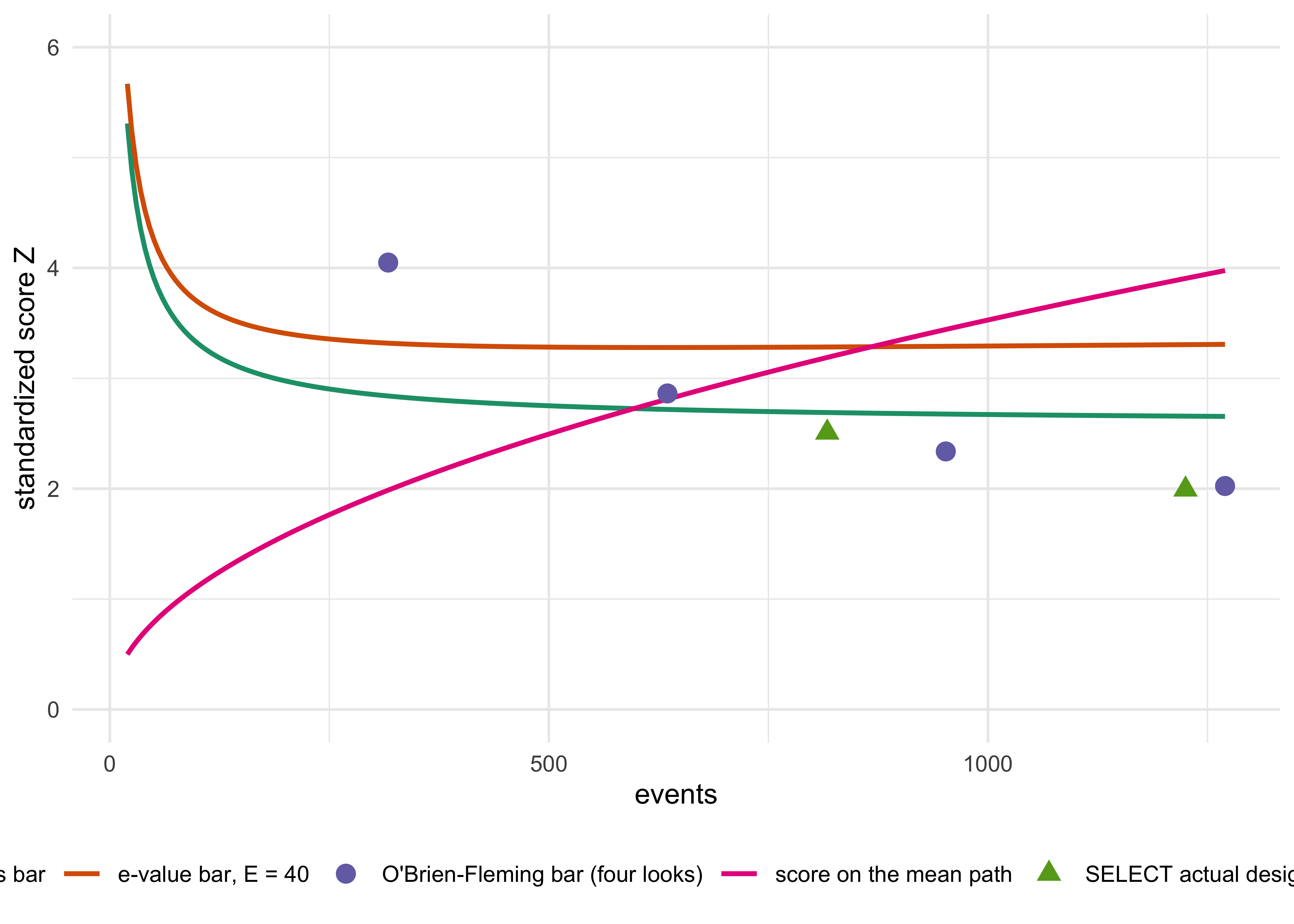
The figure also shows why the conditional medians in the table are not the mean-path crossings (about 600 events for the Bayesian bar and 870 for the e-value bar, mean-path approximations and not stopping times): a rule that can act at any moment stops early on the paths where noise has helped, and the median over paths that succeed sits below the crossing of the average path. The group sequential rules have far fewer moments at which noise can help them.
The ordering of the Bayesian and e-value rules is robust to the prior scale. Over \(\tau \in \{0.15, 0.25, 0.40, 0.60\}\), whose prior intervals for the hazard ratio run from tight to very loose, the calibrated Bayesian rule stops earlier than the e-value rule, on both the conditional and the all-trial scale (Table 21.2):
taus <- c(0.15, 0.25, 0.40, 0.60)
sens <- do.call(rbind, lapply(taus, function(tau) {
  r <- select_simulate(d_tot, HR, nsim = 20000, tau = tau, seed = 5000 + round(100 * tau))$rows
  data.frame(tau = tau, prior_HR = sprintf("%.2f to %.2f", exp(-1.96 * tau), exp(1.96 * tau)),
             bs = r$median_events_success[3], ba = r$median_events_all[3], pb = r$power[3],
             es = r$median_events_success[2], ea = r$median_events_all[2], pe = r$power[2])
}))
knitr::kable(data.frame(sens$tau, sens$prior_HR, sprintf("%.0f / %.0f (%.1f%%)", sens$bs, sens$ba, 100 * sens$pb),
                        sprintf("%.0f / %.0f (%.1f%%)", sens$es, sens$ea, 100 * sens$pe)),
col.names = c("tau", "prior 95% HR interval", "Bayes conditional / all-trial median (power)", "e-value conditional / all-trial median (power)"), align = "rlrr")| tau | prior 95% HR interval | Bayes conditional / all-trial median (power) | e-value conditional / all-trial median (power) |
|---|---|---|---|
| 0.15 | 0.75 to 1.34 | 494 / 510 (95.4%) | 674 / 762 (83.1%) |
| 0.25 | 0.61 to 1.63 | 476 / 502 (93.9%) | 612 / 710 (82.9%) |
| 0.40 | 0.46 to 2.19 | 462 / 494 (93.1%) | 594 / 715 (81.0%) |
| 0.60 | 0.31 to 3.24 | 466 / 506 (92.5%) | 618 / 766 (78.1%) |
In our run the Bayesian conditional median ranges from 462 to 494 events and the all-trial median from 494 to 510, and the e-value conditional median from 594 to 674 and its all-trial median from 710 to 766, with power as shown. The ranges differ slightly from those in the working paper, which are for a different random stream; the ordering does not. All of it is conditional on a hazard ratio held at 0.80, which is the point estimate of a trial that succeeded. The point estimate of a trial that succeeded is on average somewhat optimistic, so a trial run at the true effect would, to that extent, need more events than these medians, and this reconstruction is not a power calculation made before the trial. It is a description of what each rule needs to see if the world is as the trial found it.
From here to the end of the chapter every conversion of events into time, exposure, QALYs or money is a modeled counterfactual: it combines the simulated stopping distribution with an accrual model and with assumptions about what would have happened to patients after a decision. Translating events into calendar time needs an accrual model. We take enrollment linear over 36 months, the trial running to 60 months, and events accruing in proportion to cumulative person time, which reproduces a mean follow-up of 42 months against the reported 39.8.
m <- select_month_of_events(c(Bayes = mda_b, `e-value` = mda_e, `O'Brien-Fleming` = mda_o, `SELECT actual` = mda_a), d_tot)
m_b <- m[["Bayes"]]
The all-trial median decision points fall at month 34 for the Bayesian rule, month 41.6 for the e-value rule, month 49.5 for the four-look group sequential design and month 45 for SELECT’s actual design, against a read-out at month 60. The Bayesian median falls about 8 months before the e-value median, 15 months before the four-look design’s, 11 months before SELECT’s actual design’s, and 2.2 years before the trial’s read-out.
The quantity that matters clinically is exposure. Total exposure in SELECT was about 58,400 patient-years (enrollment times the reported mean follow-up of 39.8 months), of which about 29,200 were on placebo. The accounting below (Table 21.9) converts the expected stopping point of the Bayesian rule, averaged over all simulated trials with the trials that never cross counted at their maximum, into the placebo patient-years and placebo events that would come after it. Three assumptions carry it: events are uniform in person time, placebo participants would have been offered active treatment at the decision so that the events they would otherwise have had are prevented at the trial’s observed relative reduction, and the decision would have been acted on. The figures are an order of magnitude and not a count. For REWIND the median follow-up of 5.4 years stands in for the mean, and the two are not the same.
The medians in Table 21.1 are a summary. The question a DMC faces is concrete: at this look, with these data, does the rule permit a recommendation? Table 21.3 answers it on the mean path at the four looks a group sequential design would have scheduled.
lt <- select_look_table(d_tot, HR)
yn <- function(b) ifelse(b, "yes", "no")
tab <- data.frame(events = lt$events, Z = sprintf("%.2f", lt$z), `OBF bar` = sprintf("%.2f", lt$obf_bound), `OBF stops` = yn(lt$z >= lt$obf_bound),
                  `log E` = sprintf("%.2f", lt$log_bf), `e-value stops` = yn(lt$log_bf >= log(40)),
                  `Pr(benefit)` = sprintf("%.4f", lt$post_prob), `Bayes stops` = yn(lt$post_prob >= res$pstar), check.names = FALSE)
knitr::kable(tab, align = "rrrcrcrc")| events | Z | OBF bar | OBF stops | log E | e-value stops | Pr(benefit) | Bayes stops |
|---|---|---|---|---|---|---|---|
| 318 | 1.99 | 4.05 | no | 0.75 | no | 0.9651 | no |
| 635 | 2.81 | 2.86 | no | 2.40 | no | 0.9963 | yes |
| 952 | 3.44 | 2.34 | yes | 4.17 | yes | 0.9996 | yes |
| 1270 | 3.98 | 2.02 | yes | 6.01 | yes | 0.9999 | yes |
Two readings of the table should be separated. At the first interim, the group sequential committee is shown a standardized score of 1.99 against a boundary of 4.05 and must continue. The Bayesian committee is shown a posterior probability of benefit of 96.5 percent and must also continue, since its calibrated threshold is 99.5 percent. The two agree. At the second interim they part. The score is 2.81 against a boundary of 2.86, so the four-look design continues by a margin of 0.05; the e-value stands at \(\log E = 2.4\) against the 3.69 it needs; and the posterior probability of benefit is 99.63 percent, which clears the calibrated threshold, so the Bayesian rule stops. On the mean path, the four-look design stops at the third look, another 317 events after the Bayesian decision at the second look.
The near miss at the second look is a reminder of how much turns on the spacing of looks, which a group sequential design fixes in advance. The calibrated Bayesian rule may act at any count on its prespecified monitoring grid, within the 1,270-event horizon. It is also a reminder of why a mean path is not a trial: a single real path would sit above or below 2.81 at that look, and the four-look rule would have stopped on a substantial fraction of paths there. SELECT’s actual interim, at 817 events, would show a mean-path score of 3.19 against a boundary of 2.51, but the trial’s actual interim came at 831 events, where the efficacy boundary was crossed and the data monitoring committee recommended continuing (FDA clinical review of NDA 215256 s011, pp. 65-66). Crossing is necessary but not sufficient for stopping, which is one more reason to read the reconstruction through the all-trial table and not through the mean path.
The e-value rule uses the same normal prior scale \(\tau\) and the same score \(S\) as the Bayesian rule, with \(I_n = d/4\) events-based information and \(A = I_n + 1/\tau^2\). The simulated Bayesian rule acts when \(\Pr(\theta > 0 \mid \text{data}) = \Phi(S/\sqrt{A}) \ge p^\ast\), which on the scale \(Z = S/\sqrt{I_n}\) is \(Z \ge \sqrt{1 + 1/(I_n\tau^2)}\, z_{p^\ast}\) with \(z_{p^\ast} = \Phi^{-1}(p^\ast)\), or \(Z^2 \ge (1 + 1/(I_n\tau^2))\, z_{p^\ast}^2\) with \(Z > 0\). The e-value rule acts when the mixture likelihood ratio \(E_n\) reaches \(1/\alpha\), which on the same scale is \(Z^2 \ge (1 + 1/(I_n\tau^2))\,[\log(1 + I_n\tau^2) + 2\log(1/\alpha)]\) with \(Z > 0\). At \(\tau = 0.25\) and \(p^\ast = 0.9952\) the Bayes bar is \(Z^2 \ge 7.6\) at 464 events and 7.0 at 1,270, and the e-value bar is 10.8 and 10.9, so the e-value rule asks for 3.2 more units of \(Z^2\) at 464 events and 3.9 more at 1,270. The constant \(2\log(1/\alpha) = 7.38\) at \(\alpha = 0.025\) is, for this normal-mixture construction and in the large-information approximation, the surcharge of the e-value bar over the uncalibrated Bayes-factor rule at posterior odds 1, \(Z^2 \ge \log(1 + I_n\tau^2)\), of Chapter 11 and Chapter 12; the exact surcharge is \(7.38\,(1 + 1/(I_n\tau^2))\). It is not a universal cost of anytime validity, since other e-processes behave differently. It is also not the surcharge over the calibrated posterior-probability rule simulated here, whose bar \(p^\ast\) was itself raised by simulation to pay for monitoring on the grid. The e-value rule’s realized type I error of about 0.6 percent against a budget of 2.5 percent is the visible form of the remaining difference: it is paying for protection at stopping times this trial never used. In this construction the surcharge is a constant in the large-information approximation, and its relative cost falls only as \(1/\log I_n\); see Chapter 12.
The reconstruction is only useful if the Bayesian rule could have been proposed, accepted and run. Walk through the four principles of the FDA adaptive-designs guidance (U.S. Food and Drug Administration 2019a) and the success-criterion language of the Bayesian draft (U.S. Food and Drug Administration 2026b).
Error control. This is met by construction in the reconstruction, on the event grid and to the 1,270-event horizon, because \(p^\ast\) was found by simulation so that the one-sided familywise type I error under the monitoring plan is 2.5 percent. That fixes the rejection proportion in the calibration sample, not the population error, so a protocol would report the Monte Carlo uncertainty (about 0.0008 at 40,000 paths), validate the threshold on independent null simulations as above, and repeat both across nuisance scenarios. The draft describes calibration as one of three routes, and for a design with a frequentist analysis plan and no borrowing it is the usual one. The weakness is that the calibration holds under a specific monitoring plan. A rule calibrated to a fine grid is conservative for a DMC that meets twice a year, because any subset of the grid inherits the bound. A rule calibrated to meetings twice a year is anti-conservative if the committee also looks ad hoc, for example after a safety signal. A DMC that cannot commit to a schedule can calibrate to a dense grid at the cost of a higher threshold, but monitoring off the grid or beyond the horizon needs recalibration, and a trial that cannot bound its looks should use a fixed design, a spending function or an anytime-valid rule.
Reliable estimation. A trial that stops at the conditional median of 464 events yields a hazard ratio estimate that is biased away from the null on average, as is true of trials that stop early for efficacy, and the confidence interval is wider than the interval from 1,270 events by about \(\sqrt{1270/464} = 1.65\). The Bayesian posterior shrinks the estimate towards the prior, which is a correction in the right direction but not a free one. The trial’s other jobs would also suffer: the key secondary endpoints, the safety database for an agent intended for long-term use, and the subgroup results a label depends on all need events and patient-years, not just a primary endpoint that crossed a bar. For a drug intended for chronic use by people without diabetes, a regulator may well prefer the longer exposure. This is a real cost and the reason the calendar saving in this chapter should not be read as a recommendation.
Prespecification. The prior scale, the threshold, the monitoring schedule and the stopping rule would all have to be written into the protocol and the statistical analysis plan, prospectively. E9 requires interim analyses to be planned and described in the protocol (Section 4.5) and permits justified amendments before unblinded access to comparative data, with their statistical consequences addressed (International Council for Harmonisation 1998). The simulation report that supports them is the operating-characteristics evidence the FDA asks for (Chapter 14).
Trial integrity. The DMC would have been shown a posterior probability and a threshold instead of a boundary. The sponsor would remain blind to the interim comparisons, as it does under a group sequential plan. Nothing about the Bayesian rule changes the firewall; what changes is the number the committee reads.
The regulator’s question about the prior is the one a group sequential design never faces. Here it is answered the way the draft asks: the prior is skeptical, it is prespecified, and its influence on the decision is bounded by the calibration, since a different \(\tau\) changes \(p^\ast\) and leaves the simulated type I error unchanged (see Chapter 8). A regulator who accepts that the final decision rule is “reject when the calibrated posterior probability exceeds \(p^\ast\)” is accepting a test with simulated size and power, which is also what it accepts from an O’Brien-Fleming design. In the language of the substantial-evidence draft (U.S. Food and Drug Administration 2026a), the evidence in either case is a single well-controlled trial whose persuasiveness comes from its effect size and its error control, and a hazard ratio of 0.80 with a final score near 4 is persuasive under any of the rules.
REWIND randomized 9,901 patients with type 2 diabetes to weekly dulaglutide or placebo, enrolling from August 2011 to August 2013 with a median follow-up of 5.4 years, and reported in 2019 (Gerstein et al. 2019). The primary composite cardiovascular outcome occurred in 594 of 4,949 on dulaglutide and 663 of 4,952 on placebo, so 1,257 events, with a hazard ratio of 0.88, a 95 percent interval from 0.79 to 0.99, and \(p = 0.026\).
REWIND ran in the regulatory setting of the 2008 diabetes guidance (U.S. Food and Drug Administration 2008), which asked sponsors of new glucose-lowering drugs to show that the drug did not raise cardiovascular risk beyond a prespecified margin on the hazard ratio. That is the historical context, but REWIND itself was designed to demonstrate cardiovascular superiority, with 90 percent power, and not merely to exclude the 2008 margin (Gerstein et al. 2019). A reconstruction that asks about stopping for benefit is therefore as natural for REWIND as for SELECT, and the contrast below is about the size of the effect and not about the purpose of the trial.
The information content is almost identical to SELECT, 1,257 events against 1,270. The effect is half the size on the log scale, 0.128 against 0.223, so the final standardized score implied by the rounded hazard ratio is 2.27 rather than 3.98 (2.23 is implied by the published two-sided \(p\) value of 0.026; the gap is rounding in the hazard ratio). This is a trial that barely cleared its threshold, and it is exactly the case in which the advantages of continuous monitoring should be expected to shrink.
res_rw <- select_simulate(d_tot = 1257, HR = 0.88, nsim = 40000, seed = 2011)
o <- order(-res_rw$rows$median_events_all[1:3])
ti <- c(res_rw$gs_typeI, res_rw$ev_typeI, res_rw$bayes_typeI)[o]
tab <- res_rw$rows[1:3, ][o, ]
tab <- data.frame(rule = tab$rule, `median events, trials that declare efficacy` = round(tab$median_events_success),
                  `median events, all trials` = round(tab$median_events_all), `mean events, all trials` = round(tab$mean_events_all),
                  power = sprintf("%.1f%%", 100 * tab$power), `type I error` = sprintf("%.2f%%", 100 * ti), check.names = FALSE)
tab <- rbind(tab, data.frame(rule = "The trial as conducted", `median events, trials that declare efficacy` = 1257, `median events, all trials` = 1257,
                             `mean events, all trials` = NA, power = NA, `type I error` = NA, check.names = FALSE))
options(knitr.kable.NA = "")
knitr::kable(tab, align = "lrrrrr", row.names = FALSE)| rule | median events, trials that declare efficacy | median events, all trials | mean events, all trials | power | type I error |
|---|---|---|---|---|---|
| O’Brien-Fleming, four scheduled looks, alpha = 0.025 | 942 | 1257 | 1112 | 60.7% | 2.57% |
| E-value mixture, continuous, E >= 40 | 766 | 1257 | 1123 | 25.7% | 0.60% |
| Bayes posterior, continuous, p* = 0.995 | 680 | 1257 | 973 | 49.1% | 2.50% |
| The trial as conducted | 1257 | 1257 |
Three things change from SELECT, and all three come from the weaker effect.
The speed advantage shrinks, and the conditioning matters more. Among trials that declare efficacy the Bayesian rule acts at a median of about 680 events, 54 percent of the trial’s total, against 37 percent in SELECT. But it declares efficacy in only 49 percent of the trials, so over all trials the median ending point is the maximum, 1,257 events, and the mean is 973 (77 percent of the total, against 44 percent in SELECT). A conditional median here describes only the trials that happened to succeed. A weaker effect takes longer to establish at any bar, and the relative gain from lowering the bar falls accordingly.
Power falls for every rule and the gap between the rules widens. In SELECT the calibrated Bayesian rule had power of 94.7 percent against 97.7 percent for the four-look design; here the four-look design again has the highest power, about 60.7 percent against the Bayesian rule’s roughly 49 percent. A design that concentrates its error budget at the final analysis is better placed to detect an effect that only ever reaches \(Z = 2.27\) than a rule that must hold its level against monitoring on a fine grid.
The e-value rule fails outright. Its power is about 26 percent, so about 74 percent of the time it would not have reached its bar by the end of a trial of this size at this effect. Its realized type I error is about 0.6 percent against a budget of 2.5. This is the surcharge at its most damaging: on the mean path the trial’s total evidence is \(Z^2 = 5.1\), against an exact e-value bar at 1,257 events of 10.9, of which the large-information approximation of the surcharge over the uncalibrated Bayes-factor bar is 7.38 (the exact surcharge is \(7.38(1 + 1/q)\), about 7.8 at \(q = 19.6\)). A bar that high cannot be met on the mean path. Sokolova and Sokolov report the same phenomenon in a mortality trial with a small absolute effect, where the e-value rule needed several times the patients the trial enrolled (Sokolova and Sokolov 2026).
lt_rw <- select_look_table(1257, 0.88)
knitr::kable(round(lt_rw, 3), row.names = FALSE, align = "r")| events | z | obf_bound | log_bf | post_prob |
|---|---|---|---|---|
| 314 | 1.133 | 4.049 | -0.355 | 0.849 |
| 628 | 1.602 | 2.863 | -0.026 | 0.937 |
| 943 | 1.963 | 2.337 | 0.426 | 0.971 |
| 1257 | 2.266 | 2.024 | 0.930 | 0.986 |
The look-by-look table (Table 21.5) tells the same story as the medians. On the mean path the four-look design does not stop at the first three looks and crosses at the last, where the score is 2.27 against a bar of 2.02. The Bayesian posterior probability of benefit reaches 0.986 at the end, and the calibrated threshold of 0.995 is not reached on the mean path at any of the four looks. The Bayesian rule that stops at a conditional median of 680 events does so on the paths where chance has helped, and fails to stop on about 51 percent of paths.
The honest conclusion for REWIND is that the scheduled design was the right choice, and a Bayesian statistician advising the sponsor would have said so if the expected effect was a hazard ratio near 0.88. Four things follow for a protocol.
First, the reconstruction does not rescue the argument for continuous monitoring in a marginal trial, and it should not be offered to a regulator as if it did. The regulator’s concern with a glucose-lowering drug would also include the one stated in the 2008 guidance: precision at the upper bound of the interval, which is a property of the full trial and cannot be got from half of it.
Second, the same Bayesian machinery is useful for a different purpose in such a trial. A posterior distribution for the hazard ratio from the final data, with a skeptical prior, answers the question the 2008 guidance asks (is the upper bound of the effect on cardiovascular risk below the margin?) in the units of the margin. This does not change when the trial can stop; it changes how the result is reported (Chapter 6 and Chapter 7).
Third, the contrast between SELECT and REWIND is itself the finding. The saving from continuous Bayesian monitoring grows with the size of the effect relative to the precision, which a sponsor knows only roughly in advance. The assurance calculation of Chapter 9 is the tool for deciding which design to pick before the trial: the average of the probability of success over a prior on the effect. A prior that puts most of its mass on hazard ratios near 0.80 favors continuous monitoring; a prior centered at 0.90 does not.
Fourth, the reconstruction conditions on the observed effect. For REWIND this is a hazard ratio of 0.88 that barely cleared the bar. Had the true effect been closer to 0.90 the trial would more likely have failed, and the reconstruction would show fewer simulated trials declaring efficacy at a true hazard ratio of 0.90. Assessing early futility would require an additional prespecified rule and a separate operating-characteristics calculation (Chapter 15).
The reconstruction asks when a decision could have been taken. A separate question is what the final data say, and there the normal approximation is enough. The log hazard ratio is estimated at \(\log 0.88 = -0.128\) with a standard error of about 0.058, read from the published interval. Table 21.6 gives the posterior under a flat prior and under three skeptical priors centered on no effect, with prior standard deviations of 0.2, 0.1 and 0.05 on the log hazard ratio (a standard deviation of 0.05 says that a hazard ratio below 0.90 or above 1.11 is a two-standard-deviation event before the trial).
se_rw <- (log(0.99) - log(0.79)) / (2 * qnorm(0.975))
sds <- c(Inf, 0.2, 0.1, 0.05)
rw_pr <- do.call(rbind, lapply(sds, function(s0) {
  r <- reanalysis_normal(-log(0.88), se_rw, 0, s0, mcid = -log(0.9))
  data.frame(prior = if (is.finite(s0)) sprintf("N(0, %s^2)", format(s0)) else "flat",
             hr = exp(-r$post_mean), lo = exp(-r$post_mean - 1.96 * r$post_sd), hi = exp(-r$post_mean + 1.96 * r$post_sd),
             p1 = r$p_benefit, p9 = r[[4]])
}))
knitr::kable(data.frame(`prior on log HR` = rw_pr$prior, `posterior HR` = sprintf("%.3f", rw_pr$hr),
                        `95% interval` = sprintf("%.2f to %.2f", rw_pr$lo, rw_pr$hi),
                        `Pr(HR < 1)` = sprintf("%.3f", rw_pr$p1), `Pr(HR < 0.9)` = sprintf("%.2f", rw_pr$p9), check.names = FALSE),
align = "lrrrr", row.names = FALSE)| prior on log HR | posterior HR | 95% interval | Pr(HR < 1) | Pr(HR < 0.9) |
|---|---|---|---|---|
| flat | 0.880 | 0.79 to 0.99 | 0.987 | 0.65 |
| N(0, 0.2^2) | 0.889 | 0.80 to 0.99 | 0.984 | 0.59 |
| N(0, 0.1^2) | 0.908 | 0.82 to 1.00 | 0.973 | 0.43 |
| N(0, 0.05^2) | 0.947 | 0.88 to 1.02 | 0.927 | 0.09 |
The direction of the effect is robust to any reasonable skepticism, and its size is not. A clinician asking whether dulaglutide lowers cardiovascular risk can be fairly confident that it does (the probability is 0.93 even under the strictest prior). A payer asking whether it lowers risk by 10 percent or more should be much less confident: that probability falls from 0.65 under a flat prior to 0.09 under the strictest, and the answer depends on how skeptical the payer’s prior is. This is the same lesson as the reconstruction, seen from the end of the trial.
The preceding two cases compared a drug with placebo. SURPASS-CVOT compared two active drugs, which changes the question (Nicholls et al. 2025). It randomized 13,299 adults with type 2 diabetes and established atherosclerotic cardiovascular disease, double blind and 1:1, to weekly tirzepatide (up to 15 mg) or dulaglutide 1.5 mg, the dose that REWIND had shown to reduce cardiovascular events. After 134 exclusions for ineligibility the modified intention-to-treat population was 13,165 (6,586 on tirzepatide and 6,579 on dulaglutide). The primary outcome was the first of cardiovascular death, myocardial infarction or stroke, and the primary hypothesis was noninferiority: the upper limit of the 95.3 percent confidence interval for the hazard ratio had to lie below 1.05, and superiority could be claimed if the upper limit was below 1.00. The traditional logic of the noninferiority test, a margin fixed in advance and a one-sided bound on the interval, is the one set out in Chapter 4.
The primary outcome occurred in 801 patients (12.2 percent) on tirzepatide and 862 (13.1 percent) on dulaglutide, a hazard ratio of 0.92 with a 95.3 percent confidence interval from 0.83 to 1.01. Noninferiority was established (\(p = 0.003\)) and superiority was not (\(p = 0.09\)). We omit the secondary and component hazard ratios, which we have not checked against the full report.
z_s <- qnorm(1 - 0.047 / 2)
se_s <- (log(1.01) - log(0.83)) / (2 * z_s)
r_s <- reanalysis_normal(-log(0.92), se_s, 0, Inf, mcid = c(-log(1.05), -log(0.9)))
p_ni <- r_s[[4]]; p_sup <- r_s$p_benefit; p_90 <- r_s[[5]]
se_c <- sqrt(se_s^2 + se_rw^2); hr_c <- 0.92 * 0.88
ci_c <- exp(log(hr_c) + c(-1, 1) * 1.96 * se_c)
tab <- data.frame(quantity = c("Pr(HR < 1.05), noninferiority", "Pr(HR < 1), superiority", "Pr(HR < 0.9), a reduction of 10% or more",
                               "Indirect HR against placebo (95% interval)"),
                  value = c(sprintf("%.3f", p_ni), sprintf("%.3f", p_sup), sprintf("%.2f", p_90),
                            sprintf("%.2f (%.2f to %.2f)", hr_c, ci_c[1], ci_c[2])))
knitr::kable(tab, align = "lr", row.names = FALSE)| quantity | value |
|---|---|
| Pr(HR < 1.05), noninferiority | 0.996 |
| Pr(HR < 1), superiority | 0.954 |
| Pr(HR < 0.9), a reduction of 10% or more | 0.33 |
| Indirect HR against placebo (95% interval) | 0.81 (0.70 to 0.94) |
The Bayesian reading (Table 21.7) answers the questions a prescriber asks, and it does so on a continuous scale. The posterior probability that tirzepatide is noninferior, that is, that the hazard ratio is below 1.05, is 0.996, and the probability that it is superior is 0.954. The trial “failed” to show superiority because the upper limit of 1.01 sat just above 1.00, yet the probability that the hazard ratio is below one is 0.95. These are not competing statements: the frequentist \(p = 0.09\) is the chance, if the hazard ratio were exactly one, of data at least this extreme in either direction, and the posterior probability is a statement about the hazard ratio given the data and a flat prior. Neither is wrong, and a decision-maker needs the second to weigh a benefit against a cost. The probability of a reduction of at least 10 percent is only 0.33, which is the honest size of the uncertainty about how much better tirzepatide is. As with REWIND, the posterior under a skeptical prior would be pulled toward one, and for a trial of this size the flat-prior numbers are the upper end of what the data support.
Tirzepatide was never tested against placebo for cardiovascular outcomes in this trial, and the missing comparison can be filled by an indirect chain through dulaglutide, shown in the last row of Table 21.7 (0.81, interval 0.70 to 0.94). The assumption of transportability from REWIND is the whole of the argument, and it is exactly what a Bayesian borrowing model makes explicit and discounts. The calculation, the discounted versions and the comparison with the published indirect analysis of Sattar et al. (2026) are in Section 19.12; the clinical point is that two numbers for the same question differ in what they adjust for, and an indirect comparison rests on its assumptions.
For Bayesian reanalyses of other landmark trials, with the priors and the arithmetic laid out, see Chapter 22.
TRAILBLAZER-ALZ 2 randomized 1,736 participants with early symptomatic Alzheimer’s disease to donanemab or placebo, with efficacy measured at 18 months (76 weeks), and reported a 35 percent slowing of decline on its integrated Alzheimer’s Disease Rating Scale (iADRS) in the prespecified low and medium tau population of 1,182 participants, and a 22 percent slowing in the combined population of 1,736 (Sims et al. 2023). The primary analysis was prespecified for two populations, the tau-defined one and the combined one, and the trial therefore had to choose how to spend its type I error between them. The order of testing is given in the publication and its supplement (Sims et al. 2023).
This is a traditional design in the sense of this book: a fixed duration, a prespecified primary analysis with a multiplicity procedure across populations, and a single final analysis. It differs from a textbook parallel-group trial in two respects. Both are prespecified design features, and neither is Bayesian as conducted; a Bayesian analysis could be proposed for the second.
The first is that treatment duration was guided by a biomarker. Participants completed their course of donanemab once they reached a prespecified level of amyloid plaque clearance, and the report gives 52 percent of the low and medium tau participants as having reached the clearance criterion by one year, among those with a PET assessment at that visit (Sims et al. 2023). This is a stopping rule applied to each participant rather than to the trial, driven by an intermediate biomarker. It is a prespecified biomarker-guided treatment strategy, and it does not require Bayesian inference. It is related to individualized dosing in the patient-specific dose-finding designs reviewed in Chapter 17, and because it depends only on each participant’s own biomarker and not on accumulating comparative results, it is a treatment strategy and not a trial adaptation in the sense of the FDA guidance. It is also a rule that a fixed-duration comparison cannot evaluate on its own: the trial estimates the effect of the strategy “stop when cleared” against placebo, not the effect of a fixed dose and duration, and the estimand has to say so (ICH E9(R1), Chapter 5).
The second is baseline tau stratification. The trial reports a 35 percent effect in one stratum and a 22 percent effect in the combined population. Tau status is measured at baseline, and the strata do not change in response to accumulating results, so this is baseline stratification and not an adaptive feature. The standard apparatus requires that the populations and the order of testing be designated before the data arrive, and the designation then governs the claim. A prespecified hierarchical model (Chapter 19, Chapter 10) could estimate effects in both disjoint strata with borrowing between them. Population claims and their success criteria would still require prespecification and an evaluation of false-positive risks. The sizes of the two strata, 1,182 participants in the low and medium tau stratum and 552 in the high tau stratum as reported, do not by themselves establish that borrowing would be large; that depends on the between-stratum variance, as the illustration below shows.
The arithmetic of that shrinkage is simple enough to show. Suppose the two strata have estimated effects with standard errors proportional to \(1/\sqrt{n}\), and the between-stratum standard deviation \(\tau_b\) of the true effect is the quantity the data cannot tell us much about. The weight on the stratum’s own estimate is \(\tau_b^2/(\tau_b^2 + s^2)\), where \(s\) is its standard error and \(\tau_b\) is the between-stratum standard deviation. The smaller the stratum and the smaller the between-stratum variance, the more the estimate is pulled to the pooled one.
# Illustration only: two strata with effect estimates on a common scale, standard errors scaling as 1/sqrt(n).
# These are NOT the trial's estimates; they show how the shrinkage weight depends on stratum size and tau.
n <- c(1182, 552)
s <- 10 / sqrt(n)                  # arbitrary common scale, so the weights are what matter
tau_b <- c(0.1, 0.2, 0.4)           # between-stratum sd, same scale
W <- t(sapply(tau_b, function(t) t^2 / (t^2 + s^2)))
knitr::kable(data.frame(tau_b, W), digits = 2, align = "rrr",
col.names = c("Between-stratum sd", "Weight, large stratum", "Weight, small stratum"))| Between-stratum sd | Weight, large stratum | Weight, small stratum |
|---|---|---|
| 0.1 | 0.11 | 0.05 |
| 0.2 | 0.32 | 0.18 |
| 0.4 | 0.65 | 0.47 |
The numbers in Table 21.8 are illustrative and not the trial’s, which we do not have in the form the calculation needs.
Which analysis a regulator prefers is not a question we can settle. The trial as conducted had to choose a primary population and a multiplicity procedure, and it did, in a way the FDA could review against the substantial-evidence standard. A hierarchical Bayesian analysis of the two strata would be a proposed alternative, not a description of what the trial did, and would need three things the draft guidance asks of any borrowing: a prespecified model, a stated rationale for exchangeability of the strata, and a simulation of its type I error across the scenarios in which the effect is present in one stratum only (Chapter 19). Those scenarios are the ones that matter, because a hierarchical model that shrinks a null stratum towards a positive pooled effect will raise the false-positive rate for that stratum. The regulatory cost is a longer simulation report and a more demanding conversation about the prior on the between-stratum variance.
For the biomarker-guided duration, the regulator’s concern is the estimand and the integrity of blinding (the blind has to survive the switch when a participant stops active treatment after clearance, which is a matter of masking procedure and not of the analysis). Neither is Bayesian or frequentist. They are the design properties that made a prespecified biomarker-guided feature acceptable to the FDA in this case.
The lesson is different from SELECT’s. In SELECT, a Bayesian monitoring rule would change when the trial stops. In TRAILBLAZER-ALZ 2, the traditional apparatus handled two prespecified features, and the trial shows that regulators accept them when they are specified in advance. A hierarchical Bayesian analysis of the strata would not make the trial more or less adaptive. It would express the stratum analysis through one model in place of a testing hierarchy, at the price of the prespecification and simulation described above.
The phase 2/3 trial of the BNT162b2 mRNA vaccine (Protocol C4591001, Pfizer and BioNTech) began in July 2020 and reported the efficacy of the vaccine in preventing COVID-19 (Polack et al. 2020). Its statistical analysis plan, posted on ClinicalTrials.gov, makes the primary analysis Bayesian (Pfizer Inc. 2022). This case differs from the other four in kind: the Bayesian rule is not a counterfactual reconstruction but the decision rule the trial itself used, and it supported a regulatory action. The beta-binomial model of Chapter 6 is the whole of the machinery.
The conjugate beta-binomial model, with prior Beta(0.700102, 1) on the vaccine share of cases, the transformation to VE and the posterior arithmetic, is worked in full in Section 6.12. The plan calls the prior minimally informative and says it can be considered pessimistic. The case-specific points are the success criterion, \(\Pr(\mathrm{VE} \ge 30\% \mid \text{data})\), which must exceed 0.995 at an interim analysis and 0.986 at the final analysis, with the thresholds calibrated so that the overall one-sided type I error is 2.5 percent (Section 7.1 of the plan; the calibration is the kind of simulation of Chapter 14). Two primary objectives, VE in participants with no evidence of prior infection and VE in all participants, were evaluated in sequence. The final analysis was planned at 164 first primary cases, with interim looks and a futility rule based on the predictive probability of success, nonbinding, of 5 percent or less.
Two features set it apart from SELECT’s reconstruction. The bar is on VE of 30 percent, a margin of clinical relevance, and not on zero, so the criterion is the \(\Pr(\delta > a \mid \text{data}) > c\) of the FDA draft with \(a\) different from zero. And the model is conjugate, so each look is a closed-form calculation with no simulation of the posterior itself, only of the operating characteristics.
a0 <- 0.700102; pi30 <- 0.7 / 1.7              # VE = 30% corresponds to pi_v = 0.7/1.7
pr_ve30 <- function(v, p) pbeta(pi30, a0 + v, 1 + p)   # v vaccine cases, p placebo cases
th <- qbeta(c(0.975, 0.5, 0.025), a0 + 8, 1 + 162)
ve <- round(100 * (1 - (2.222 / 2.214) * th / (1 - th)), 1) # posterior 2.5%, 50%, 97.5% for VE; surveillance-time ratio 2.222/2.214 (FDA briefing, Table 6)The published analysis counted 8 cases in the vaccine group and 162 in the placebo group, a vaccine efficacy of 95.0 percent with a 95 percent credible interval of 90.3 to 97.6 percent (Polack et al. 2020). Our calculation (Section 6.12), with the surveillance-time ratio of 2.222 to 2.214 reported in the FDA briefing document, gives 90.3 to 97.6 percent against the published 90.3 to 97.6 (the counts of 8 and 162 are exact), and a posterior probability of VE above 30 percent that is indistinguishable from one (1), far above 0.986. FDA issued an emergency use authorization on 11 December 2020 for individuals 16 years of age and older (U.S. Food and Drug Administration 2021a), and approved the biologics license application (Comirnaty) on 23 August 2021, again for those 16 and older (U.S. Food and Drug Administration 2021b).
Where the SELECT and REWIND reconstructions are counterfactuals, BNT162b2 shows the regulatory path already traveled: a minimally informative prior, a margin, calibration to 0.025 one-sided, and a protocol that fixed the thresholds before the first case. One caution. The plan on ClinicalTrials.gov is a sponsor document with several amendments. The efficacy boundaries tabulated in the plan, written as case splits, reproduce from the stated prior: at the final analysis of 164 cases, 53 vaccine cases is the largest count with \(\Pr(\mathrm{VE} > 30\% \mid \text{data}) > 0.986\) (53 gives 0.990, 54 gives 0.985). The backing for a rule of this kind comes from Chapter 6 for the model and Chapter 14 for the calibration.
A claim that a design decides at 486 events (the all-trial median; 464 among trials that declare efficacy) rather than 1,270 is not yet an argument that anyone outside the field will weigh. This section converts it into five currencies. Every conversion is a modeled counterfactual, and the conversions differ in how many assumptions they stack. They use the expected stopping point over all simulated trials, so that trials which never cross, and therefore save nothing, are counted.
These figures are modeled counterfactuals: arithmetic on the trial’s own counts and the simulated all-trial stopping distribution, under the assumptions stated above (events uniform in person time, placebo participants switched at the decision, the decision acted on).
x <- data.frame(trial = c("SELECT", "REWIND"), d_dec = c(mna_b, mna_brw), d_tot = c(1270, 1257),
                n = c(17604, 9901), yrs = c(39.8 / 12, 5.4), ev_placebo = c(701, 663), ev_active = c(569, 594))
x$share <- x$d_dec / x$d_tot                       # expected share of events accrued at the Bayesian decision
x$placebo_py <- (1 - x$share) * x$n * x$yrs / 2    # placebo patient-years afterwards
x$placebo_events <- (1 - x$share) * x$ev_placebo
x$excess <- (1 - x$share) * (x$ev_placebo - x$ev_active)
sel <- x[1, ]; rew <- x[2, ]
knitr::kable(transform(x[, c("trial", "share", "placebo_py", "placebo_events", "excess")], share = round(share, 3),
  placebo_py = round(placebo_py), placebo_events = round(placebo_events), excess = round(excess)), row.names = FALSE,
align = "lrrrr", col.names = c("Trial", "Expected share of events at decision", "Placebo patient-years after", "Placebo events after", "Excess placebo events after"))| Trial | Expected share of events at decision | Placebo patient-years after | Placebo events after | Excess placebo events after |
|---|---|---|---|---|
| SELECT | 0.435 | 16490 | 396 | 75 |
| REWIND | 0.774 | 6037 | 150 | 16 |
Averaged over all simulated trials, the Bayesian rule had accrued 43.5 percent of SELECT’s events when it stopped (a trial that never crosses counted at 1,270), so on average 56.5 percent of the events and of the exposure would have come afterwards. Under the modeled assumptions that is about 16,500 placebo patient-years and 396 of the 701 placebo primary events. The excess over the semaglutide arm is about 75 events: the major adverse cardiovascular events that the treatment would have prevented in a placebo arm switched to treatment at the decision, if the trial’s relative effect held afterwards. This is a model-based expectation and not an observed count. It is also smaller than the figure the conditional median gives (63 percent of events), which describes only the trials that succeed.
Converting to QALYs requires a value per event averted. The composite mixes events worth very different amounts: a nonfatal event in a patient of about sixty carries a utility decrement of roughly 0.05 to 0.12 a year over a remaining life of ten to fifteen years, so of order 0.5 to 1.5 QALYs, while a cardiovascular death averted is worth the discounted remainder of that life, of order six to nine. These are our assumptions, and we report a range and not a figure.
q <- c(1.5, 2, 3)
tab <- sapply(q, function(v) round(x$excess * v)); dimnames(tab) <- list(x$trial, paste(q, "QALY per event"))
knitr::kable(tab, align = "rrr")| 1.5 QALY per event | 2 QALY per event | 3 QALY per event | |
|---|---|---|---|
| SELECT | 112 | 149 | 224 |
| REWIND | 23 | 31 | 47 |
For REWIND, the expected Bayesian stopping point is at about 77 percent of events, so about 6,000 placebo patient-years and 150 of the 663 placebo events come afterwards, of which about 16 are the excess over the dulaglutide arm, under the same assumptions. The modeled in-trial saving is of order a hundred QALYs for SELECT and a small fraction of that for REWIND, not thousands.
Moore and colleagues reviewed the pivotal trials of 59 novel agents approved by the FDA in 2015 and 2016 (Moore et al. 2018). The median estimated cost of a pivotal trial was $19.0 million, the costliest single trial in the review was about $347 million, and the mean estimated cost of the five cardiovascular pivotal trials was $157.2 million (their Table 2). SELECT, with 17,604 patients at 804 sites in 41 countries and about five years of follow-up, is far larger than the typical trial in that review, and we have no published cost for it. We therefore take the cited cardiovascular mean of $157 million as the base case and $350 million and $600 million as scenarios for a larger trial, not as estimates of the cost of any particular trial.
The saving is not proportional to the whole budget. Variable costs, which are site payments, patient visits, monitoring, laboratory work and drug supply, scale with person-time; fixed costs, which are protocol development, startup, regulatory work and the final analysis, do not. With 56.5 percent of the person-time avoided on average, the modeled saving is that share of the variable share.
v <- c(0.5, 0.6, 0.7); tot <- c(157, 350, 600)
tab <- rbind(paste0(round(100 * (1 - sel$share) * v), "%"),
             sapply(v, function(s) paste0("\\$", round((1 - sel$share) * s * tot[1]), " million")),
             sapply(v, function(s) paste0("\\$", round((1 - sel$share) * s * tot[2]), " million")),
             sapply(v, function(s) paste0("\\$", round((1 - sel$share) * s * tot[3]), " million")))
colnames(tab) <- paste0(100 * v, "% variable")
rownames(tab) <- c("saving as a share of total cost", "on a \\$157 million trial", "on a \\$350 million trial", "on a \\$600 million trial")
knitr::kable(tab, align = "rrr")| 50% variable | 60% variable | 70% variable | |
|---|---|---|---|
| saving as a share of total cost | 28% | 34% | 40% |
| on a $157 million trial | $44 million | $53 million | $62 million |
| on a $350 million trial | $99 million | $119 million | $138 million |
| on a $600 million trial | $169 million | $203 million | $237 million |
For a trial of SELECT’s size the order of magnitude is therefore tens to a couple of hundred million dollars, and that is the number a sponsor will find most persuasive. It leaves out the cost of the longer exposure that a regulator might require to build the safety database, which would reduce the saving.
Under the accrual model above, the all-trial median Bayesian decision falls at month 34 against a read-out at month 60, so 26 months or 2.2 years earlier. For REWIND the all-trial median decision is the end of the trial, so there is no median calendar saving, and the expected saving, with the decision at about 77 percent of events on average, is much smaller than SELECT’s, since the Bayesian rule reaches its bar in only about half of the replications.
Multiplying the acceleration by the treated population gives a very large number. We give it, and then explain why it is a bound and not a forecast. Suppose approval moved earlier by 2.2 years (the all-trial median saving) and \(N\) patients received the treatment during that window, at the trial’s placebo event rate of about 2.4 percent a year and its relative reduction of 20 percent.
yrs <- (60 - m_b) / 12
N <- c(1e5, 5e5, 1e6); ev <- N * 0.024 * 0.20 * yrs
knitr::kable(data.frame(`patients treated in the window` = format(N, big.mark = ",", scientific = FALSE),
  `events averted` = format(round(ev), big.mark = ","), `QALYs at 2 per event` = format(round(2 * ev), big.mark = ","), check.names = FALSE),
align = "rrr")| patients treated in the window | events averted | QALYs at 2 per event |
|---|---|---|
| 100,000 | 1,039 | 2,079 |
| 500,000 | 5,196 | 10,393 |
| 1,000,000 | 10,393 | 20,786 |
Two orders of magnitude separate this from the in-trial figures, and that asymmetry is the real economics of trial design: the value of a trial is overwhelmingly in the decision it enables for the population outside it, which is the post-trial population size \(M\) of the loss function in the working paper (Polson and Sokolov 2026). But the calculation assumes that approval, reimbursement, manufacturing and clinical uptake would all have moved forward by the full 2.2 years, and none of those would. Manufacturing capacity for these agents was the binding constraint on access during this period, so the realistic acceleration is a fraction of the statistical one.
The largest sum in the accounting is commercial, and it rests on the least. Patent expiry is fixed, so a cardiovascular indication reached earlier adds the same number of years of protected, label-driven sales. Novo Nordisk reported global Wegovy sales of DKK 58.2 billion for 2024 (Novo Nordisk A/S 2025). The share of sales that the cardiovascular label drives is not public, and we assume 10 to 25 percent. At an assumed 6.9 DKK per dollar the 2024 sales are about $8.4 billion, and brought forward by the all-trial median saving of 2.2 years the label-driven revenue is $1.8 billion to $4.6 billion. This is a modeled counterfactual of revenue, not profit, and an upper bound: approval, reimbursement and uptake would not all have moved forward by the full statistical acceleration, for the reasons given for the population bound above, and the sales level, the label share and the exchange rate are assumptions.
REWIND gives the same arithmetic only conditionally. Trulicity (dulaglutide) had revenue of $4.13 billion in 2019 (Eli Lilly and Company 2022), and the FDA approved its cardiovascular indication on 21 February 2020 (U.S. Food and Drug Administration 2020). In the reconstruction the Bayesian rule acts in only 49 percent of simulated REWIND trials, so the all-trial median saving is zero, because fewer than half of the simulated trials cross. The unconditional expected saving can still be positive: the mean decision falls at 973 of 1,257 events, so on average 23 percent of the events and person time would come after it. The revenue figures below describe the conditional median among trials that cross, and multiplying the crossing probability by a conditional median would not give an expected revenue (that needs the calendar saving averaged over all paths, which the summary output does not keep). Conditional on its acting, the median decision falls at 680 of 1,257 events. Under an accrual model with an assumed 24 months of linear enrollment and the 85 months between the registered start and primary completion dates (ClinicalTrials.gov 2026j), that is month 51, or 2.8 years before the read-out. With an assumed 10 to 20 percent of 2019 sales attributable to the label, the revenue brought forward would be $1.2 billion to $2.3 billion, but only in the trials in which the rule acts, and the scheduled design acts more often there.
Two caveats from the earlier sections apply to every currency in this section. Among trials stopping early for efficacy, naive estimates tend to exaggerate benefit. Skeptical priors may reduce this bias; bias and interval coverage should be evaluated for the specified estimator and stopping rule. And a regulator would want safety follow-up to continue after an efficacy decision, which recovers only part of the cost saving.
| currency | SELECT | basis |
|---|---|---|
| events averted in trial | about 75 | modeled: expected share of events plus a placebo switch assumption |
| placebo patient-years avoided | about 16,500 | modeled: expected share of events plus uniform events in person time |
| QALYs inside the trial | 112 to 224 | plus a QALY value per event |
| calendar time | 26 months before read-out (11 before SELECT’s actual design, at the all-trial medians) | plus an accrual model |
| trial cost | 28 to 40 percent | plus a fixed and variable cost split |
| label revenue brought forward | $1.8 to $4.6 billion of Wegovy revenue | plus a label share, an exchange rate and full acceleration; revenue, not profit |
| population QALYs | thousands | plus an access counterfactual |
Every row is a modeled counterfactual computed from the all-trial distribution of simulated stopping points, and none is an observed fact about the trial. The first two rows rest on the stopping distribution and on assumptions about treatment switching and the uniformity of events. The rest add assumptions we have stated and a reader can vary. We would defend the first two as modeling exercises with few assumptions, the third and fourth as modeling exercises, the fifth as an order of magnitude, the sixth as an upper bound on revenue that rests on an assumed label share, and the seventh only as a bound.
| Traditional (what the trials did) | Bayesian reconstruction | What the regulator will ask | |
|---|---|---|---|
| Monitoring | Event-driven; DMC reviews at scheduled looks, boundaries from a spending function (SELECT: one interim at two thirds of the planned events) | Monitoring of a posterior probability on a fine event grid | The monitoring plan, written in advance (E9 4.5) |
| Decision rule | Test statistic crosses a boundary | \(\Pr(\delta > a \mid \text{data}) > p^\ast\) | Calibration of \(p^\ast\) to 0.025 one-sided by simulation, with Monte Carlo error |
| Type I error | Spent by alpha spending | Calibrated by simulation under the plan | Simulation report, scenarios, Monte Carlo error |
| Prior | None | Skeptical normal on the log hazard ratio | Prespecified, with sensitivity to \(\tau\) |
| Where it wins | Marginal effects, fixed looks (REWIND) | Large effects, DMC that can commit to a plan (SELECT) | Evidence the choice was made before the data |
| What does not change | Randomization, blinding, endpoint, firewall, intention-to-treat estimand | Same | Same |
Where the two agree numerically: with a flat prior, the posterior probability of benefit equals one minus the one-sided \(p\) value, so a single-look Bayesian rule with threshold \(c\) is the fixed one-sided test at level \(1 - c\).
The cases above are trials that have reported. The ones below are running, or have just reported, and each sits next to relevant evidence from a sibling or rival trial. We list them to show where the ideas of this book would apply now, not to predict their results. Design facts are from the ClinicalTrials.gov records (retrieved 10 November 2026, with each record’s last-update date in the references), and the status of a trial is its status on that date; dates marked “est.” are registry estimates and move. We give no result that we could not read in a registry record or a sponsor announcement.
| Trial (drug, sponsor) | Design as registered | Status on 10 November 2026 | What a Bayesian design or analysis would change |
|---|---|---|---|
| PREVAIL (obicetrapib, NewAmsterdam) (ClinicalTrials.gov 2026a) | Randomized, quadruple-masked, placebo-controlled phase 3; 9,541 participants; primary endpoint major adverse cardiovascular events | Active, not recruiting; primary completion est. November 2026 (the record was last updated June 2024) | A discounted prior from the sponsor’s earlier phase 3 trial of the same drug, and an interim decision by the predictive probability of success at completion (Chapter 15) |
| AHEAD 3-45 (lecanemab, Eisai and Biogen) (ClinicalTrials.gov 2026f) | Randomized, quadruple-masked phase 3 in preclinical Alzheimer’s disease; est. 1,400 participants; two primary outcomes, change in the PACC5 composite (A45) and in amyloid PET (A3) at week 216 | Active, not recruiting; primary completion est. December 2028 | The two prevention trials as estimates of a common class effect, so that the first readout updates the second, with biomarker change modeled jointly with cognition |
| TRAILBLAZER-ALZ 3 (donanemab, Lilly) (ClinicalTrials.gov 2026b) | Randomized, double-masked phase 3 in preclinical Alzheimer’s disease; est. 2,996 participants; primary endpoint time to clinical progression on the Clinical Dementia Rating | Active, not recruiting; primary completion est. November 2027 | As above; the endpoints differ (a time to progression and a change score), so exchangeability would have to be argued on a common scale |
| SURMOUNT-MMO (tirzepatide, Lilly) (ClinicalTrials.gov 2026d) | Randomized, double-masked phase 3; 15,374 participants; primary endpoint time to first of all-cause death, nonfatal myocardial infarction, nonfatal stroke, coronary revascularization or heart failure event, up to 5 years | Active, not recruiting; primary completion est. October 2027 | A prior from SELECT and SURPASS-CVOT (Section 21.3), discounted for a five-component composite and a different drug, and calibrated monitoring as in the SELECT reconstruction |
| REDEFINE 3 (CagriSema, Novo Nordisk) (ClinicalTrials.gov 2026i) | Randomized, quadruple-masked phase 3; 7,101 participants aged 55 or older with established cardiovascular disease; primary endpoint time to first 3-point MACE | Active, not recruiting; primary completion est. September 2027 | A power prior for the semaglutide component from SELECT, discounted for the added uncertainty about cagrilintide (Chapter 19) |
| TRIUMPH-3 (retatrutide, Lilly) (ClinicalTrials.gov 2026c) | Randomized, double-masked phase 3, 80 weeks, in obesity with established cardiovascular disease; 1,946 participants in the registry; registered primary outcome percent change in body weight | Completed; topline announced 23 July 2026 (Eli Lilly and Company 2026) | A class prior turns an imprecise cardiovascular interval into a posterior (below) |
| Lp(a)HORIZON (pelacarsen, Novartis) (ClinicalTrials.gov 2026g) | Randomized, double-masked phase 3; 8,323 participants; two primary outcomes, expanded MACE in patients with Lp(a) of at least 70 mg/dL and of at least 90 mg/dL | Completed; Novartis announced on 4 September 2026 that the primary endpoint was not met (Novartis 2026); full results published 7 November 2026 (Cho, Nicholls, et al. 2026) | A posterior for the sizes of benefit the published hazard ratio (1.02, 95 percent interval 0.90 to 1.15) rules out (below) |
| OCEAN(a)-Outcomes (olpasiran, Amgen) (ClinicalTrials.gov 2026h) | Randomized, double-masked phase 3; 7,297 participants; primary endpoint time to coronary heart disease death, myocardial infarction or urgent coronary revascularization | Active, not recruiting; primary completion est. March 2028 | A hierarchical model across the Lp(a) outcomes trials with the depth of Lp(a) lowering as a covariate, and a futility rule on the predictive probability of a clinically meaningful effect |
| ACCLAIM-Lp(a) (lepodisiran, Lilly) (ClinicalTrials.gov 2026e) | Randomized, double-masked phase 3; est. 17,300 participants; primary endpoint time to first MACE-4 | Active, not recruiting; primary completion est. March 2029 | A futility rule and a final sample size set from OCEAN(a) as it reads out |
The traditional designs here are sound for what they are asked to do. All are randomized and masked. Several cardiovascular outcomes trials are event driven; AHEAD and TRIUMPH-3 assess their primary outcomes at specified follow-up times. Each is built to stand alone as substantial evidence, and a sibling trial’s result does not automatically change the analysis plan. Justified amendments based solely on external information may be acceptable while comparative interim results remain protected (U.S. Food and Drug Administration 2019b). For the proposed Bayesian designs, the borrowing and updating procedures, including any incorporation of future sibling results, should be prespecified. The Bayesian changes in the last column are therefore proposals with a price: each borrowed prior must be fixed before the data, discounted and justified, and each design with it simulated for its operating characteristics under a plan the regulator has seen (Chapter 19, Chapter 14). Where we write that a Bayesian rule could stop sooner, the size of the gain depends on an effect size that is not yet known, and the SELECT reconstruction above is not a forecast for any of these trials.
Lilly’s announcement reports 44 five-component events (all-cause death, myocardial infarction, stroke, heart failure event or coronary revascularization) on pooled retatrutide against 52 on placebo, a hazard ratio of 0.82 with a 95 percent interval from 0.55 to 1.22, in prespecified analyses of a trial whose registered primary outcome was weight (Eli Lilly and Company 2026). The three-component MACE hazard ratio in the same announcement was 1.12 (0.64 to 1.96). A frequentist reading of the five-component interval says that benefit is not established, and that is a correct statement about the interval. A Bayesian reading adds what the interval does not say, and shows how much of it depends on the prior. The interval gives the log hazard ratio \(\log 0.82\) with standard error \((\log 1.22 - \log 0.55)/3.92\). For a class prior we use SELECT, with a hazard ratio of 0.80 and interval 0.72 to 0.90 (Lincoff et al. 2023), discounted by inflating its variance (doubling it for half weight, quadrupling it for quarter weight), and for contrast a skeptical normal prior with standard deviation 0.15 and a flat prior (Section 22.1).
est <- log(0.82); se_t <- (log(1.22) - log(0.55)) / 3.92
se_s <- (log(0.90) - log(0.72)) / 3.92
pri <- list(`Flat` = c(0, Inf), `SELECT, half weight` = c(log(0.80), sqrt(2) * se_s),
            `SELECT, quarter weight` = c(log(0.80), 2 * se_s), `Skeptical, N(0, 0.15^2)` = c(0, 0.15))
tri <- t(sapply(pri, function(p) {
  u <- normal_update(p[1], p[2], est, se_t)
  c(exp(u$mean), pnorm(0, u$mean, u$sd), pnorm(log(0.9), u$mean, u$sd), pnorm(log(0.8), u$mean, u$sd))
}))
knitr::kable(tri, digits = c(2, 3, 3, 3), align = "rrrr",
col.names = c("Posterior hazard ratio", "Pr(HR < 1)", "Pr(HR < 0.9)", "Pr(HR < 0.8)"))| Posterior hazard ratio | Pr(HR < 1) | Pr(HR < 0.9) | Pr(HR < 0.8) | |
|---|---|---|---|---|
| Flat | 0.82 | 0.836 | 0.677 | 0.452 |
| SELECT, half weight | 0.80 | 0.998 | 0.937 | 0.482 |
| SELECT, quarter weight | 0.80 | 0.986 | 0.870 | 0.476 |
| Skeptical, N(0, 0.15^2) | 0.93 | 0.719 | 0.385 | 0.102 |
With no prior the posterior probability of some benefit is 0.84, and of a reduction of at least 10 percent 0.68. With SELECT at quarter weight the probability of some benefit is 0.99 and of at least a 10 percent reduction 0.87, while the skeptical prior gives 0.72 and 0.38. The disagreement among the rows is the scientific question, whether a class effect measured with a three-component outcome in semaglutide carries over to a triple agonist and a five-component outcome, and the analysis puts it on the table instead of leaving it behind “not significant”. The three-component hazard ratio above 1 is a reason to give the class prior a low weight, not to hide it. With 96 events in all, none of these is a confirmatory result.
When an analyst moves the probability that a related trial succeeds from \(p_0\) to \(p_1\) after a sibling reads out, the analyst has implicitly applied a Bayes factor, the ratio of the posterior odds to the prior odds:
\[B = \frac{p_1/(1 - p_1)}{p_0/(1 - p_0)}.\]
We could not confirm a published analyst estimate of the probability of success of OCEAN(a)-Outcomes after the Lp(a)HORIZON announcement of 4 September 2026, so we use an illustrative move from 50 to 20 percent, which is not a finding about any analyst.
On that illustration \(B = 0.25\): the analyst treats the Lp(a)HORIZON result as 4 times as likely if olpasiran fails as if it succeeds. A fall from 50 percent to 40, 30 or 10 percent implies factors of 0.67, 0.43 and 0.11. Whether the factor is reasonable depends on how much the two drugs share, which the announcement does not settle: it reports that Lp(a) was lowered and that the primary endpoint was not met, with no hazard ratio and no comparison with the depth of lowering of other agents (Novartis 2026). That is the information set of the September announcement. The full results of 7 November 2026 reported a hazard ratio of 1.02 (95 percent interval 0.90 to 1.15) overall and 1.00 (0.87 to 1.15) among patients with Lp(a) of at least 90 mg/dL, with Lp(a) at 12 months of 64.4 nmol/L on pelacarsen against 233.4 on placebo, a difference of 72 percent (Cho, Nicholls, et al. 2026). On the flat-prior normal approximation to the log hazard ratio, the posterior probability that the hazard ratio is below 0.90 is 0.023, below 0.85 0.002 and below 0.80 0.0001, so a 10 percent or larger benefit is largely ruled out for pelacarsen at its depth of lowering. These are the sizes of benefit compatible with HORIZON, and they inform OCEAN(a) only to the extent that olpasiran’s benefit is expected to track that of pelacarsen. If the benefit of Lp(a) lowering is proportional to the absolute reduction, a drug that lowers it further should be judged against a different benchmark and the factor should be closer to 1. A hierarchical model with the depth of lowering as a covariate makes that assumption explicit and lets the data weigh it, which one revised probability does not.
The numbers above are order-of-magnitude arguments, and a reader should know exactly where they would break.
Language a sponsor could use if it chose the Bayesian monitoring rule for an outcomes trial: “The DMC will review unblinded efficacy data at each scheduled meeting, at most twice a year. At each review the trial may be stopped for efficacy if the posterior probability that the hazard ratio is below 1 exceeds 0.9952 under a normal prior on the log hazard ratio with mean zero and standard deviation 0.25. The threshold was calibrated by simulation (Appendix X) on a grid of event counts, every second event up to 1,270 events, so that the one-sided familywise type I error is estimated at 0.025 (Monte Carlo standard error 0.0008) and was confirmed on independent null simulations. A review at any event count on the grid, including a meeting not on the schedule above, is covered by that calibration. A review beyond 1,270 events or at an event count off the grid is not covered, requires a protocol amendment and a recalibration, and the simulation report gives the operating characteristics for hazard ratios from 0.70 to 1.00 and a range of event rates.” The values are those of this chapter’s reconstruction, not a recommendation for any particular trial.
Module 12 (Decisions: what Type I control costs) at https://nytel.ai/testing/12-decisions.html lets you tighten the bar for a “yes” and watch the cost in power, the same trade as the calibrated Bayesian threshold and the REWIND table. Before you click, predict how much power a stricter bar costs when the true effect is small, then check.